Engel’s Curve and Product Differentiation:
A Dynamic Analysis of the Effects of Quality
on Consumer’s Choice
*Vincenzo Merella†
Abstract
The application of Engel’s Curve in a single-product perspective may dramatically change the role of quality in affecting the dynamics of economic performance. This paper introduces a specification of preferences that regards quality as luxury, and quantity as necessary. The analysis is carried out by using a framework similar to Grossman’s and Helpman’s (1991), while quality is defined as in Stokey (1988). The resulting consumer’s demand crucially depends on quality. Quality is potentially able to prevent the process, implied by neoclassical models, that leads the value of consumption goods to decline over time. By doing so, quality also affects the consumption bundle shares and the variety-specific consumption growth rates, thus influencing all dynamic quantitative variables of the economy.
Keywords: Consumption; Innovation; Quality. JEL classification: D91, E21, O31.
*
I thank Professor Beniamino Moro for his guidance and encouragement. I thank Stephen Wright for his comments and suggestion. I have benefited from the support of Alessio Moro, Dario Unali, Debora Fletcher, Emilio Merella, Esteban Jaimovich, Francesca Lamanna, Matteo Bellinzas, Mauro Merella and all my friends. I am also indebted to Professor Cuong Le Van and Professor Stephen Parente for their advice. I thank two anonymous Referees for their useful remarks.
† Address for correspondence: Department of Economics and Finance, Birkbeck College, University of London, Malet Street, London WC1E 7HX, United Kingdom; Dipartimento di Economia, Università degli Studi di Cagliari, Viale Sant’Ignazio, 09123 Cagliari, Italy. Email:
I. Introduction
In 1857, the German statistician Ernst Engel observed that as income rises, the proportion of income spent on food falls, even if expenditure on food rises. In other words, the income elasticity of demand of food is less than one. This im-portant statement has become a cornerstone in the analysis of the relation be-tween income and consumption. Its application has been generalized over time, to include every type of products. This process has resulted in the definition of
Engel Curve. An Engel curve shows how the demand for a product changes as
the consumers’ income varies. Accordingly, normal goods split in two catego-ries: all products with rigid income elasticity of demand are necessary goods; all
products with elastic demand are luxury goods. The context in which this
state-ment has generally been applied is essentially static, as each product is supposed to have a given qualitative standard. This paper aims at exploring one of the pos-sible dynamic implications of the Engel’s statement. We apply the Engel’s Curve to a single-product perspective. We suppose products are specified by two vari-ables, namely quality and quantity. We assume individuals regard quality as lux-ury, and quantity as necessary, and investigate the dynamic effects of the prod-ucts’ qualitative evolution on consumers’ choice. In order to relate our results to the existing literature, we nest this setup into a typical dynamic general equilib-rium model, as developed by the tradition of the economic growth theory.
In the last three decades, several important contributions of the industrial or-ganization literature have aroused economist’s attention back to the Shumpete-rian (1942) notion of creative destruction. These studies (e.g. Loury, 1979; Das-gupta and Stiglitz, 1980) introduce the concept of patent race, as the firm’s
in-centive to produce economic innovations. Following an ordinary approach, we group the latter in product innovation and process innovation. A product
innova-tion alters a firm’s output. It affects a firm’s revenue by influencing the con-sumer’s perception of quality. A process innovation alters a firm’s manufacturing process. It affects a firm’s costs by generating productivity gains.1 All innova-tions potentially provide a firm with temporary comparative advantages. These
advantages may in turn lead to extra-profits, by providing the firm with the in-centive to undertake research. Given that our study aims at investigating con-sumer’s choice, this paper focuses on the analysis of product innovations.
The introduction of innovation to a general equilibrium setting is mostly due to the literature of endogenous growth theory. This is not surprising, given the dynamic nature of innovation, and its tight link to technological progress. Most studies exclusively refer to process innovation (i.e. Hansen and Prescott, 2002; Jones, 1995; Judd, 1985; Romer, 1990). According to these contributions, long run growth is sustainable because the decreasing marginal utility of consumption is compensated by productivity gains generated by technological progress. This implies that consumers purchase additional units of consumption because prices fall by enough to match the consumption decreasing value. The importance of productivity gains in explaining the dynamics of economic performance is un-controversially accepted. It is also uncontroversial, however, that consumption goods are not immutable. They evolve over time, with new products ever replac-ing the old ones.
A dynamic qualitative analysis of consumption goods brings in two issues. First, the manufacturing process of a new product may differ from the old one. In particular, manufacturing cost may change significantly. This fact may clash with the positive effect of productivity gains. Second, the utility individuals get from consuming a new product may differ from the old one. In particular, holding the number of units fixed, higher utility may be expected when newer products are consumed. Since the first issue mainly concerns process innovation, while the second mainly relates to product innovation, our study focuses on the analysis of the second aspect.
directly with product innovation (e.g. Grossman and Helpman, 1991; Stokey, 1988, 1991; Young, 1991). The authors who analyze this topic usually introduce a new variable, typically defined as quality. Along with quantity and price,
qual-ity characterizes each product on the market. Qualqual-ity innovation is generated by firms, through a R&D process. It affects the firm’s revenues by influencing con-sumer’s demand. The resulting predictions still give quality a secondary role in affecting the key dynamic values of the economy (for example, consumption or income growth rates or, in a multiple-variety setting, changes in the consumption bundle composition).
As well pointed out by Zweimuller (2000), these predictions may be due to the homothetic form of preferences. When the utility function is defined over two product specifications, preferences exhibit two forms of homotheticity. Along with the typical intertemporal homotheticity (with respect to consumption indi-ces2 at different dates), the utility function can be statically homothetic (with
re-spect to product specifications). Static homotheticity implies fixed proportions between quality and quantity as income varies. In other words, the product quali-tative evolution follows the quantity dynamics proportionally. Given the static homotheticity of preferences, the neoclassical models regard quality as redun-dant. Quality may then be ruled out without much loss of relevant information. The assumption of static homotheticity follows from homogeneity of the con-sumption index nested into the utility function. This choice is often due to the
symmetric analysis of utility function and production function3. This paper aban-dons the assumption of static homotheticity, and considers quality as luxury and quantity as necessary.
The motivation of the present study is intuitive: poorer individuals are keener to increase quantity of consumption, in order to meet their needs at a subsistence
level. On the contrary, richer individuals are keener to increase quality of con-sumption, since their basic needs are already satisfied. For this reason, the in-come-elasticity of quality demand is set to be greater than (in place of equal to) unity. The income-elasticity of quantity demand must complementarily be smaller than unity. The assumption of dynamic homotheticity is kept. In particu-lar, we specify utility as a logarithmic function.4 This allows the model to have an objective definition of quality, with no side effects. The use of functional
forms other than the logarithmic, in fact, implies the existence of a quality upper-bound, strongly suggesting that the perception of quality is a stationary variable. This fact clashes with the typical definition of ever-increasing quality. The use of a non-logarithmic utility function would thus imply some process of quality ob-solescence.5
This paper relates to the hedonic approach, and to the closely related charac-teristics theory (Rosen, 1974; Lancaster, 1966, 1975, 1979; and their many fol-lowers). The mono-dimensional definition of quality employed here is drawn from the multi-dimensional characteristics space, a common feature of all he-donic theory contributions. The basic Lancastrian ideas hold. Products are collec-tions of characteristics. Individuals derive satisfaction from consuming character-istics. Characteristics are objectively measurable variables. There are, however, two main differences. The first concerns the definition of quality. In Lancaster’s models, characteristics and quality coincide. Each product incorporates a set of characteristics, which in turn defines the number of dimensions of the product space. The model presented here is based on a mono-dimensional definition of quality, as in Stokey (1988). A second difference lies in the market form of com-petition assumed. The hedonic literature assumes markets are perfectly
4Formally, the model is based on a CIES (constant intertemporal elasticity of substitution) utility function of a Dixit and Stiglitz (1977) type. We refer to the Appendix A for more details.
tive. This assumption is automatically disregarded in this paper by introducing the notion of creative destruction. Monopolistic competition is essential. Price becomes a crucial variable for firm’s strategy, and the hedonic nature of quality price drops.
The rest of the paper is organized as follows. Section II illustrates the basic assumptions of the model. It focuses on the definition of quality and consumer’s (non-homothetic and logarithmic) preferences. Section III analyzes the consum-ers’ and producconsum-ers’ maximization problems. It solves the model, and states and comments on the main results. In particular, we discuss the key features of con-sumer’s demand function. Section IV concludes.
II. Description of the Model
The economy is populated by many identical infinitely-lived consumers, shar-ing a common specification of preferences. They have perfect foresight, and are endowed with identical exogenously determined lifetime wealth. Consumers ex-press a unit continuum of mutually independent needs. In principle, each need may be satisfied by several products, while each product meets only one need. According to the Lancastrian (1966, 1975, 1979) tradition, one product is defined by a specific collection of characteristics allocations. We assume, however, that consumers evaluate each product by assessing two aspects. The first aspect is qualitative. It concerns the different nature of characteristics. Following Stokey (1988), consumers are supposed to value all characteristics equally. The number of characteristics included in the collection is therefore employed as a measure of quality. The second aspect is quantitative. It concerns the extent of the product. One unit of product is supposed to correspond to one unit of the numeraire
(de-fined below), regardless of the number of characteristics included in the collec-tion.
We ideally refer to the product as specified by two variables, namely quality and quantity.6 We assume that consumers regard quality as luxury, and quantity
as necessary. The introduction of preferences that accounts for this feature is the main goal of this section. A product is manufactured according to a set of direc-tions, provided by a design. It is assumed that each design is variety-specific,
non-rival and excludable7. In other words, a product belongs to a specific variety; for either technical or copyright reasons, a design is used only by one firm; and yet, the process of innovation is based on the entire available stock of variety-specific knowledge. Profit-maximizing firms use designs to convert one unit of
raw material into one unit of product. The former is assumed to be immutable,
and is taken as the numeraire of the economy. The manufacturing process has no
cost. Therefore, producers face only the constant unit cost of raw material extrac-tion. We assume that technological progress is exogenous, and knowledge has
spillover effects. At each date and for each variety, a new firm puts on the market
a new product based on a new design. The novelty of this design is that it allows the firm to manufacture a product that incorporates a larger collection of charac-teristics than all products previously developed. The new collection includes a number of additional characteristics, proportional to the collection of characteris-tics provided by the former state-of-the-art design.
Formally, we define a set of product varieties V⊂R:v∈[0,1], where each
variety corresponds to a different need, and is associated to a specific set of characteristics Zv≡R+. At date t, the set of products S⊂N:s∈[0,t] of variety v is potentially producible.8 Product
s of variety v incorporates the subset of
charac-teristics Zv,s⊂Zv:zv∈[0,zv,s]. In order to account for knowledge spillover, we
assume that the collection of characteristics evolves according to the equation
zv,s=exp[κv,s]zv, ,s– 1,
9 where κ
v,s∈R+ is the rate of technological progress.
10
exist without a physical support.
7See Romer (1990) for more details about the concepts of rivalry and excludability. Here, it is worth stating that each design belongs exclusively to one firm, and each firm owns only one de-sign.
8At each date, the number of potentially producible product is the same for all varieties. The set of products is defined over the set of natural number to follow time, which is also defined over the natural numbers.
9We follow Chiang (1984) and use the transformation
Assuming that zv,s=1, the collection of characteristics incorporated in product s
goes up to characteristic zv,s=exp[κv s, s], where κ =v s, s– 1[∑ κτ=s1 v,τ] represents the average rate of technological progress up to date s.11 As mentioned above, the
number of characteristics incorporated by the product s of variety v can be
em-ployed as a measure of its quality Qv,s, so that
[
,]
, exp v s v s
Q = κ s (1)
According to most theoretical contributions of economics of quality, we as-sume that this definition of quality also describes conas-sumer’s perception of qual-ity, denoted by qv,s(t), so that qv,s(t)≡Qv,s, ∀t. This approach has often been
criticized12. In particular, the criticism focuses on the endurance and the objectiv-ity of qualobjectiv-ity perception. The individual continuously changes his tastes, by comparing each product with the increasing set of products satisfying the same need. For instance, the quality perceived over a B&W television may depend on whether a color television has already been invented. This argument further strengthens when the argument accounts for consumer’s generational changes. As we show in the Appendix B, the model presented here strongly suggests that, if consumer’s preferences are homothetic and non-logarithmic, then the evolution of quality perception should be stationary. In this case, such criticism may find at least partial application, as some process of quality obsolescence must be intro-duced.
The model presented here assumes preferences are dynamically homothetic, yet non-homothetic with respect to quality and quantity. The former assumption is assured by employing a logarithmic utility function. The latter is obtained by this argument applies to the subjective discount rate and the real interest rate.
10The quantity κ
v,s may also be a function of some factor resource the economy is endowed with, such as labor or human capital (see Lucas, 1988; Romer, 1990; Xie, 1998; among many others). In this model, however, κv,s is assumed to hold constant over time (therefore across product of the same variety), and to differ across varieties.
11Since κ
v,s is constant over time, it holds true that κ =κv s, v,s. We will relax this assumption when discussing the results of the model, to allow for comparative static analysis. Alternatively, we might assume that κv,s is piecewise constant.
assuming that the product-specific consumption index is non-homogeneous to quality and quantity.13 The product-specific consumption index may be expressed by Bv,s(⋅)=cv,s(t)
,( ) v s
q t , where
qv,s(t) and cv,s(t) respectively represent quality
and quantity of product s and variety v at date t.14 The sum of such indices, taken
for all products of variety v, is defined as the variety-specific consumption index Gv(⋅)=∑ts=0Bv,s(⋅). The linearity of Gv(⋅) to Bv,s(⋅) reflects the assumption that
consumers are indifferent to quality-adjusted consumption of any product of va-riety v. The variety-specific consumption index is nested into the logarithmic
utility function u(⋅)=∫10ln[Gv(⋅)]d v. The resulting consumer’s objective
func-tion is thus given by the present value of the infinite stream of instantaneous util-ity, formally F=∑t∞=0exp(–ρt)u(⋅), where ρ measures the constant subjective
discount rate.15
Consumers maximize utility in three stages. First, for each variety they choose the need-specific product allocations cv,s(t) to maximize Gv(⋅), given the
amount of resources Ev(t) devoted to consumption of v-th variety products at
time t. Second, they choose the expenditure allocations among varieties Ev(t) to
maximize u(⋅), given the amount of resources E(t) devoted to consumption at
time t. Third, they choose the time pattern of spending E(t) to maximize F, given
their lifetime wealth W.16 The solution of the first stage implies that consumers
purchase only one product per variety.17 This result follows from the concavity of
13Recall that a function is homothetic with respect to two variables if it can be defined as a compos-ite function, where the inner function must be homogeneous of any degree to the two variables, regardless of the functional form of the outer function. In the case at hand, the inner function is the consumption index. By assuming that this index is not a homogenous function of quality and quan-tity, we assume away homotheticity of the utility function to the two variables.
14Most models implicitly define the product-specific consumption index as B
v,s(⋅)=qv,s(t)cv,s(t). For instance, see Grossman and Helpman (1991) and Stokey (1988).
15We follow Chiang (1984) to define the subjective discount factor in exponential terms. See foot-note 9 for details.
16The first stage constraint implies that 1 t s=
∑ pv,s(t)cv,s(t)≤Ev(t). The second stage implies that 1
0
∫ Ev(t)d v≤E(t). Finally, the third stage implies that t 0
∞ =
∑ e x p ( –r t)E(t)≤W. All these con-straints can be collected in a single inequality. This is done below, when we define the consumer’s budget constraint.
17Hereafter, we denote the quantity of product
the indifference curves, defined over all possible product pairs of a given vari-ety.18 The resulting objective function is19
( ) 1
( )
( )
0
0exp v ln v
t
F=
∑
∞= −ρ ⎣t ⎡∫ q t c t dv⎤⎦ (2)As we show in the next section, individuals choose to consume the latest-developed product of each variety. Provided that a more advanced product is put on the market at each date, to a consumer’s perspective quality of each variety is evolving over time. The value qv(t) is thus time-contingent, since it refers to a
different product at each date t. This objective function displays some important
features. Since the first two order derivatives of utility to quantity are positive and negative respectively, the marginal utility of consumption is positive but de-creasing with consumption, as expected. Quality has a positive effect on marginal utility of consumption, in fact slowing its decreasing rate. On the other hand, since the first two order derivatives of utility to quality are positive and null re-spectively, the marginal utility of quality is positive and not decreasing, and is positively affected by consumption. The former reflects non-satiation in quality. The latter can be interpreted as a spillover effect of quality: increasing the units
of consumption widens the number of objects characterized by that level of qual-ity, thus raising the value of additional units of quality.
Given that the marginal utility of quality, unlike the marginal utility of quan-tity, is decreasing, it is apparent that preferences are statically non-homothetic. To show this, we ideally apply the definitions of income expansion path and Engel’s curve to quality and quantity of a single product. The income expansion path, illustrated by curve A in the part (a) of figure 1, is the locus of
consumer’s optimal choices, obtained by holding the price fixed and letting in-come vary. The resulting Engel’s curve, illustrated by curve B in the part (b) of
figure 1, represents the demand for quality as a function of income, all prices be-ing held constant. If we consider the typical consumption index, the income
18Concavity follows from the negative sign of the first two derivatives of the indifference curve, taken with respect to quantity of either product.
pansion paths and Engel’s curves are represented by straight lines. Quality and quantity are demanded according to fixed proportions, regardless of consumer’s income. Both quality and quantity are considered as normal goods, yet neither as necessary (or luxury). The specification of preferences introduced here generates an income expansion path that bends towards quality. Quality is luxury, while
quantity is necessary.20 These preferences reflect the increasing appeal of quality for consumers as income raise.
Along with the typical forms of utility functions, the consumer’s preferences presented here have the desirable property of reducing to the neoclassical case if innovation is never developed, that is qv(t)=1, ∀t. The next section shows that
such preferences generate quality-contingent demand functions. Through these functions, quality affects the market equilibrium, and influences all dynamic
20Note that this holds only when both product specifications are normal, that is, as long as the in-come expansion path does not bend backwards. If this curve bent backwards, quantity would be inferior. Quality would therefore be normal, yet no additional information can be got. It confirms this is a relative concept.
(a) Income Expansion Path Quantity Quality
A
(b) Engel’s Curve
Income Quality
B
ues of the economy.
III. Solution of the Model
Section II has introduced the basic assumptions of the model. In particular, we have focused on the definition of preferences that accounts for quality as luxury and quantity as necessary. This section investigates how the predictions of eco-nomic performance change when consumers make their choice by maximizing an objective function representing such preferences. To reflect the concept of re-source scarcity that characterizes every economic problem, we define a dynamic budget constraint. Consumers transfer resources through time at a constant ex-ogenous real interest rate.21 Such transfers of resources are unrestricted as long as the budget constraint holds, that is as long as the present value of consumption expenditures does not exceed the present value of lifetime wealth. The individ-ual’s dynamic maximization problem is
( )
{ } ( )
( )
( )
( )
( ) ( )
1 0 0
1 0 0
max exp ln
sub exp
v
v v
t c t
v v
t
q t c t dv t
p t c t dv W rt
∞ =
∞ =
⎡ ⎤
−ρ ⎣ ⎦
⎡ ⎤ ≤
− ⎣ ⎦
∫
∫
∑
∑
(3)
where pv(t), qv(t), and cv(t) are respectively price, quality and quantity of
product v at date t, W is lifetime wealth, and r and ρ respectively measure the
constant real interest rate and the constant subjective discount rate. The solution provides the set of inverse demand functions, given by
( )
[
(
)
] ( )
( )
exp v
v
v
r t q t p t
c t
− ρ =
λ (4)
where λ is a LaGrange multiplier. This multiplier can be interpreted as the
shadow price, in utility terms, of consumers’ lifetime wealth. In principle, it may be equal to zero, if the budget constraint is not binding (in other words, if wealth is not fully employed). It becomes positive otherwise, when the budget constraint binds. Ceteris paribus, the richer the consumers, the smaller the value of this
pa-rameter, the higher the price they are willing to pay for a given quantity of goods. The demand functions of different products are mutually independent. This fol-lows from independency among varieties. The only link results from the aggre-gate demand dynamics. Since this model considers exogenous lifetime wealth and no evolution in manufacturing process, however, such a link refers only to the model initial conditions. The novelty of this demand function is that con-sumer’s willingness to pay is positively related to quality. Holding quantity fixed, the effect is linearly proportional. The main difference between the reference models and the present becomes apparent. The former predict static expenditure shares are independent of quality. As consumption increases, product prices in-evitably fall. For the consumption growth rate to stay positive over time, mar-ginal cost of production must decrease as fast as marmar-ginal utility. On the other hand, the present model predicts that the expenditure shares are proportional to quality. This implies that quality innovation may prevent prices to fall. Whether quality dynamics affects either prices or quantity or both depends, however, on the productivity levels and the firm’s strategy.
Along with the LaGrange multiplier, the effect of quality on demand is influ-enced by the term exp(r–ρ)t. This term is exogenous, since so are both the real
interest rate and the subjective discount rate. In most models, the real interest rate is determined by the productivity of physical capital. This variable, however, is not considered here. The real interest rate reflects only consumer’s intertemporal preferences. It may simply coincide with ρ. Nevertheless, we assume r>ρ. This
allows pointing out the effect of quality dynamics on consumption growth rates. The effects of r and ρ on economic performance are standard. High values of the
real interest rate raise the ratio of future to present consumption, implying high present propensity to save. On the other hand, high values of the subjective dis-count rate make future consumption less attractive, depressing the present pro-pensity to save.
chooses cv(t) to maximize the profit function πv(t)=[pv(t)–w]cv(t). By
replac-ing the price with the inverse demand function, the profit function becomes
( )
maxv( ){
1exp[
( )] ( )
( )
}
v t c t r t q tv wc tv
−
π = λ − ρ − (5)
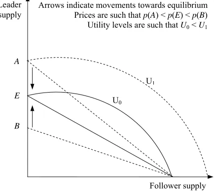
The revenues are independent of quantity. This implies that the firm’s best strategy is to set the price as high as possible. As in Grossman and Helpman (1991), the leader faces, however, an upper-bound when choosing the price that maximizes its profits. The indifference curves are concave, so consumers pur-chase only one product per variety. Firms are thus forced to engage in a Bertrand competition. For their ultimate attempt to get some market share, all firms but one set the prices just equal to the unit cost of production. The exception is the qualitative leader of each market. This firm can still set a price higher than the unit cost. This situation is illustrated in figure 2. The graph shows the qualitative leader supply on the y-axis, and the supply of the second-best product (hereafter,
the follower supply) on the x-axis. The two curves represent the indifference
curves, associated to two different levels of utility, i.e. U0<U1. The three straight lines represent the budget constraints associated to three different prices potentially set by the leader, while the follower price is just equal to the unit cost,
w. Point A corresponds to the point where the leader also sets the price equal to
the unit cost. In this case, the leader captures the entire market, and to this situa-tion is associated consumer’s maximum welfare (the supply is the same as in the case of perfect competition). The leader can profitably raise the price. The price cannot be, however, too high, e.g. as high as the price corresponding to point B,
as this would imply that the leader gives up the entire market to the follower. As-suming that consumers, when indifferent, choose the product of higher quality, the leader’s optimal choice is the price corresponding to point E.
The resulting supply function is pv(t)=cv(t)κv( )t w, where κv(t) is the
ex-ogenous rate of technological progress.22 Along with the demand function, this feature sets another difference of the present study with respect to the work of Grossman and Helpman (1991). The solution of the firm’s maximization problem
delivers a supply function, rather than a simple equilibrium price. The slope of the supply function depends on the qualitative innovation rate, and is perfectly elastic only when the latter is null. The non-innovative case reduces, in fact, to the perfect competition case, as all Bertrand games with non-differentiated agents. These features given, the role of κv(t) becomes apparent: it provides
firms with monopoly power. Firms reduce the elasticity of supply, according to the quality innovation embodied by the product. By equating the demand func-tion to the supply funcfunc-tion, we obtain the equilibrium quantity for each product, i.e.
( )
{
[
( )
]
}
( )1 1
exp v vt
v
r t t c t
w
+κ
− ρ + κ
⎧ ⎫
= ⎨ λ ⎬
⎩ ⎭
(6)
The equilibrium allocation equals that predicted by neoclassical models only Leader
supply
E
Arrows indicate movements towards equilibrium Prices are such that p(A) < p(E) < p(B) Utility levels are such that U0 < U1
U1 A
B
U0
Follower supply
if there is no innovation whatsoever up to date t. In this case, in fact,
( ) vt
κ =κv(t)=0, and cv(t)=(λw)– 1exp(r–ρ)t. When innovation is positive, we
observe two clashing effects. A positive effect is due to the average rate of inno-vation, κv
( )
t . A negative effect is due to the last rate of innovation, κv(t). Theoverall effect becomes apparent when considering the variety-specific consump-tion growth rate g[cv(t)],
23 given by
( )
[
]
( )
( )
1
v v
v
r t
g c t
t
− ρ + κ =
+ κ (7)
This growth rate is affected only by κv(t), and such influence is negative only
in case of implausibly high returns, i.e. if r>1+ρ. Suppose returns were so
re-markably high. If they reflected manufacturing productivity, production would be small.24 The supply side would deal with a market that might largely demand ne-cessities. Quality would possibly affect only prices, worsening consumer’s wel-fare. This scenario is, however, unlikely, since it would imply returns as of 100%. On the other hand, if returns are not implausibly high, quality innovation supports better economic performance. Marginal productivity is relatively low, and necessities may already be largely satiated. Increases in quality may help the economy to improve its performance, by holding the appeal of product for con-sumers at high standards. The negative effect of the last rate of innovation is suitably neutralized by its positive influence on the average rate. This is due to the great impact of the latter on consumer’s utility, as it affects a wide group of goods, i.e. all produced goods of the variety to which innovation applies.
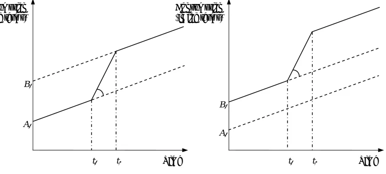
Another interesting corollary follows from the dynamics of the economy, as illustrated by figure 3. Equation (7) implies that the consumption growth rate as-sociated to the non-innovative case corresponds to the neoclassical case, formally
g[cv(t)]=r–ρ. Technical-change-augmented neoclassical models imply that two
autarkic steady-state economies, A and B, identical in all aspects but their initial
23The growth rate is computed as the difference between the logarithms of the variable at two con-secutive dates, i.e. g[y(t)]=l ny(t) – lny(t– 1). This choice implies that the growth rates suffer an infinitesimal computational error.
conditions (in figure 1, A0<B0), never converge (or diverge). This result is gen-eralized to the quality innovation case. There is, in fact, neither convergence nor divergence between economies displaying the same instantaneous rate of quality innovation. According to equation (7), qualitative differentiation may lead econ-omy A to catch up with economy B by innovating product quality, all other
con-ditions holding fixed. The opposite applies if economy B experiences an increase
in product quality innovation.
Suppose both economies have no product innovation. Their common con-sumption growth rates entirely depend on process innovation, as assumed by neoclassical models. Suppose that at some date t0, economy A begins
experienc-ing some product innovation. Economy A growth rate raises. In part (a) of figure
3, this feature is illustrated by the increase, of α degrees, of the slope of the line concerning the economy A consumption path. If product innovation lasts long
enough, economy A is able to catch up with (and perhaps overstep) economy B.
Consumption (in log terms)
Time A0
B0 α
t0 t1
Consumption (in log terms)
Time A0
B0
α
t0 t1
(a) Economy A converges towards economy B (b) Economy B diverges from economy A
The two economies follow the same consumption path if product innovation ceases right after the catching up process is completed, i.e. at date t1. On the other hand, suppose that at date t0, the economy B begins experiencing innova-tion of product quality. In part (b) of figure 3, this feature is illustrated by the
in-crease, by α degrees, of the slope of the line illustrating the consumption path of economy B. It is apparent that economy B diverges from economy A. The
expan-sion of this gap ends if product innovation ceases (or if economy A follows,
be-ginning a process of product innovation on its own, e.g. at date t1. These two ex-amples point out that this process does not revert to the initial conditions when product innovation ceases, and is due to the presence of the average rate of qual-ity innovation in the expression of the equilibrium allocation.
Equations (6) and (7) characterize the consumption bundle and its evolution. From a static perspective, variety-specific quality innovation affects quantity of each product. The consumption bundle shares thus depend on the different distri-bution of quality innovation among varieties. From a dynamic point of view, va-riety-specific quality innovation affects the consumption growth rate of each product. This implies that the consumption bundle shares are continuously changing over time. These shares clearly refer to aggregate consumption, whose growth rate is given by a weighted average of product-specific growth rates
( )
[
]
[
( )
] (
)
(
)
1 0
1 0
1 1
v v
v
g c t c t dv g C t
c t dv
− =
−
∫
∫ (8)
where C(t)≡∫10cv(t)d v defines aggregate consumption in real terms. The
weights are given by consumption of products corresponding to each variety. At early stages, quality innovation may imply that consumption of qualitatively more advanced products is smaller than less advanced products. This can be in-terpreted as follows. Since the former provide higher utility, a smaller number of units are necessary to satisfy the need at some level. As consumption increases, however, the quality spillover effect raises. As a result, consumption of
an increasing share of aggregate consumption, quality innovation plays a role of increasing importance in determining consumption aggregate growth rate.
IV. Concluding Remarks
In order to account for consumer’s statically non-homothetic preferences, this paper has introduced an objective function that accounts for quality as luxury and quantity as necessary. Using a framework similar to Grossman and Helpman (1991), and a definition of quality analogous to Stokey (1988), we have shown that such preferences generate a quality-contingent demand function. Quality is able to prevent the process, implied by neoclassical models, that leads the value of consumption to decline over time. The solution of the model implies that the equilibrium quantity is quality-contingent. Quality may also have a negative in-fluence at the early stages of economic evolution. If returns are not implausibly high, quality has a positive effect on variety-specific growth rates. Aggregate growth rate of consumption is a weighted average of variety-specific growth rates. The influence of quality on the latter passes on to the aggregate consump-tion growth rate. This is, however, positive only when the effect of quality to the static allocations of variety-specific consumption is also positive.
APPENDIX A. UTILITY FUNCTION
Consider the implicit quality-augmented utility function25
( ) ( )
[
]
{
, : c, q 0}
U= U c t q t ∈R+U U >
where c(t) and q(t) represent quality and quantity of consumption at date t
respec-tively. The utility function can be re-written as
( ) ( )
[
,]
{
[
(
( ) ( )
,)
]
: H, c, q 0}
U c t q t = u H c t q t u H H >
The inner function H(⋅) represents the flow of quality-adjusted utility that
in-dividuals derive from consumption. It can be defined as the consumption index.
In the literature, the consumption index is commonly assumed to be a homoge-neous function of c(t) and q(t). Formally, this is assured by assuming that the
ra-tio between the partial derivatives of H(⋅) to c(t) and q(t), is a homogeneous
func-tion of degree 0. It is well-known that homogeneity of H(⋅) implies homotheticity
of U(⋅), regardless of the functional form of u(⋅). In order to disregard
homo-theticity of U(⋅), therefore, the following additional assumption is required
( ) ( )
[
]
(
)
[
( ) ( )
]
( ) ( )
[
]
( ) ( )
[
]
( ) ( )
[
]
{ }
, ,
, : , \ 0,1
, ,
c c
q q
H c t q t H c t q t H c t q t
H c t q t H c t q t
+ θ θ
∈ ≠ ∀θ∈
θ θ
R R
Throughout the work presented here, we consider an explicit formulation of the individuals’ utility function, which is typically expressed by
( )
(1 ) 1( )
1 1u ⋅ = − σ ⎣− ⎡H ⋅ −σ− ⎤⎦
where H(⋅) is the consumption index, and σ represents both the risk aversion
co-efficient and the reciprocal of the consumption intertemporal elasticity of
25To simplify notation, hereafter we use
tution26. The inner function is generically expressed by a Dixit and Stiglitz (1977) type of utility function
( )
1( )
10
v v
v
H ⋅ =⎡⎣∫G ⋅η dv⎤⎦η
where Gv(⋅) represents a variety-specific quality-adjusted consumption index,
and ηv measures the degree of substitutability between variety v and all other
va-rieties. The function Gv(⋅) can be in turn expressed by
( )
( )
, 1,,
0 v s v s
t
v s v s
G ⋅ =⎡⎣∑ =B ⋅η ⎤⎦η
where Bv,s(⋅) represents a product-specific quality-adjusted consumption index,
and ηv,s measures the degree of substitutability, within variety v, between
prod-uct s and all other products. The consumption index Bv,s(⋅) is typically expressed
by
( )
( ) ( )
, , ,
v s v s v s
B ⋅ =q t c t
where qv,s(t) and cv,s(t) respectively represent quality and quantity of
consump-tion of product s and variety v. This function is homogenous in its arguments. It
follows that the instantaneous utility functions typically employed in the litera-ture are homothetic in quality and quantity of consumption. In order to get a non-homothetic instantaneous utility function, the consumption index may be ex-pressed by
( )
( )
,( ), , qv st
v s v s
B ⋅ =c t
which is non-homogeneous in its arguments. All other assumptions are standard. Varieties are independent (ηv=1–σ). The consumer is indifferent to
adjusted consumption of products of the same variety (ηv,s=1). Preferences are
homothetic, with unit consumption intertemporal elasticity of substitution (σ=1). The resulting instantaneous utility function is
( )
(
)
1{
1( )
,( ) 1}
, 0 0 1
lim 1 t qv st 1
v s s
u − =c t −σdv
σ→ ⎡ ⎤
⋅ = − σ ∫ ⎣∑ ⎦ −
The result is the indeterminate form 0/0. We can solve it by applying De l’Hôpital rule, to get
( )
1( )
,( ), 0
0ln v s
q t
t v s s
u ⋅ =∫ ⎡⎣∑ = c t ⎤⎦dv
Substituting the last equation into the objective function, we have
[ ] 1
( )
,( ),
0 0
0exp ln
v s
t q t
v s t
F=
∑
∞= −ρt ∫ ⎡⎣∫ c t ds dv⎤⎦APPENDIX B. THE CASE OF NON-UNIT INTERTEMPORAL ELASTICITY OF SUBSTITUTION
For sake of simplicity, consider the single-product case. If we abandon the as-sumption of unit intertemporal elasticity of substitution, the utility function be-comes
( )
( ) 1( )
(1 ) ( ) 11 q t
u ⋅ = − σ ⎣− ⎡c t −σ − ⎤⎦
For concavity to hold, it must be q(t)≤(1–σ)– 1. Therefore, quality is
upper-bounded. If quality increases over time, then innovation must end when
q(t)=(1–σ). If profit maximizing firms were to control quality release, this
neither theoretical nor empirical reason to be expected. Conversely, intertempo-rally non-homothetic preferences would strongly suggest that the evolution of quality perception is a stationary process. In this case, quality perception should account for some process of obsolescence.
APPENDIX C. CONSUMER’S MAXIMIZATION PROBLEM
Consider just two firms manufacturing two products of the same variety v,
and denote them by t (stands for the date t qualitative leader) and t–1 (stands for
the qualitative follower). The variety-specific consumption index is given by
( )
( )
, 1( )( )
,( ), 1 qv t t , qv tt
v v t v t
G t =c − t − +c t
Holding Gv(t)=G tv( ) fixed, we obtain the indifference curve
( )
( )
( )
, 1( ) 1,( ), , 1
qv tt v t
q t
v
v t v t
c t =⎡⎣G t −c − t − ⎤⎦
The first derivative to cv– 1(t) is given by
( )
( )
( )
( )
( )
( )( )
( ) , 1 , 1, , 1 , 1
1
, 1 , ,
0
v t
v t
q t
v t v t v t
q t
v t v t v t
c t q t c t c t q t c t
− − − − − − ∂ = − ≤ ∂
The second derivative is given by
( )
( )
[
]
( )
( )
[
( )
]
[
( )
]
( )
( )
( )
( )( )
( )[
( )
]
, 1 , 2 1, , , 1 , 1
, 1 , , 1
2
, 1 , ,
, 1
1 1 0
v t
v t
q t
v t v t v t v t
v t v t q t v t
v t v t v t
v t
c t c t q t c t
c t q t q t
c t q t c t
Since the first two derivatives are negative, the indifference curves are con-cave, and only boundary solutions apply. The individual’s dynamic maximization problem can be formalized as follows27
( ) { }
( )
( )
( ) ( )
1 0 0 1 0 0max exp( ) ln
sub exp( )
v v v t c t v v t
t q t c t dv
rt p t c t dv W
∞ =
∞ =
⎡ ⎤
−ρ ⎣ ⎦
⎡ ⎤
− ⎣ ⎦≤
∑ ∫
∑ ∫
(3)
To solve this problem, we write the following dynamic LaGrange expression
( )
[
( )
]
( ) ( )
1 1
0 0
0exp( ) v ln v 0exp( ) v v
t t q t c t dv W t rt p t c t dv
∞ ∞
= ⎡ = ⎤
=
∑
−ρ ∫ + λ⎣ −∑
− ∫ ⎦L
From the solution, we derive the set of inverse demand functions, given by
( )
( )
( )
( )
exp( ) v exp( ) 0
v
v v
q t
t rt p t
c t c t
∂ = −ρ − λ − =
∂
L
( )
[
] ( )
( )
exp ( ) v
v v q t r t p t c t − ρ =
λ (4)
where λ is a LaGrange multiplier.
APPENDIX D. PRODUCER’S MAXIMIZATION PROBLEM Recall that the variety-specific budget line is
( )
( )
( ) ( )
( )
, 1 , 1 , ,
v t v t v t v t v
p − t c − t +p t c t =E t
27We replace the notations of all variables related to product
for its ultimate attempt to get some market share, the follower chooses to set the price as pv,t– 1(t)=w, where w is the constant marginal cost. Therefore
( )
( ) ( )
( )
, 1 , ,
v t v t v t v
wc − t +p t c t =E t
As it has been shown above, only boundary solutions apply. So it can just be given by either of the following two solutions
( )
( )
( )
( )
( )
( )
( )
, 1 , , 1 ,
,
and 0; 0 and
v v
v t v t v t v t
v t
E t E t
c t c t c t c t
w p t
− = = − = =
The choice depends on the utility level assured by each candidate. Assuming that consumers purchased the product of higher quality when indifferent, the leader chooses the price that makes consumers indifferent between consuming either product. So the optimal price must be chosen according to the following equation, obtained by replacing the appropriate expenditures for consumption goods into the utility function, to get
( )
( )( )
( )
( ) , , 1 , v tv t q t
q t
v v
v t
E t E t
w p t
− ⎡ ⎤
⎡ ⎤ = ⎢
⎥
⎢ ⎥
⎣ ⎦ ⎣ ⎦
Since just one good is supplied for each variety, it must be
Ev(t)=pv,t(t)cv,t(t). Thus
( )
( )
, 1,( )( ) 1, ,
qv tt qv t t
v t v t
p t =c t − − w
Qualities qv,t(t) and qv,t– 1(t) are the first and the second best, respectively, of the need-specific market at some date t. Their ratio is given by
( )
( )
( )
[
]
( )
( )
[
( )
]
( )
, , , 1
, ,
, 1 , 1
exp
exp 1
v t v t v t
v t v t
v t v t
q t t q t
t t
q t q t
−
− −
κ
and the supply function becomes28
( )
( )
v( )tv v
p t =c t κ w
The solution of the standard profit maximization problem, given by
( )
( )
[
( )
]
( )
( )(
)
[
]
( )
( )
{
exp}
max max
v v
v v v v v
c t c t
r t
t p t w c t − ρ q t wc t
π = − = −
λ (5)
just confirm that the firm would set cv(t)=ε, where ε is a number small at
will, since cv(t) does not affect firm’s revenues. Therefore, the producer’s
opti-mal choice is the highest price that allows the firm to capture the entire market.
APPENDIX E. EQUILIBRIUM ALLOCATIONS AND GROWTH RATES
Recall that the demand and the supply functions are respectively given by
( )
[
] ( )
( )
exp ( ) v
v
v
q t r t p t
c t
− ρ =
λ
( )
( )
v( )tv v
p t =c t κ w
equating the members on the right hand side, using qv(t)=exp[κv( )t t], and
rearranging, we get the single-product equilibrium consumption allocation
( )
{
[
( )
]
}
( )1 1
exp v vt
v
r t t c t
w
+κ
− ρ + κ
⎧ ⎫
= ⎨ λ ⎬
⎩ ⎭
(6)
28Once again, we replace the notations of all variables related to product
Defining the growth rate as
( )
[
v]
ln v( )
ln v(
1)
g c t = c t − c t−
Substituting for the equilibrium allocations, we get
( )
[
]
[
( )
]
( )
(
)
[
]
(
)
(
)
ln 1 1 ln
1 1 1
v v
v
v v
r t t w r t t w
g c t
t t
− ρ + κ − λ − ρ + κ − − − λ
= −
+ κ + κ −
We have assumed that the innovation rate holds constant over time, that is
κv(t)=κv(t–1), and κv
( )
t = κ −v(
t 1)
, ∀t. Therefore, we conclude that( )
[
]
( )
( )
1 v v v r tg c t
t
− ρ + κ =
+ κ
If the average value of the innovation rate remains unchanged when the inno-vation rate holds constant, then it must be κv(t)=κv
( )
t . Therefore, we get( )
[
]
( )
( )
1 v v v r tg c t
t
− ρ + κ =
+ κ (7)
For sake of completeness, however, we need consider two other cases. The first occurs if the innovation rate is currently constant, but has changed at earlier dates, that is κv(t)=κv(t–1), and κv
( )
t ≠ κ −v(
t 1)
. The second case occurs if the innovation rate is not currently constant, that is κv(t)≠κv(t–1) and( )
(
1)
v t v t
κ ≠ κ − .
In the first case, we obtain
( )
[
]
( )
[
(
)
]
(
)
( )
1 1 1 v v pv v vr t t t t
g c t
t
− ρ + κ − κ − −
=
+ κ
( )
[
(
1)
]
(
1)
( )
v t t v t t v t
κ − κ − − = κ
substituting this value into the last equation, we get
( )
[
]
[
( )
]
( )
( )
1 pv v v v v r tg c t g c t
t
− ρ + κ
= =
+ κ
we can thus conclude that the consumption growth rate is independent of the av-erage rate of innovation, if the innovation rate stays constant during the period in which the growth rate is computed.
In the second case, we have
( )
[
]
[
( )
]
( )
(
)
[
]
(
)
(
)
ln 1 1 ln
1 1 1
v v
cv v
v v
r t t w r t t w
g c t
t t
− ρ + κ − λ − ρ + κ − − − λ
= −
+ κ + κ −
Define µ(t)=[1+κv(t)]/[1+κv(t–1)]. Multiplying and dividing by this value the second term of the right hand side, after some algebra we obtain
( )
[
]
( )
( )
( )
( )
{
[
(
)
]
(
)
}
11 1 ln
1 1
cv v
v v
v v
r t t
g c t r t t w
t t
− ρ + κ − µ
= + − ρ + κ − − − λ
+ κ + κ
Multiplying and dividing by µ(t) the second term of the right hand side, and
using the growth rate previously obtained, we get
( )
[
]
[
( )
]
( )
(
)
( )
(
)
1 ln 1 1cv v v
v v v
v
t t
g c t g c t c t
t
κ − κ −
= − −
+ κ
Given κv(t–1), the effect of an increase in κv(t) on gc v[cv(t)] is given by
( )
[
]
( )
(
)
( )
[
]
(
)
( )
[
]
(
)
2 21 1 1
ln 1
1 1
cv
v v
v
v v v
dg c t r t
c t
dk t t t
− − ρ + κ −
= − −
which is most likely negative. Therefore, an increase in the current innovation rate slackens the economy’s growth rate. This one-shot effect can be interpreted as the way individuals adapt to the new level of qualitative innovation. An in-crease in quality may lead individuals to get more satisfaction from consumption. Therefore, a smaller number of consumption units are needed to achieve a given level of utility.
Turning back to the case of constant innovation rate, we need compute the growth rate of aggregate consumption, defined by
( )
1( )
0 v
C t =∫ c t dv
to compute it, we use the following formula
( )
[
]
( )
(
)
(
)
1 1
C t C t
g C t
C t
− −
=
−
multiplying and dividing the integrand by cv(t–1), and considering that
( )
[
]
( )
(
)
(
)
1 1
v v
v
v
c t c t
g c t
c t
− −
−
we obtain
( )
[
]
[
( )
] (
)
(
)
1 0
1 0
1 1
v v
v
g c t c t dv g C t
c t dv
− =
−
∫
∫ (8)
REFERENCES
Aghion P. and Howitt P., “A Model of Growth Through Creative Destruction”,
Econometrica, 1992, 60, pp. 323-51.
Becker G. S. and Murphy K. M., “A Theory of Rational Addiction”, Journal of Political Economy, 1988, 96, pp. 675-700.
Becker G. S., Grossman M. and Murphy K. M., “Rational Addiction and the Ef-fect of Price on Consumption”, American Economic Review, 1991, 81, pp.
237-41.
Bowbrick P., The economics of quality, grades, and brands, London New York:
Routledge, 1992.
Chiang A., Fundamental Methods of Mathematical Economics, Sydney:
McGraw-Hill, 1984.
Dasgupta P. and Stiglitz J. E., “Uncertainty, Industrial Structure and the Speed of R&D”, Bell Journal of Economics, 1980, 11, pp. 1-28.
Dixit A. and Stiglitz J. E., “Monopolistic Competition and Optimum Product di-versity”, American Economic Review, 1977, 67, pp. 297-308.
Epstein L. G. and Zin S. E., “Substitution, Risk Aversion and the Temporal Be-haviour of Consumption and Attest Returns. A theoretical Framework”,
Econometrica, 1989, 57, pp. 937-69.
Grossman G. M. and Helpman E., “Quality Ladders in the Theory of Growth”,
Review of Economic Studies, 1991, 58, pp. 43-61.
Hansen G. D. and Prescott E. C., “Malthus to Solow”, American Economic Re-view, 2002, 92, pp. 1205-17.
Jones C. I., “R&D-Based Models of Economic Growth”, Journal of Political
Economy, 1995, 103, 759-84.
Judd K., “On the Performance of Patents”, Econometrica, 1985, 53, pp. 567-85.
Lancaster, K. J., “A New Approach to Consumer Theory”, Journal of Political Economy, 1966, 74, 132-57.
Eco-nomic Review, 1975, 65, 567-85.
Lancaster K. J., Variety, Equity and Efficiency, Columbia Studies in Economics, 10, New York and Guildford: Columbia University Press, 1979.
Loury G., “Market Structure and Innovation”, Quarterly Journal of Economics,
1979, 93, 395-410.
Lucas R. E. Jr., “On the Mechanics of Development Planning”, Journal of Mone-tary Economics,1988, 22, 3-42.
Romer P. M., “Endogenous Technological Change”, Journal of Political Econ-omy, 1990, 98, S71-S102.
Rosen S., “Hedonic Prices and Implicit Markets: Product Differentiation in Pure Competition”, Journal of Political Economy, 1974, 82, 34-5.
Schumpeter J.A., Capitalism, Socialism and Democracy, New York: Harper and
Brothers, 1942.
Segerstrom P. S., Anant T. C. A. and Dinopoulos E., “A Schumpeterian Model of the Product Life Cycle”, American Economic Review, 1990, 80, 1077-91.
Stokey N. L., “Learning by Doing and the Introduction of New Goods”, Journal of Political Economy, 1988, 96, 701-17.
Stokey N. L., “Human Capital, Product Quality, and Growth”, Quarterly Journal
of Economics, 1991 106, 587-616.
Xie D., “An Endogenous Growth Model with Expanding Ranges of Consumer Goods and Producers Durables”, International Economic Review, 1998, 39,
439-460.
Young A., “Learning by Doing and the Dynamic Effects of International Trade”,
Quarterly Journal of Economics, 1991, 106, 369-405.
Zweimüller J., “Schumpeterian Entrepreneurs Meet Engel’s Law: The Impact of Inequality on Innovation-Driven Growth”, Journal of Economic Growth,