Available online: https://edupediapublications.org/journals/index.php/IJR/ P a g e | 1644
Privacy Preserving Classification with Meta-learning
Prof.Dr.G.Manoj Someswar
1, K.Saisivaprasad Babu
21. Research Supervisor, Dr.APJ Abdul Kalam Technical University, Lucknow,
Uttar Pradesh, India
2. Research Scholar, Dr.APJ Abdul Kalam Technical University, Lucknow, Uttar
Pradesh, India
Abstract
This proposition is given to protection safeguarding characterization and affiliation rules mining over
unified information mutilated with randomisation-based techniques which alter singular esteems
indiscriminately to give a normal level of security. It is expected that lone contorted esteems and
parameters of a mutilating system are known amid the way toward building a classifier and mining
affiliation rules.
In this proposition, we have proposed the advancement MMASK, which wipes out exponential
multifaceted nature of assessing a unique help of a thing set as for its cardinality, and, in outcome, makes
the protection saving revelation of incessant thing sets and, by this, association rules attainable. It likewise
empowers each estimation of each credit to have diverse mutilation parameters. We indicated tentatively
that the proposed advancement expanded the precision of the outcomes for abnormal state of security. We
have likewise displayed how to utilize the randomisation for both ordinal and whole number credits to
alter their qualities as indicated by the request of conceivable estimations of these ascribes to both keep up
their unique space and acquire comparative appropriation of estimations of a property after mutilation.
Furthermore, we have proposed security saving strategies for characterization in light of Emerging
Patterns. Specifically, we have offered the excited ePPCwEP and languid lPPCwEP classifiers as security
safeguarding adjustments of enthusiastic CAEP and apathetic DeEPs classifiers, separately. We have
connected meta-figuring out how to protection safeguarding characterization. Have we utilized packing
and boosting, as well as we have joined variant likelihood circulation of estimations of properties
recreation calculations and remaking sorts for a choice tree keeping in mind the end goal to accomplish
higher exactness of order. We have demonstrated tentatively that meta-learning gives higher precision
pick up for security saving classification than for undistorted information.
The arrangements exhibited in this proposal were assessed and contrasted with the current ones. The
proposed strategies got better precision in protection saving affiliation rules mining and arrangement.
Besides, they diminished time many-sided quality of finding affiliation rules with safeguarded protection.
Available online: https://edupediapublications.org/journals/index.php/IJR/ P a g e | 1645 Introduction
On account of protection saving arrangement
with concentrated information twisted by
methods for a randomisation-based strategy
we may use no less than two calculations for
a reproduction of a probcapacity
appropriation for persistent characteristics:
AS and EM. For ostensible characteristics we
additionally have no less than two
conceivable calculations EM/AS and EQ
available to us. Consequently, we have no
less than four blends for sets containing
consistent and ostensible traits at the same
time. When we utilize a choice tree as a
classifier in protection saving, there are four
recreation sorts offered in writing, to be
specific, Local, By class, Global and Local
All.
Consolidating the presently accessible in
writing calculations for the remaking of a
probcapacity circulation and the reproduction
sorts gives no less than 16 conceivable
outcomes.[1] There is nobody mix of
calculations which performs best and we can
just pick the best blend for a particular case,
that is, for a given informational collection
and parameters of a twisting technique.
Not exclusively would we be able to call
attention to the best blend of calculations,
however it is difficult to pick the best
recreation sort. We may state that there are
two best recreation sorts: Local and By class,
however regardless we can't pick the best
remaking sort. The analyses directed in
demonstrated that these two reproduction
sorts are the best while building choice trees
over twisted information containing just
nonstop traits. affirmed this announcement
for nonstop and ostensible properties utilized
at the same time. The two papers did not call
attention to the best reproduction sort in light
of the fact that for a few informational
collections Local gives better outcomes, for
others By class.
Considering the high number of blends of
calculations and remaking sorts, we propose
to utilize meta-learning to dispense with
these downsides. In security preserving
information mining we may utilize
meta-learning (without various leveled structures)
in two situations. The primary situation is to
apply stowing or boosting for a picked blend
of calculations and a remaking sort. In the
second situation, sacking or boosting
techniques are connected independently to
each unique blend of calculations and
recreation sorts. Therefore, extraordinary
base classifiers are utilized, as opposed to the
primary approach where just a single base
classifier is considered. In the two situations
we utilize all classifiers together and
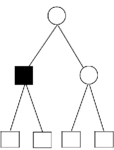
Available online: https://edupediapublications.org/journals/index.php/IJR/ P a g e | 1646 Figure 1: The decision tree and the probabilities for tests
Boosting for Distorted Data
It is accepted that a classifier is prepared over
contorted information, however test over
undistorted information. Boosting needs to
arrange prepare (misshaped) information to
register probabilities Pil and I portions.
Ordering misshaped information in an
indistinguishable way from we arrange
undistorted information prompts mistake. In
this segment, we propose how to characterize
prepare (contorted) information to have the
capacity to utilize boosting for misshaped
information.[2]
In a standard test hub in a (parallel) choice
tree, a given estimation of a trait is checked
whether it meets a test condition or not. Give
us a chance to expect that the left branch is
picked when it meets a test and the correct
branch when it doesn't. Having a contorted
esteem xA of a property A, we may figure
the likelihood PA(yes) that a given esteem
xA meets a test condition and the likelihood
PA(no) that it doesn't meet a test condition,
PA(no) = 1 PA(yes).
For a specimen S that we need to order we
figure the likelihood P li for I-th leaf that the
example S could fall into this leaf. This
likelihood is equivalent to the augmentation
of probabilities PX (yes) when we pick a left
branch and PX (no) when we pick a correct
branch for each test in the way which
prompts I-th leaf.
Give us a chance to expect there is a choice
tree with 3 tests, that is, inner hubs (see
Figure 1): the principal test on a quality An
in the root, second on a trait B on the left,
and third on a characteristic C on the right.
The likelihood of the leaf l1 is P l1 = PA(yes)
PB(yes).
Having evaluated the probabilities for l
leaves, we can compute the likelihood that
the specimen S has a place with the
Available online: https://edupediapublications.org/journals/index.php/IJR/ P a g e | 1647 i2faj X a jg
PS(Cj) = P li
LeafCategory =C
We choose the category with the highest
probability and assign it to the sample S.To
calculate PS(Cj), we need to estimate PX (yes)
and PX (no) for each test. We propose the
solution for nominal and continuous
attributes in the subsequent sections.
Calculating Probabilities for Nominal
Tests
For nominal attributes we calculate the
probability PX (yes), the probability PX (no)
can be calculated as PX (no) = 1 PX (yes), in
the following way:
Let us assume that X is an original nominal
attribute and Z is a modified attribute. For an
internal node m we know modified values
(all train samples which go into this node) of
a nominal attribute, so we can determine a
probability distribution (i.e., P (Z = vi); i = 1;
:::; k) of the modified attribute Z. Having
modified values of the attribute Z, we can
perform the reconstruction using either the
EM/AS or EQ algorithm and obtain the
reconstructed probability distribution (P (X =
vi); i = 1; :::; k).
Let us assume that the distorted value of the attribute Z is equal to vq (Z = vq). We can calculate probabilities that
P (X = vijZ = vq); i = 1; :::; k. Using Bayes’ Theorem, we obtain:
P(X=vijZ=vq) =P(X=vi) P (Z = vqjX=vi):
P (Z = vq)
P (Z = vqjX = vi) is the probability that the value vi of the attribute X will be changed to the value vq and that
probability is known because parameters of the distorting method are given. In order to calculate PX (yes), we
sum probabilities P (X = vijZ = vq) for all values vi
which meet a test condition.
2f jX
PX (yes) = P (X = vijZ = vq)
i a va2testg
Calculating Probabilities for Continuous Tests
For continuous attributes and the additive
perturbation we calculate the probability PX
(yes) in the following way: Let X be an
original attribute. Y is used to modify X by
means of the additive perturbation and obtain
an attribute Z. Let Z be equal to z. Let us
assume that a continuous test is met if the
value of the attribute X is less than or equal
Available online: https://edupediapublications.org/journals/index.php/IJR/ P a g e | 1648 PX (yes) = P (X tjZ = z; X + Y = Z) = F (tjZ = z; X + Y = Z):
PX (yes) =
Z t
fX (rjZ = z; X + Y = Z)dr:
1
Using Bayes’ Theorem, we obtain:
t f Z z; X Y = Z X = r)f (r)
PX (yes) = Z 1
Z ( =
+j
X
dr:
fZ (z)
Since Y is independent of X and the denominator is independent of the integral, then:
P (yes) = T
fY (z r)fX (r) dr:
X Z 1 fZ (z)
fY is known, hence we can compute PX (yes) and PX (no).
For the retention replacement perturbation we calculate PX (yes) probability in the following way: Let X be an
original attribute and Z be a modified attribute obtained from X by means of the retention replacement
perturbation. Let Z be equal to z. Let us assume that a continuous
test is met if the value of the attribute X is less than or equal to t. Then, we may write:
PX (yes) = P (X tjZ = z):
Let 1(condition) be an indicator function which takes 1 when condition is met and 0 oth-erwise.
T
PX (yes) =p1(z < t) + (1 p)Z
dming(rjX)dr;
where g() is a density function of a distorting distribution used in the retention replacement perturbation.
Since g() is independent of X, we obtain:
X (yes) = p 1(z < t) + (1 p) Z
T
dmin g(r)dr:
Assuming a uniform distribution as the distorting distribution for the retention replacement perturbation, we can
write:
P
X
(yes) = p 1(z < t) + (1 p) t dmin ;
dmax dmin
Available online: https://edupediapublications.org/journals/index.php/IJR/ P a g e | 1649 Bagging and Boosting for Chosen
Combination of Algorithms and
Reconstruction Type
Having picked a mix of calculations for a
remaking of a likelihood conveyance, one
calculation for consistent qualities and
second calculation for ostensible
characteristics, and a reproduction sort to be
utilized as a part of a choice tree, we may
utilize packing or boosting. A last class is
resolved by a basic or weighted voting
technique.
We may likewise join votes from sacking and
boosting at one time and ascertain the last
class. In our approach votes are consolidated
at a similar level, that is, progressive
classifiers are not utilized. For this situation,
we pick various classifiers for each
meta-learning technique independently.[3] For
stowing weights are equivalent to 1 and for
boosting we utilize I portion as weights. For
instance, let us expect that a choice class is a
paired (0-1) quality, the quantity of
classifiers for sacking is 3 and for boosting is
4. For an example S we total weights for all
classifiers which addressed 0 and for all
classifiers which addressed 1.Having chosen
a combination of algorithms for a
reconstruction of a probability distribution,
one algorithm for continuous attributes and
second algorithm for nominal attributes, and
a reconstruction type to be used in a decision
tree, we may use bagging or boosting. A final
class is determined according to a simple or
weighted voting method.
We may also join votes from bagging and
boosting at one time and calculate the final
class. In our approach votes are combined at
the same level, that is, hierarchical classifiers
are not used. In this case, we choose a
number of classifiers for each meta-learning
method separately. For bagging weights are
equal to 1 and for boosting we use i fraction
as weights.
For example, let us assume that a decision
class is a binary (0-1) attribute, the number of
classifiers for bagging is 3 and for boosting is
4. For a sample S we sum weights for all
classifiers which answered 0 and for all
classifiers which answered 1.
j=1::7X
j(S)=0 Xj(S)=1
W0 = wj; W1 = wj
;cl j=1::7;cl
Then we choose a class with the highest sum (cumulative weight)
Combining Different Algorithms and
Reconstruction Types with
Usage of Bagging and Boosting
There are three conceivable instances of
utilizing distinctive calculations and
reproduction sorts with meta-learning. We
may utilize distinctive mixes of calculations
or diverse recreation sorts. For every blend of
reproduction calculations and a picked
Available online: https://edupediapublications.org/journals/index.php/IJR/ P a g e | 1650 either sacking or boosting, as in this research
paper. At that point we decide a last class
utilizing all made classifiers by (weighted)
voting (all classifiers are on a similar level
and we total all weights). For various
recreation sorts and
a picked mix of calculations we process
similarly concerning the case with various
calculations, that is, for every remaking sorts
and a picked mix of calculations we utilize
either stowing or boosting and afterward we
decide a last class utilizing all made
classifiers by voting.[4]
We may likewise consolidate these
circumstances, that is, we utilize sacking or
boosting for every conceivable mix of
calculations and remaking sorts. The strategy
for ascertaining weights continues as before.
In all cases we may incorporate not every
single conceivable blend to accomplish better
exactness of characterization, e.g., just Local
and By class for various mixes of
reproduction sorts.
Exploratory Evaluation
This segment displays the consequences of
the tests directed with the utilization of
meta-learning in protection safeguarding
arrangement. All sets utilized as a part of
tests can be downloaded from UCI Machine
Learning Repository. We utilized the
accompanying sets: Australian,
Credit-g,Diabetes, Segment, picked under the
accompanying conditions: two sets ought to
contain just consistent characteristics
(Diabetes, Segment), two different sets both
constant and ostensible properties
(Australian, Credit-g), one of the sets ought
to have a class property with numerous
esteems (Segment).[5]
In the trials the exactness, affectability,
specificity, accuracy and F-measure were
utilized. We utilized likewise the meaning of
protection in view of the differential entropy.
To accomplish more solid outcomes, we
utilized 10-overlay cross-approval and
ascertained the normal of 50 numerous runs.
In all trials we mutilated all qualities with the
exception of class/target trait. Every single
consistent property were mutilated by
methods for the added substance annoyance
with a uniform dispersion, unless expressly
expressed that either a typical appropriation
or the maintenance supplanting bother with a
uniform dissemination was utilized. We
utilized the SPRINT choice tree changed to
fuse security as indicated in is research
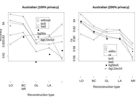
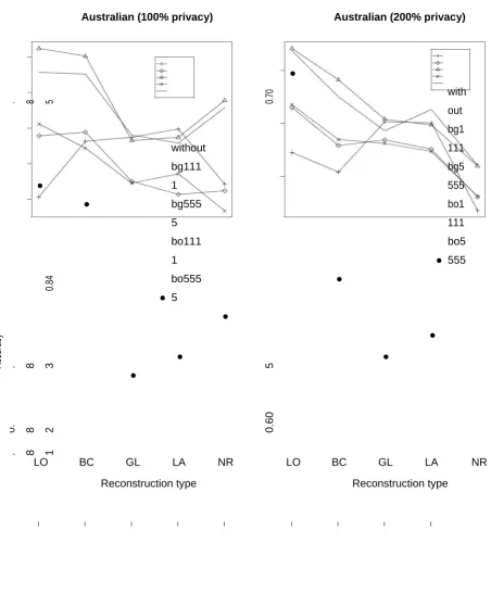
Available online: https://edupediapublications.org/journals/index.php/IJR/ P a g e | 1651 Figure 2: The accuracy of classification with the usage of meta-learning (bagging and boosting
methods) for the set Australian with 100% and 200% privacy level for the chosen combination
of algorithms - AS.EA
Australian (100% privacy) Australian (200% privacy)
0. 84
Acc
u
rac
y
0.83
0.82
0.8
1
without bo5
● ba5
●
● bg5bo 5
bg11bo10
● ●
●
LO BC GL LA
NR
Reconstruction type
0. 64
0.62
Acc
u
ra
cy 0.60
0.5
8
0.56
●
●
● ●
witho ut
●
bo5 ba5 ● bg5bo5
bg11bo10
LO BC GL LA NR
Available online: https://edupediapublications.org/journals/index.php/IJR/ P a g e | 1652
Experiments with Chosen
Combination of Algorithms and
Reconstruction Type with Usage of
Bagging and Boosting
Figure 2 demonstrates the precision of
arrangement for Australian set. We utilized
the accompanying mix of calculations:
AS.EA, i.e., AS for nonstop characteristics
and EM/AS (called EA) for ostensible
qualities and directed tests for every
conceivable sort of recreation:[6] LO, Local;
BC, By class; GL, Global; LA, Local all. NR
implies that we didn't utilize any
reconstruction. We utilized packing and
boosting independently and consolidated, as
depicted in this research paper. We
additionally tried different things with the
quantity of classifiers for a given
meta-learning strategy. Figure 2 presents the
outcomes for the different use of sacking -
bg5 (5 classifiers were utilized), boosting bo5
(with 5 classifiers) and the mix of
meta-learning strategies, e.g., bg5bo4 - stowing
utilized 5 classifiers and boosting 4 choice
trees (the number after short name of a
meta-learning technique signifies what number of
classifiers were utilized for a specific
meta-learning strategy).[10] Without implies that
no meta-learning strategy was utilized, i.e., a
solitary classifier was assembled. For Local
and By class recreation sorts and both
exhibited levels of protection (100%, 200%)
we got for each situation higher precision.
For 100% level of protection precision was
around 84-85%. 200% level of security
lessens precision to the level of 62-64%.[7]
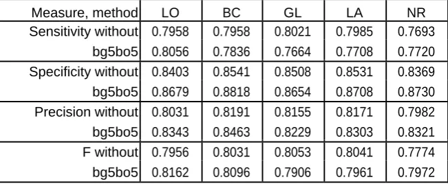
Table 1: The sensitivity, specificity, precision and F-measure with the usage of meta-learning
(bagging and boosting methods) for the set Australian with 100% privacy level for the chosen
combination of algorithms - AS.EA
Measure, method LO BC GL LA NR
Sensitivity without 0.7958 0.7958 0.8021 0.7985 0.7693
bg5bo5 0.8056 0.7836 0.7664 0.7708 0.7720
Specificity without 0.8403 0.8541 0.8508 0.8531 0.8369
bg5bo5 0.8679 0.8818 0.8654 0.8708 0.8730
Precision without 0.8031 0.8191 0.8155 0.8171 0.7982
bg5bo5 0.8343 0.8463 0.8229 0.8303 0.8321
F without 0.7956 0.8031 0.8053 0.8041 0.7774
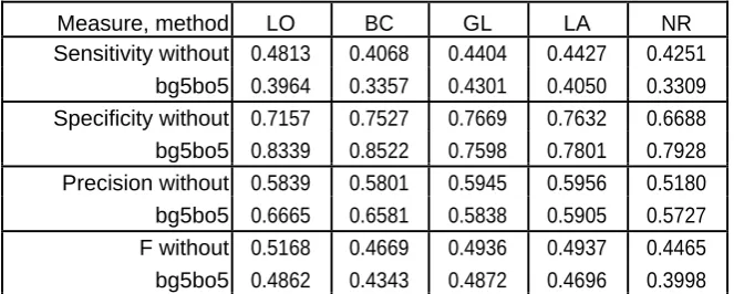
Available online: https://edupediapublications.org/journals/index.php/IJR/ P a g e | 1653 (bagging and boosting methods) for the set Australian with 200% privacy level for the chosen
combination of algorithms - AS.EA
Measure, method LO BC GL LA NR
Sensitivity without 0.4813 0.4068 0.4404 0.4427 0.4251
bg5bo5 0.3964 0.3357 0.4301 0.4050 0.3309
Specificity without 0.7157 0.7527 0.7669 0.7632 0.6688
bg5bo5 0.8339 0.8522 0.7598 0.7801 0.7928
Precision without 0.5839 0.5801 0.5945 0.5956 0.5180
bg5bo5 0.6665 0.6581 0.5838 0.5905 0.5727
F without 0.5168 0.4669 0.4936 0.4937 0.4465
bg5bo5 0.4862 0.4343 0.4872 0.4696 0.3998
For 100% level of privacy bagging with 5
classifiers achieved better results than
bagging and boosting together both with 5
classifiers. However, for 200% level of
privacy bagging and boosting together with 5
classifiers per each method performed better.
For Global and Local all meta-learning
decreased the accuracy of classification. The
reason may be that in these two
reconstruction types we do not divide
samples into classes during the
reconstruction and changes made for each
training set have low influence on a decision
of classifiers. For 100% level of privacy
without reconstruction meta-learning
increased accuracy. We may say that it was
as high as for Global and Local all. For 200%
level of privacy and without the
reconstruction meta-learning still yielded
better results, but the overall accuracy was
the lowest compared to the accuracy of all
reconstruction types. Tables 1 and 2 show the
sensitivity, specificity, precision and
F-measure for the set Australian in this
experiment. For 100% level of privacy with
Local and By class reconstruction types only
the sensitivity for By class has lower value
for meta-learning with the simultaneous use
of stowing and boosting with 5 classifiers for
every technique, contrasted with the case
without meta-learning. For 200% level of
security with Local and By class we got
bring down qualities for the affectability and
Available online: https://edupediapublications.org/journals/index.php/IJR/ P a g e | 1654 Figure 3: The accuracy of classification with the usage of meta-learning (bagging and boosting
methods) for the set Australian with 100% and 200% privacy level for the different
combinations of algorithms and the chosen reconstruction type
Australian (100% privacy) Australian (200% privacy)
0 . 8 5 0.70
●
with
out
without
bg1
111
●
●
bg111
1
bg5
555
bg555
5
bo1
111
0.8
4
bo111
1 ●
bo5
555
● bo555
5
●
●
●
Ac
cu
ra
cy
A c c u r a c y
0 . 8 3 ● 0.6 5 ●
●
0. 8 2 0.60
0 . 8 1
LO BC GL LA NR LO BC GL LA NR
Available online: https://edupediapublications.org/journals/index.php/IJR/ P a g e | 1655 somewhat bring down extent of genuine
positives which were effectively
distinguished all things considered.[11] For
200% level of protection with Global and
Local all recreation sorts meta-learning
yielded better outcomes just in two cases: the
affectability for Global and the specificity for
Local all. For 100% level of protection all
measures were between around 77% and
86%, for 200% the affectability diminished
to the level of 33%. To whole up, we can
state that all in all the higher number of
classifiers is utilized, the better precision
meta-learning yields. The concurrent
utilization of two meta-learning strategies
with high number of classifiers yields comes
meta-learning strategy.
Precision of Classification for
Different Combinations of Algorithms
with Usage of Bagging and Boosting
We played out the tests with the utilization of
all blends of calculations: AS.EA, EM.EA,
AS.EQ, and EM.EQ (Figure 3). We utilized
independently sacking and boosting with 1
and 5 classifiers for each every mix of
reproduction calculations and a picked
recreation sort (bg1111 indicates stowing
with 1 classifier for each every mix of
remaking calculations, bo5555 implies
boosting with 5 classifiers for each every
blend of calculations, and so forth.).
Australian set
8 5 0 .
●
8 0 0 .
●
Acc
u
ra
cy
● ●
7 0 7 5 0 . 0 . m100%
m150%
m200%
Lo100%
● Lo150%
Lo200%
6 5 0 .
6 0 0 .
AS.EA EM.EA AS.EQ
EM. EQ
Algorithms
Figure 4: The accuracy of classification with the usage of meta-learning (simultaneously bagging
and boosting with 5 classifiers per each method) for the set Australian with 100%, 150%, and
200% privacy level for only Local and By class reconstruction types compared to Local
Available online: https://edupediapublications.org/journals/index.php/IJR/ P a g e | 1656 The obtained results were similar to those
from the experiment presented in this
research paper. Meta-learning yielded better
results for Local, By class and no
reconstruction, but almost no improvement
for Global and Local all. For 5 classifiers per
combination of algorithms (for Local and By
class) we obtained high accuracy, about 85%
for 100% level of privacy and about 72% for
200% level of privacy. For bagging and
boosting with 1 classifier per each
combination of algorithms we observed
lower accuracy, but still higher than without
meta-learning (except for one case). To
conclude, by using different combinations of
algorithms, we obtained high accuracy. The
higher number of classifiers was used, the
better results meta-learning yielded. Global
and Local all reconstruction types yielded
poor results for meta-learning.
Ac curacy of Classification for Different
Reconstruction Types with Usage of
Meta-learning
For the set Australian with the usage of
meta-learning for all combinations of
reconstruction types we obtained worse
results than without meta-learning because
we obtained really low accuracy for Global
and Local all reconstruction types for the set
Australian and the results of the previous
experiments in this chapter confirmed that
these two reconstruction types seem to be the
worst and for some sets they yield very poor
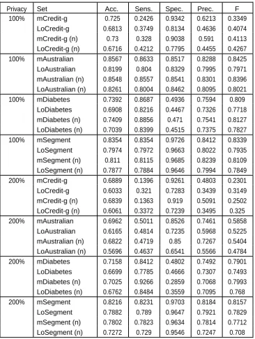
Available online: https://edupediapublications.org/journals/index.php/IJR/ P a g e | 1657 Table 3: The accuracy of classification with the usage of meta-learning (simultaneously bagging
and boosting with 5 classifiers per each method) for only Local and By class reconstruction
types and different combinations of algorithms compared to Local reconstruction type and
AS.EA algorithms
Privacy Set Acc. Sens. Spec. Prec. F
100% mCredit-g 0.725 0.2426 0.9342 0.6213 0.3349
LoCredit-g 0.6813 0.3749 0.8134 0.4636 0.4074
mCredit-g (n) 0.73 0.328 0.9038 0.591 0.4113
LoCredit-g (n) 0.6716 0.4212 0.7795 0.4455 0.4267
100% mAustralian 0.8567 0.8633 0.8517 0.8288 0.8425
LoAustralian 0.8199 0.804 0.8329 0.7995 0.7971
mAustralian (n) 0.8548 0.8557 0.8541 0.8301 0.8396
LoAustralian (n) 0.8261 0.8004 0.8462 0.8095 0.8021
100% mDiabetes 0.7392 0.8687 0.4936 0.7594 0.809
LoDiabetes 0.6908 0.8216 0.4467 0.7326 0.7718
mDiabetes (n) 0.7409 0.8856 0.471 0.7541 0.8127
LoDiabetes (n) 0.7039 0.8399 0.4515 0.7375 0.7827
100% mSegment 0.8354 0.8354 0.9726 0.8412 0.8339
LoSegment 0.7974 0.7972 0.9663 0.8022 0.7935
mSegment (n) 0.811 0.8115 0.9685 0.8239 0.8109
LoSegment (n) 0.7877 0.7884 0.9646 0.7994 0.7849
200% mCredit-g 0.6889 0.1396 0.9261 0.4803 0.2301
LoCredit-g 0.6033 0.321 0.7283 0.3439 0.3149
mCredit-g (n) 0.6839 0.1363 0.919 0.5091 0.2502
LoCredit-g (n) 0.6061 0.3372 0.7239 0.3495 0.325
200% mAustralian 0.6962 0.5011 0.8526 0.7461 0.5858
LoAustralian 0.6165 0.4814 0.7235 0.5968 0.5225
mAustralian (n) 0.6822 0.4719 0.85 0.7267 0.5404
LoAustralian (n) 0.5696 0.4637 0.6541 0.5566 0.4784
200% mDiabetes 0.7158 0.8412 0.4802 0.7492 0.7901
LoDiabetes 0.6699 0.7785 0.4666 0.7307 0.7493
mDiabetes (n) 0.7025 0.9266 0.2859 0.7068 0.7993
LoDiabetes (n) 0.6762 0.8484 0.3559 0.7095 0.768
200% mSegment 0.8216 0.8231 0.9703 0.8184 0.8157
LoSegment 0.7882 0.789 0.9647 0.7921 0.7829
mSegment (n) 0.7802 0.7823 0.9634 0.7814 0.7712
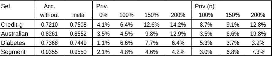
Available online: https://edupediapublications.org/journals/index.php/IJR/ P a g e | 1658 Table 4: The comparison of the meta-learning accuracy gain for undistorted and distorted data
(the simultaneous usage of bagging and boosting with 5 classifiers per each method)
Set Acc. Priv. Priv.(n)
without meta 0% 100% 150% 200% 100% 150% 200%
Credit-g 0.7210 0.7508 4.1% 6.4% 12.6% 14.2% 8.7% 9.1% 12.8%
Australian 0.8261 0.8552 3.5% 4.5% 9.8% 12.9% 3.5% 6.6% 19.8%
Diabetes 0.7368 0.7449 1.1% 6.6% 7.7% 6.4% 5.3% 3.7% 3.9%
Segment 0.9355 0.9550 2.1% 4.8% 4.6% 4.2% 3.0% 6.8% 7.3%
To dispose of the bothersome effect of
Global and Local all, we utilized just Local
and By class reproduction sorts. The after
effects of the tests for the set Australian are
appeared in Figure 4. Just for two best
recreation sorts meta-learning performed
superior to a solitary classifier. For 100%
level of protection the exactness was around
85%, for 150% marginally bring down -
82-83%. For 200% level of security we got 65%
of the exactness for AS.EA and EM.EA,
calculations AS.EQ and EM.EQ yielded
precision around 72%.
Precision of Classification for
Different Combination of Algorithms
and Reconstruction Types with Usage
of Bagging and Boosting
The last plausibility is to consolidate
distinctive calculations and remaking sorts.
As indicated by the outcomes from the past
segment we utilize just Local and By class
sorts of remaking.[12]
The after effects of the trials are appeared in
Table 3. The sets utilized as a part of these
experiments were twisted by methods for the
added substance bother with either a uniform
or typical dispersion (mCredit-g implies that
the set Credit-g was contorted with a uniform
circulation and meta-learning was utilized,
LoCredit-g illuminates that Local
reproduction sort and AS.EA calculations
were utilized, mCredit-g (n) implies that the
set was mutilated by methods for an ordinary
appropriation, and so forth.). Just for Credit-g
meta-adapting fundamentally diminished the
affectability and F-measure. In the rest of the
cases, meta-learning yielded higher measures
(there was just a single case with the
altogether more awful outcome, the
specificity for Diabetes set, 200% level of
security and an ostensible contortion
dissemination).
Table 4 demonstrates the precision (indicated
as Acc.) without (signified as without) and
with (meant as meta) meta-learning without
protected security and the relative pick up
caused by meta-learning for undistorted
information (Priv. 0%) and security
safeguarded information for a uniform
contorting dispersion (Priv. 100%-200%) and
an ordinary (Priv.(n) 100%-200%) contorting
conveyances. In all cases meta-learning pick
up for level of protection 100%, 150%, and
200% was higher than for undistorted
information.
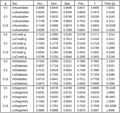
Table 5 presents the after effects of the try
different things with joining distinctive
Available online: https://edupediapublications.org/journals/index.php/IJR/ P a g e | 1659 methods for the maintenance supplanting
bother with a uniform circulation and p 2
f0:5; 0:3; 0:15g (mCredit-g implies that
meta-learning was utilized for the set
Credit-g, LoCredit-g educates that Lo-cal
reproduction sort and AS.EA calculations
were utilized, and so forth.). After bending,
constant at-tributes were discretised into 5
containers each of which secured level with
number of samples1. Correspondingly
1 The outcomes for discretisation into 10
containers can be found in Appendix A.3. to
perturbation, meta-learning significantly
decreased the sensitivity and F-measure only
for Credit-g. In the remaining cases,
meta-learning yielded higher measures (there were
only two cases with the significantly worse
results, the specificity for Diabetes set and p
2 f0:3; 0:15g).
In the presented experiments, application of
meta-learning increased accuracy once again
proving its usefulness in privacy preserving
data mining.[13]
Table 5: The accuracy of classification with the usage of meta-learning (simultaneously bagging
and boosting with 5 classifiers per each method) for only Local and By class reconstruction
types and dif-ferent combinations of algorithms compared to Local reconstruction type and
AS.EA algorithms and the retention replacement perturbation
p Set Acc. Sens. Spec. Prec. F Time [s]
0.5 mAustralian 0.8586 0.8444 0.8698 0.8427 0.8406 7.9231
LoAustralian 0.8203 0.8012 0.8358 0.8004 0.7975 0.1108
0.3 mAustralian 0.8443 0.8033 0.8766 0.8433 0.8184 8.1545
LoAustralian 0.7748 0.7430 0.8003 0.7531 0.7436 0.1212
0.15 mAustralian 0.7449 0.5885 0.8676 0.7861 0.6653 10.8198
LoAustralian 0.6300 0.5275 0.7099 0.6001 0.5539 0.2533
0.5 mCredit-g 0.7232 0.2890 0.9105 0.5793 0.3771 7.3214
LoCredit-g 0.6688 0.4080 0.7813 0.4443 0.4192 0.1411
0.3 mCredit-g 0.7030 0.1779 0.9295 0.5240 0.2716 7.0203
LoCredit-g 0.6360 0.3844 0.7441 0.3934 0.3788 0.1688
0.15 mCredit-g 0.6834 0.1354 0.9188 0.4431 0.2601 8.1628
LoCredit-g 0.5799 0.3783 0.6669 0.3285 0.3403 0.2246
0.5 mDiabetes 0.7302 0.8366 0.5311 0.7665 0.7982 2.1204
LoDiabetes 0.6837 0.7718 0.5212 0.7488 0.7570 0.0221
0.3 mDiabetes 0.7115 0.8429 0.4654 0.7448 0.7886 2.1381
LoDiabetes 0.6436 0.7345 0.4729 0.7209 0.7243 0.0286
0.15 mDiabetes 0.6710 0.8641 0.3164 0.7011 0.7708 2.2153
LoDiabetes 0.5974 0.7058 0.4001 0.6859 0.6909 0.0380
0.5 mSegment 0.8730 0.8728 0.9788 0.8760 0.8695 78.1030
LoSegment 0.8291 0.8293 0.9715 0.8318 0.8239 1.0958
0.3 mSegment 0.8183 0.8182 0.9697 0.8261 0.8120 85.9497
LoSegment 0.7382 0.7387 0.9564 0.7418 0.7249 1.3034
0.15 mSegment 0.7252 0.7252 0.9542 0.7310 0.7058 101.6288
Available online: https://edupediapublications.org/journals/index.php/IJR/ P a g e | 1660 Time of Training Classifiers with
Meta-learning
Sadly, meta-learning expands time of
preparing on the grounds that few classifiers,
e.g., decision trees, should be assembled,
which requires some serious energy.
Considering time of preparing for various
remaking sorts for a choice tree, Local is the
most costly on the grounds that it reproduces
a likelihood appropriation for each class in
each hub of a choice tree. By class sets aside
just somewhat more opportunity (for high
number of classifiers) than the case without
the remaking, since it plays out the recreation
for each class, however just in a base of a
tree.[11] For around 20 classifiers there is a
distinction in time of preparing of one
request of extent contrasted with the case
without meta-learning. Contrasting
additionally the outcomes introduced in
Table 5, where 80 classifiers were utilized,
the distinction in compressed time of
preparing and arrangement is in the vicinity
of one and two requests of greatness
contrasted with the case with one classifier.
Meta-learning expands time of preparing, yet
the season of characterization is still little
and practically the same. Meta-learning is an
ideal way to deal with utilize disseminated
calculations and prepare classifiers on
various machines.[14] This would diminish
time expected to prepare classifiers.
Conclusions and Future Work
In protection safeguarding information
digging for order meta-learning can be
utilized to accomplish the higher precision
and consolidate data from various
calculations. The led tests demonstrated that
it is smarter to consolidate just Local and By
class recreation sorts than all the remaking
sorts in light of the fact that Global and
Local All may yield poor outcomes (likely
because of the reproduction performed for
information not separated into classes).
Meta-learning gives higher pick up in
precision for information with safeguarded
security than for undistorted information
since joins extra data from various likelihood
remaking calculations and sorts of recreation
contrasted with the case without protection,
where probability reproduction calculations
are not utilized. Also, meta-learning
enhances comes about when
"temperamental" learning calculations are
utilized and classifiers with various
likelihood reconstruction calculations and
recreation sorts might be viewed in that
capacity since they yield essentially unique
outcomes for various remaking calculations
and reproduction sorts. Lamentably,
meta-learning expands time of preparing
classifiers. Time of grouping is still
altogether littler than time of preparing
classifiers. Moreover, meta-learning makes
harder an understanding of a made classifier.
One needs to take a gander at all choice trees
to know principles of characterization. Later
on, we intend to examine the likelihood of
expansion of our outcomes to the utilization
of different grouping calculations as
meta-students (not just straightforward or
weighted voting).[15] We will check comes
about for the situation where each and every
execution of packing and boosting yields
independently its own response to a classifier
of the more elevated amount (in opposition
to the case exhibited in this proposal). It is
likewise conceivable to go to a classifier of
the more elevated amount answers of
classifiers, as well as the preparation set or
its subset. We additionally plan to utilize
Available online: https://edupediapublications.org/journals/index.php/IJR/ P a g e | 1661 classifiers with, e.g., distinctive mixes of
calculations and a similar recreation sort, and
after that prepare a classifier on the most
elevated amount on their yields. We might
want to utilize the introduced way to deal
with arrange a contorted test set. To diminish
time of Ashok Savasere, Edward
Omiecinski, and Shamkant B. Navathe. An
efficient algorithm for mining association
rules in large databases.
1. In Dayal et al., pages 432–444. Yücel
Saygin, Vassilios S. Verykios, and Chris
Clifton. Using unknowns to prevent
discovery of association rules. SIGMOD
Record, 30(4):45–54, 2001.
2. Yücel Saygin, Vassilios S. Verykios, and
Ahmed K. Elmagarmid. Privacy preserving
association rule mining. In RIDE, pages
151–158, 2002.
3. John C. Shafer, Rakesh Agrawal, and
Manish Mehta. Sprint: A scalable parallel
classifier for data mining. In C. Mohan
Nandlal L. Sarda T. M. Vijayaraman,
Alejandro P. Buch-mann, editor, VLDB’96,
Proceedings of 22th International Conference
on Very Large Data Bases, September 3-6,
1996, Mumbai (Bombay), India, pages 544–
555. Morgan Kaufmann, 1996.
4. Mark Shaneck, Yongdae Kim, and Vipin
Kumar. Privacy preserving nearest neighbor
search. In ICDM Workshops, pages 541–
545. IEEE Computer Society, 2006.
5. Mark Shaneck, Yongdae Kim, and Vipin
Kumar. Privacy preserving nearest neighbor
University of Minnesota, 2006.
6. Claude E. Shannon. A mathematical
theory of communication. Bell system
technical journal, 27, 1948.
7. Ramakrishnan Srikant and Rakesh
Agrawal. Mining generalized association
rules. In Dayal et al. [35], pages 407–419.
8. Ramakrishnan Srikant and Rakesh
Agrawal. Mining quantitative association
rules in large relational tables. In H. V.
Jagadish and Inderpal Singh Mumick,
editors, SIGMOD Conference, pages 1–12.
ACM Press, 1996.
9. Lambert M. Surhone, Miriam T.
Timpledon, and Susan F. Marseken. Pearson’s Chi-Square Test. Betascript
Publishers, Beau Bassin, 2010.
10. Alan Taylor and William Zwicker. A
characterization of weighted voting. In Proc.
of the AMS, pages 1089–1094, 1992.
11. Li-Min Tsai, Shu-Jing Lin, and Don-Lin
Yang. Efficient mining of generalized
nega-tive association rules. In Xiaohua Hu, Tsau
Young Lin, Vijay V. Raghavan, Jerzy W.
Grzymala-Busse, Qing Liu, and Andrei Z.
Broder, editors, GrC, pages 471–476. IEEE
Computer Society, 2010.
12. Jaideep Vaidya and Chris Clifton.
Privacy preserving association rule mining in
vertically partitioned data. In KDD, pages
639–644. ACM, 2002.
13. Jaideep Vaidya and Chris Clifton.
Privacy preserving naïve Bayes classifier for
Available online: https://edupediapublications.org/journals/index.php/IJR/ P a g e | 1662 14. Jaideep Vaidya and Chris Clifton.
Privacy-preserving decision trees over
vertically par-titioned data. In DBSec, pages
139–152, 2005.
15. Jaideep Vaidya, Chris Clifton, Murat
Kantarcioglu, and A. Scott Patterson.
Privacy-preserving decision trees over
vertically partitioned data. TKDD, 2(3),
2008.
preparing classifiers in meta-learning, we