DOI: 10.1534/genetics.105.046417
High-Resolution Association Mapping of Quantitative Trait Loci:
A Population-Based Approach
Ruzong Fan,*
,1Jeesun Jung
†and Lei Jin*
*Department of Statistics, Texas A&M University, College Station, Texas 77843 and†Department of Human Genetics, University of Pittsburgh, Graduate School of Public Health, Pittsburgh, Pennsylvania 15261
Manuscript received June 2, 2005 Accepted for publication September 19, 2005
ABSTRACT
In this article, population-based regression models are proposed for high-resolution linkage disequi-librium mapping of quantitative trait loci (QTL). Two regression models, the ‘‘genotype effect model’’ and the ‘‘additive effect model,’’ are proposed to model the association between the markers and the trait locus. The marker can be either diallelic or multiallelic. If only one marker is used, the method is similar to a classical setting by Nielsen and Weir, and the additive effect model is equivalent to the haplotype trend regression (HTR) method by Zaykinet al. If two/multiple marker data with phase ambiguity are used in the analysis, the proposed models can be used to analyze the data directly. By analytical formulas, we show that the genotype effect model can be used to model the additive and dominance effects simultaneously; the additive effect model takes care of the additive effect only. On the basis of the two models,F-test statistics are proposed to test association between the QTL and markers. By a simulation study, we show that the two models have reasonable type I error rates for a data set of moderate sample size. The noncentrality parameter ap-proximations ofF-test statistics are derived to make power calculation and comparison. By a simulation study, it is found that the noncentrality parameter approximations ofF-test statistics work very well. Using the noncentrality parameter approximations, we compare the power of the two models with that of the HTR. In addition, a simulation study is performed to make a comparison on the basis of the haplotype frequencies of 10 SNPs of angiotensin-1 converting enzyme (ACE) genes.
I
N genetics research, one important goal is to locate and identify important genetic variants that are re-lated to complex traits. With the development of dense maps such as single-nucleotide polymorphisms (SNPs) and high-resolution microsatellites in the human ge-nome, enormous amounts of genetic data on human chro-mosomes are becoming available (InternationalSNPMapWorkingGroup2001; Konget al.2002; I nterna-tionalHapMap Consortium2003; HapMap project,
http://www.hapmap.org). The opportunities for a ge-nomewide scan to map complex disease genes are tre-mendous. It is important to build appropriate models and useful algorithms in association mapping of com-plex diseases to identify important genetic variants of complex traits, for human, animal, or plant study.
In recent years, there has been great interest in linkage disequilibrium (LD) mapping (or association study) of quantitative traits of complex diseases. One way is to use diallelic markers such as SNPs in analysis. This approach has been receiving much attention and there are quite a lot of references to it in the literature (Fulkeret al.
1999; Georgeet al.1999; Abecasiset al.2000a,b, 2001;
Shamet al.2000; Fanet al.2005). Another approach is
to use haplotype data that may consist of a set of SNPs (Schaidet al.2002; Zaykinet al.2002; Schaid2004). The
haplotype data may provide more information on the relation between DNA variants and complex traits than that of any single SNP. Hence, it is important to in-vestigate models and algorithms that are based on hap-lotype data. In Schaid et al.(2002) and Zaykinet al.
(2002), score tests are proposed for association between complex traits and haplotypes, which can be ambiguous owing to the unknown linkage phase of different hap-lotypes. In Zaykinet al.(2002), the method is called
hap-lotype trend regression (HTR), which is very close to the method of Schaidet al.(2002) (see Schaid2004, p. 355,
for further explanation). HTR does not assume that haplotype phases are known. Meuwissenand Goddard
(2000) introduced a haplotype-based approach, which assumes that haplotype phases are known. In addition, mixed models are used to model the haplotype effect in Meuwissenand Goddard(2000). Morriset al.(2004)
used a Markov chain Monte Carlo algorithm based on the shattered coalescent model for fine mapping.
On the other hand, the direct available information is genotypes by current genotyping technology, instead of haplotypes. Hence, it is interesting to build models by directly using genotype information; under these models, the main effects of each marker are modeled, which does not require phase information across the 1Corresponding author:Department of Statistics, Texas A&M University,
447 Blocker Bldg., College Station, TX 77843. E-mail: [email protected]
markers. If phase is unknown, presumably the haplotypes would need to be estimated first, using a reconstruction algorithm such as PHASE or EM algorithms (Dempster et al. 1977; M. Stephens et al. 2001; Stephens and
Donnelly2003). This may introduce bias into the
sub-sequent analysis, which would need to be investigated. It is of real interest in making comparison of the genotype-based models and the haplotype-genotype-based models. Inter-estingly, Morriset al.(2004) and Claytonet al.(2004)
have observed that the haplotypes at SNPs may be only slightly more advantageous or even less powerful for fine mapping than the corresponding unphased genotypes. Suppose that a quantitative trait locus (QTL) is located in a chromosome region. In the region, a marker (or two/multiple markers) is (or are) typed. In our previous research, the markers are assumed to be diallelic (Fan
and Xiong2002). In the current article, the markers
can be either diallelic or multiallelic. Suppose that a pop-ulation sample is available. For each individual in the sample, both trait value and genotypes at the markers are observed. We propose two regression models in as-sociation mapping of QTL based on population genetic data. One model is the ‘‘genotype effect model,’’ and the other is the ‘‘additive effect model.’’ These two models extend our previous research of high-resolution LD mapping of QTL using diallelic markers (Fanand
Xiong2002). The model can be very easily performed
by using any statistical software in data analysis, or it can be easily implemented by widely used language such as C11. By analytical formulas, we show that the genotype effect model can be used to model the additive and dominance effects simultaneously; the additive effect model takes care of additive effect only. On the basis of the two models,F-test statistics are proposed to test association between the QTL and markers. To investi-gate the robustness of the proposed models and the relatedF-test statistics, simulation studies are performed to calculate the type I error rates. The noncentrality parameters ofF-test statistics are derived to make power calculation and comparison. Moreover, the proposed models are compared with the haplotype trend regres-sion method by simulation study and type I error rate analysis when two diallelic markers are used in the anal-ysis (Zaykinet al.2002). On the basis of the haplotype
fre-quencies of 10 SNPs of angiotensin-1 converting enzyme (ACE) genes, a simulation study is performed to make power comparison of the proposed models with the hap-lotype trend regression method (Keavneyet al.1998).
A software, CLAM_QTL, is written in C11 to im-plement the proposed models and methods, which can be downloaded from http://www.stat.tamu.edu/rfan/ software.html/.
METHODS
As the first step, we present models and methods by using one marker. Here the marker can be either
bi-allelic or multibi-allelic. This article extends our previous work (Fanand Xiong2002). Similar results were worked
out independently by colleagues at North Carolina State University, although their language and notations are slightly different (Weirand Cockerham1977; Nielsen
and Weir1999, 2001). Then, the models and methods
are extended to use two/multiple markers in analysis. On the basis of the models,F-test statistics are proposed, and the related noncentrality parameter approxima-tions of theF-tests are derived.
Analysis by one marker:Population models:Consider a quantitative trait locusQ, which is located at an auto-some. Suppose that there are two allelesQ1andQ2at the trait locus with frequencies q1 and q2, respectively. In a region of the QTLQ, suppose that one markerA is typed, which may be diallelic such as a single-nucleotide polymorphism or may be multiallelic such as a micro-satellite marker. Let us denote the alleles of markerAby
A1,. . .,Am, wheremis the number of alleles. Suppose
that the marker A is in Hardy-Weinberg equilibrium (HWE). Let the frequency of Ai bePAi;i¼1;2;. . .;m.
There areJA ¼m(m1 1)/2 possible genotypes, which
can be listed as A1A1,. . .,AmAm, A1A2,. . .,A1Am,. . .,
Am1Am. Accordingly, letb11,. . .,bmm,b12,. . .,b1m,. . .,
bm1,m be the corresponding effects of the listed
geno-types on the quantitative trait. Letybe the trait value of an individual with genotypeGA¼AiAj. Under an assumption
of normality, the trait value can be modeled as
y¼wg1bij1e; ð1Þ
wherewis a row vector of covariates such as sex and age, gis a column vector of regression coefficients ofw, ande
is the error term. Assume thateis normalN(0,se2). In
addition to the covariate effects, there areJA¼m(m1
1)/2 parametersbijin model (1), wherebij¼bji. Model
(1) treats each genotype effect as one parameter. Hence, we call it a genotype effect model. In practice, model (1) may lead to large number of parameters.
Now let us denote the effect of allele Ai as ai, i ¼
1,. . .,m. Suppose the genetic effect is additive in a sense ofbij¼ai1aj,i,j¼1,. . .,m. If an individual has quantitative trait valueyand genotypeGA¼AiAj, model
(1) can be modified as
y¼wg1ai1aj1e: ð2Þ
In addition to the covariate effects, there arem param-eters ai, i ¼ 1,. . .,m, in model (2). Compared with
model (1), model (2) may significantly reduce the number of parameters. Since it models only the additive effect, we call it the additive effect model.
Property of model coefficients and association tests: As in the traditional quantitative genetics, letabe the effect of genotypeQ1Q1,dbe the effect of genotypeQ1Q2, anda
be the effect of genotypeQ2Q2(Falconerand Mackay
1996). Let aQ¼a 1 (q2 q1)d be the average effect
deviation. In addition, letm¼a(q1q2)12dq1q2be the aggregate effect of the QTL on the trait mean in the population. Fori ¼1, 2,. . .,m, let us denoteDAiQ ¼
PðQ1AiÞ q1PAi, which are measures of LD between
QTLQand markerA. HereP(Q1Ai) is the frequency of
haplotypeQ1Ai. Inappendix a, we show that the
regres-sion coefficients of model (1) are given by
bij¼m1aQ½DAiQ=PAi1DAjQ=PAjdQDAiQDAjQ=½PAiPAj:
ð3Þ
Inappendix b, we show that the regression coefficients
of model (2) are given by
ai¼m=21aQDAiQ=PAi: ð4Þ
From Equations 3 and 4, it is clear thatbij¼ai1aj, when
dQ ¼ 0, i.e., no dominance effect. Suppose that the
markerAand the QTLQare in linkage equilibrium;i.e.,
DAiQ ¼0;i¼1;2;. . .;m. Then Equation 3 impliesbij¼
m; Equation 4 implies thatai¼m/2. Hence, models (1)
and (2) are reduced to
y¼wg1m1e: ð5Þ
Assume that the additive genetic effect is significantly present, but the dominance genetic effect is not sig-nificantly present; i.e., aQ 6¼ 0 but dQ ¼ 0. To test association between the marker A and the QTL Q, one may test hypotheses Ha0:a1¼ ¼amvs.Ha1: at
least two ai’s are not equal. To see this, note that the hypotheses Ha0: a1 ¼ ¼ am is equivalent to Ha0: DA1Q=PA1 ¼ ¼DAmQ=PAm, since aQ is significantly
different from 0. Thus, 0¼Pm
i¼1DAiQ ¼DA1Q½11PA2=
PA11 1PAm=PA1 implies DA1Q ¼0 and so DA2Q ¼ ¼DAmQ ¼0 under Ha0. Hence, the hypotheses
Ha0:a1¼ ¼amvs.Ha1: at least twoai’s are not equal to
each other are equivalent to Ha0: DA1Q ¼ ¼DAmQ ¼
0vs:Ha1:at least oneDAiQis not equal to 0. Model (2) can
be used to map the QTL by an association analysis. On the other hand, assume that both additive and dominance genetic effects are significantly present at the putative QTL Q; i.e., aQ 6¼0 and dQ 6¼0. To test association between the markerAand the QTLQ, one may test hypotheses Had0:b11¼ ¼bmm¼b12¼ ¼
b1m¼ ¼bm1,mvs.Had1: at least twobij’s are not equal.
Relation to our previous work:If the markerAhas only two allelesA1andA2, Fanand Xiong(2002) proposed the
following model in association mapping of the QTLQ,
y¼wg1m1xAaA1zAdA1e; ð6Þ
wherexAandzAare dummy random variables defined by
xA¼
2PA2 ifGA¼A1A1
PA2PA1ifGA¼A1A2;
2PA1 ifGA¼A2A2 8
> < > :
zA¼
PA22 ifGA¼A1A1
PA2PA1 ifGA¼A1A2;
PA12 ifGA¼A2A2 8
> < > :
ð7Þ
andaAanddAare regression coefficients of the dummy
variablesxAandzA. The regression coefficients are given
by aA¼DA1QaQ=ðPA1PA2Þ and dA¼D 2
A1QdQ= P
2
A1P 2
A2
(Fan and Xiong 2002). It can be shown that model
(6) is equivalent to model (1). Actually, the following relations of the regression coefficients of the two models can be shown: b11¼m1 2PA2aAP
2
A2dA;b12¼m1
ðPA2PA1ÞaA1PA1PA2dA, andb22¼m2PA1aAP 2
A1dA. Similarly, model (2) is equivalent toy¼wg1m1xHaA1
e, and we have the following relations 2a1¼m12PA2aA and 2a2¼m2PA1aA. The advantage of model (6) is that the association effect is decomposed into summa-tions of additive and dominance effects ifAis diallelic. IfA
has more than two alleles, model (1) extends model (6), and model (2) extends modely¼wg1m1xHaA1e.
Regression models: Assume that N individuals from a population are available for study. Let us list their trait values asy1,. . .,yNand their genotypes asGA1,. . .,GAN.
For individualk, letxii(k)be the indicator function of
ge-notypeAiAiandxij(k)be the indicator function of genotype
AiAj. That is, they are dummy variables defined by
xiiðkÞ¼ 1 ifGAk¼AiAi
0 else; x
ðkÞ
ij ¼
1 ifGAk¼AiAj
0 else;
where i, j ¼ 1, 2,. . .,m, i 6¼ j. Let Xk¼ ðx
ðkÞ 11;. . .; xðkÞ
mm;x
ðkÞ 12;. . .;x
ðkÞ 1m;. . .;x
ðkÞ
m1;mÞ
t
; k¼1, 2,. . .,N;i.e., Xk
is a column vector of genotype indicator functions of individual k. Here the superscript tdenotes a vector/ matrix transpose. Denote h¼ ðb11;. . .;bmm;b12;. . .;
b1m;. . .;bm1;mÞt: The corresponding regression of model (1) can be written as
yk¼wkg1Xkth1ek; ð8Þ
where subscript kindicates the corresponding quanti-ties of individualk.
Similarly, let zðikÞ be the number of alleles Ai of
ge-notypeGAk,i¼1, 2,. . .,m, for individualk. That is,z
ðkÞ
i
is a dummy variable defined by
zðikÞ¼
2 ifGAk¼AiAi
1 ifGAk¼AiAj; j 6¼i
0 else:
: 8
< :
DenoteZk¼ ðz
ðkÞ
1 ;. . .;zðmkÞÞ
t
andc¼ ða1;. . .;amÞ
t
:To use model (2) for data analysis, the corresponding regression model is
yk¼wkg1Zktc1ek: ð9Þ
F-tests and noncentrality parameter approximations: It is well known that the additive variances2
ga¼2q1q2a2Q and
the dominance variances2
gd¼ðq1q2Þ 2d2
Q:Lets
2 ¼s2 ga1
s2 gd1s
2
e be the total variance. Assume that there are no
covariates. Let us denoteX ¼ ðX1;. . .;XNÞ
t
;y¼ ðy1;. . .;
yNÞ
t
; and e ¼ ðe1;. . .;eNÞ
t
coefficients can be estimated by ˆh¼ ðXt XÞ1Xt
Y. LetH
be a (JA1)3JAmatrix defined by
H¼
1 1 0 0 . . . 0 0 0
1 0 1 0 . . . 0 0 0
1 0 0 1 . . . 0 0 0
.. . .. . .. . .. . . . . ... ... ...
1 0 0 0 . . . 0 1 0
1 0 0 0 . . . 0 0 1
0 B B B B B B @ 1 C C C C C C A
ðJA1Þ3JA :
Then, (Hh)t¼
(b11b22,. . .,b11bmm,b11b12,. . .,
b11 b1m,. . .,b11 bm1,m). Hence, the hypothesis
Had0is equivalent toHh¼(0,. . ., 0)t. From Graybill
(1976), Chap. 6, the test statistic of a hypothesis Had0is
noncentralF(JA1,NJA) defined by
Fm;ad¼
ðHhˆÞt½HðXtXÞ1Ht
1ðHhˆÞ Yt½INXðXtXÞ1XtY
NJA
JA1 ;
whereINis theN3Nidentity matrix. The noncentrality
parameter of the above F-statistic is lm,ad ¼ (Hh)t[H
(Xt
X)1Ht
]1(Hh)/s2. Under the assumption of large
sample sizesN, we show inappendix cthe approximation
lm;ad N
s2 s
2
gaRAQ2 1s2gdRAQ4
h i
; ð10Þ
whereRAQ2 is a general measure of the degree of
link-age disequilibrium between markerA and the QTLQ
defined by R2
AQ ¼
Pm
j¼1
P2
s¼1½PðQsAjÞ PAjqs
2=½ PAjqs
(Crow and Kimura 1970; Hedrick 1987; Morton
and Wu 1988; Sham et al. 2000). Note thatRAQ2 is the
x2-statistic of them32 table of haplotype frequencies of
the marker A and trait locus Q. Approximation (10) shows that the noncentrality parameter of test statistics of the null hypothesis of no genetic effects of model (1) is reduced by a factor ofR2
AQfor additive variance and by
a factor ofR4
AQ for dominance variance.
Similarly, let us denoteZ ¼ ðZ1;. . .;ZNÞ
t
:Then model (9) can be expressed asy¼Zc1e. The coefficients can be estimated by ˆc¼ ðZt
ZÞ1Zt
Y. LetKbe a (m1)3m
matrix defined by
K¼
1 1 0 0 . . . 0 0 0
1 0 1 0 . . . 0 0 0
1 0 0 1 . . . 0 0 0
.. . .. . .. . .. . . . . ... ... ...
1 0 0 0 . . . 0 1 0
1 0 0 0 . . . 0 0 1
0 B B B B B B @ 1 C C C C C C A
ðm1Þ3m :
Then, (Kc)t¼
(a1a2,. . .,a1am). Hence, the
hypo-thesis Ha0 is equivalent to Kc ¼ (0,. . ., 0)t. From
Graybill(1976), Chap. 6, the test statistic of the
hypo-thesis Ha0is noncentralF(m1,Nm) defined by
Fm;a¼
ðKcÞˆ t½
KðZtZÞ1 Kt1ð
Kcވ
Yt½INZðZtZÞ1ZtY
Nm m1:
The noncentrality parameter of the aboveF-statistic is lm,a¼(Kc)t
[K(Zt
Z)1Kt
]1(Kc)/s2. Under an
assump-tion of large sample sizesN, we show inappendix dthe
following approximation:
lm;a¼
1 s2ðKcÞ
t½
KðZtZÞ1Kt1ðKcÞ Ns 2 ga
s2 R
2
AQ: ð11Þ
This approximation (11) shows that the noncentrality parameterlm,ais reduced by a factor ofRAQ2 for additive
variance. The dominance variance is not present inlm,a. Analysis by two/multiple markers: Population models and association tests: If genetic data of two/multiple markers are available, models (1) and (2) can be ex-tended for association study of QTL. Most importantly, the data of two/multiple markers may contain phase ambiguity,i.e., phase unknown double heterozygotes. In the following, we generalize models (1) and (2) to di-rectly analyze genetic data of two markers. The princi-ple, actually, can be applied to multiple marker data.
In addition to markerA, assume that a second marker
Bis typed, which hasn alleles denoted by B1,. . . ,Bn.
Suppose that the markerB is also in Hardy-Weinberg equilibrium. Let the frequency of allele Bk be PBk;
k¼1;2;. . .;n. There areJB¼n(n11)/2 possible
geno-types, which can be listed asB1B1,. . . ,BnBn,B1B2,. . .,
B1Bn,. . .,Bn1Bn. Let y be the trait value of an
in-dividual with genotypeGAat markerAand genotypeGB
at markerB. Such as relations (7), define
xAi¼
2 ifGA¼AiAi
1 ifGA¼AiAj; j 6¼i
0 else; 8
> < > :
zAij¼
PA2j ifGA¼AiAi
PAiPAj ifGA¼AiAj; j 6¼i PA2i ifGA¼AjAj
0 else; 8 > > > > < > > > > :
xBk¼
2 ifGB¼BkBk
1 ifGB¼BkBl; l 6¼k
0 else; 8
> < > :
zBkl¼
PB2l ifGB¼BkBk
PBkPBl ifGB¼BkBl; l 6¼k PB2k ifGB¼BlBl
0 else: 8 > > > < > > > : ð12Þ
If marker A has only two alleles A1 and A2, then xAi
defined above is closely related toxA, which is defined in
(7). Actually, it is easy to see the following relation
xA1 2PA1¼xA1sincePA11PA2 ¼1.
To extend model (2) by using two markersAandBin the analysis, consider the following model
y¼wg1a1X
m1
i¼1
xAiaAi1 Xn1
k¼1
xBkaBk1e: ð13Þ
in model (13). To see why model (13) extends model (2), it is worthwhile to note that model (2) is equivalent toy¼wg1a1 Pmi¼11xAiaAi1e. Actually, the quantity
Pm
i¼1xAi¼2 implies that y¼wg1a1Pm
1
i¼1 xAiaAi1
e¼wg1Pmi¼11xAi½aAi1a=21xAma=21e if only
in-formation of markerAis used in the analysis; thus,am¼
a/2,ai¼aAi1a/2,i¼1,. . .,m1. Such as model
(2), model (13) takes only the additive effect into account. Hence, we call it an additive effect model. Similarly, model (1) can be extended to
y¼wg1a1X
m1
i¼1
xAiaAi1 Xn1
k¼1 xBkaBk
1 X
1#i,j#m
zAijdAij1 X
1#k,l#n
zBkldBkl1e: ð14Þ
In addition to the covariate effects, there areJA1JB1
parametersa,aAi,aBk, dAij,dBklin model (14). Model (14) takes both additive and dominance effects into ac-count, and it is called the genotype effect model. Again, model (1) is equivalent toy¼wg1a1 Pim¼11xAiaAi1 P
1#i,j#mzAijdAij1e.
Denote XA ¼ (xA1,. . .,xA(m1))t, XB ¼ (xB1,. . ., xB(n1))t, andXA[B¼(XAt,XBt)t. Let us denote the additive
variance–covariance matrix of the indicator variables
xAi, xBk by VA¼CovðXA[B;XA[BÞ ¼EðXA[BXAt[BÞ
EXA[BðEXAt[BÞ: Similarly, let ZA ¼ (zA12,. . .,zA1m,
zA23,. . .,zA2m,. . .,zA(m1)m))t, ZB ¼ (zB12,. . .,zB1n,
zB23,. . .,zB2n,. . .,zB(n1)n))t, and ZA[B ¼ ðZAt;Z
t
BÞ
t . Let us denote the dominance variance–covariance matrix of the indicator variableszAij,zBklbyVD¼Cov(ZA[B,ZA[B).
Fork¼1, 2,. . .,n, let us denoteDBkQ ¼PðQ1BkÞ q1PBk,
which are measures of LD between QTLQand markerB. Inappendix e, we show that the regression coefficients of
models (13) and (14) are given by
aA1
.. .
aAðm1Þ
aB1
.. .
aBðn1Þ
0 B B B B B B B B B B @ 1 C C C C C C C C C C A
¼ ðVA=2Þ1 DA1Q
.. .
DAm1Q
DB1Q
.. .
DBn1Q
0 B B B B B B B B B B B @ 1 C C C C C C C C C C C A aQ
dA12
.. .
dAðm1Þm
dB12
.. .
dBðn1Þn 0 B B B B B B B B B B @ 1 C C C C C C C C C C A
¼VD1
½PA2DA1QPA1DA2Q2 ..
.
½PAm1DAmQPAmDAm1Q
2
½PB2DB1QPB1DB2Q2 ..
.
½PBn1DBnQPBnDBn1Q
2 0 B B B B B B B B B B B @ 1 C C C C C C C C C C C A
dQ:
ð15Þ
The elements of matrices VA and VD are provided in
appendix e. Equations 15 show that the parameters of LD
(i.e.,DAiQ andDBkQ) and gene effect (i.e.,aQanddQ) are
contained in the regression coefficients. Models (13) and (14) simultaneously take care of the LD and the effects of the putative trait locusQ. The gene substitution effectaQ
is contained only inaAi,aBk; and the dominance effectdQ
is contained only indAij,dBkl. Therefore,VAis called the
additive variance–covariance matrix; andVDis called the dominance variance–covariance matrix. The model (14) orthogonally decomposes the genetic effect into a sum-mation of additive and dominance effects.
In Fan and Xiong (2002), regression models are
proposed for LD mapping of QTL by diallelic markers. Models (13) and (14) extend the models by using multiallelic markers in LD analysis. On the basis of Equations 15, we may use models (13) and (14) to test the association between the trait locus Q and the two markersAandB. Assume that the additive genetic effect is significantly present, but the dominance genetic ef-fect is not significantly present;i.e.,aQ6¼0 butdQ¼0. To
test association between the markersA andB and the QTL Q, one may test hypotheses HABa0: aA1 ¼ ¼
aA(m1)¼aB1¼ ¼aB(n1)¼0vs.HABa1: at least one
aAi, aBk is not equal to 0. To see this, note that the
hypothesis HABa0is equivalent toDA1Q ¼ ¼DAm1Q ¼ DB1Q ¼ ¼DBn1Q ¼0, sinceaQis significantly differ-ent from 0. On the other hand, assume that both ad-ditive and dominance genetic effects are significantly present at the putative QTLQ;i.e.,aQ6¼0 anddQ6¼0. To
test association between the markersA andB and the QTL Q, one may test hypothesis HABad0: aA1 ¼ ¼
aA(m1)¼aB1¼ ¼aB(n1)¼dA12¼ ¼dA1m¼ ¼
dA(m1)m ¼dB12 ¼ ¼ dB1n¼ ¼ dB(n1)n ¼0 vs.
HABad1: at least oneaAi,aBk,dAij,dBklis not equal to 0,
since bothaQanddQare significantly different from 0.
Regression models, F-tests, and noncentrality parameter approximations: Assume that N individuals from a pop-ulation are available for study, whose trait values are listed asy1,. . .,yNand their genotypes asGA1,. . .,GAN
at markerAandGB1,. . .,GBNat markerB. For
individ-uals, letxAiðsÞ;z
ðsÞ
Aij;x
ðsÞ
Bk;z
ðsÞ
Bkl be the corresponding coding
functions of genotypes GAs and GBs. Let us denote
XAðs[ÞB¼ ð1;x
ðsÞ
A1;. . .;x ðzÞ
Aðm1Þ;x ðsÞ
B1;. . .;x ðsÞ
Bðn1ÞÞandZ
ðsÞ
A[B¼
ðzðAs12Þ ;. . .;z ðsÞ
A1m;. . .;z
ðsÞ
Aðm1Þm;z
ðsÞ
B12;. . .;z ðsÞ
B1n;. . .;z
ðsÞ
Bðn1ÞnÞ;
s¼1;2;. . .;N: Denote aA[B ¼ (a, aA1,. . .,aA(m1),
aB1,. . .,aB(n1))t, and dA[B ¼ (dA12,. . .,dA(m1)m,
dB12,. . .,dB(n1)n)t. The corresponding regression of
model (14) can be written as
ys¼wsg1XAðs[ÞBaA[B1ZAðs[ÞBdA[B1es; s¼1;2. . .;N:
ð16Þ
Let us denote DAQ ¼ ðDA1Q;. . .;DAm1QÞ t
and DBQ¼
ðDB1Q;. . .;DBn1QÞ t
; DAQ ¼ ½PA2DA1Q PA1DA2Q 2
;. . .;
½PAm1DAmQ PAmDAm1Q 2
Þt and DBQ ¼ ½PB2DB1Q PB1
DB2Q 2;. . .;
½PBn1DBnQPBnDBn1Q 2
regression (16), one may construct an F-test statistic
FAB,adto test the null hypothesis HABad0in the same way
as constructingFm,adorFm,a(Graybill1976, Chap. 6).
Under the null hypothesis of HABad0,FAB,adis central to F(JA1JB2,NJAJB11). Assume the sample size
Nis large enough that the large sample theory applies. Under the alternative hypothesis of HABad1, FAB,ad is
noncentral toF(JA1JB2,NJAJB11), and it can
be shown that the corresponding noncentrality param-eter is approximated by
lABad N
s2
ðDAQt ;DBQt ÞðVA=2Þ1 DAQ
DBQ
s2
ga=ðq1q2Þ 1ðDt
AQ;D
t
BQÞV
1 D
DAQ
DBQ
s2gd=ðq12q22Þ
2 6 6 4
3 7 7 5:
Similarly, an F-test statistic FAB,a used to test the null
hypothesis HABa0can be constructed. Under the null
hy-pothesis of HABa0,FAB,ais central toF(m1n2,Nn m11). Under the alternative hypothesis of HABa1,FAB,a
is noncentral toF(m1n2,Nmn11), and it can be shown that the corresponding noncentrality param-eter is approximated by
lABa N
s2ðD
t
AQ;D
t
BQÞðVA=2Þ
1 DAQ
DBQ
s2ga=ðq1q2Þ:
The haplotype trend regression method:If only one markerAis used in the analysis, the proposed model (2) is equivalent to the HTR method of Zaykinet al.(2002).
However, the proposed models are different from the haplotype trend regression method for two/multiple marker data. Assume that M markers are typed in a region of the trait locusQ. On the basis of the genotypes of the multiple markers, assume thatJhaplotypes can be determined as h1,. . . ,hJ with frequencies Phj;j ¼
1;2;. . .;J. For each individual, we may define an ex-pected haplotype score vector as follows (Schaidet al.
2002; Zaykinet al.2002). The expected haplotype score
vector is a column vector of J elements (c1,. . .,cJ)t
based on the genotype combination (G1,. . .,GM) at
the markers of an individual. For instance, the score vector is (1, 0,. . ., 0)t
if haplotype pairh1/h1is the only possible phase of the genotype combination (G1,. . .,
GM). In general, cj is the conditional probability of a
haplotypehjgiven genotype combination (G1,. . .,GM)
at the markers;i.e.,
cj ¼PðhjjG1;. . .;GMÞ ¼ Phj
PJ
i¼1PðG1;. . .;GMjhj;hiÞPhi PJ
i¼1
PJ
k¼1PðG1;. . .;GMjhi;hkÞPhiPhk
:
In the above equation, the conditional probability
P(G1,. . . ,GMjhi,hk) is 1 if haplotype pairhi/hkis a
pos-sible phase for the genotype combination (G1,. . .,
GM), andP(G1,. . .,GMjhk,hj) is 0 otherwise. For each
individual, the summation PJj¼1cj of the expected
haplotype scores is equal to 1.
For the purpose of explanation, consider two diallelic markersAandB. Let us denote the two alleles of marker
AbyA1,A2; and denote the two alleles of markerBbyB1,
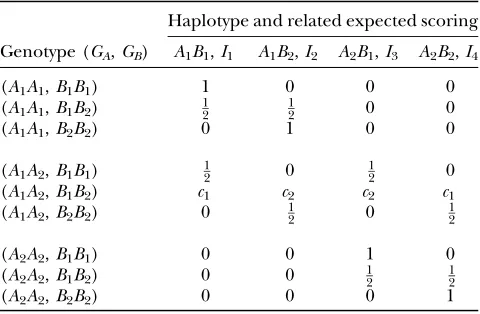
B2. Table 1 gives the score vector for each genotype combination of markers A and B. To understand the entries of Table 1, it is worthwhile to take genotype combination (GA ¼A1A1, GB¼ B1B1) as an example.
Two copies of haplotypeA1B1can be formed from the genotype combination (GA ¼ A1A1, GB ¼ B1B1). The
score for haplotypeA1B1is 1 for this genotype combi-nation; and scores for the other three haplotypes are all 0. Denote the genotype of an individual at markerAby
GAand the genotype at markerBbyGB. Let us denote
c1¼P(A1B1|GA¼A1A2,GB¼B1B2)¼P(A1B1)P(A2B2)/
[2P(A1B1)P(A2B2)1 2P(A1B2)P(A2B1)]¼c4;i.e.,c1is the conditional probability of a haplotype A1B1 given the double heterozygotes (GA¼A1A2,GB¼B1B2); and
c2 ¼c3¼1
2c1: For the double heterozygotes (GA ¼
A1A2,GB¼B1B2), the expected scores arec1,c2,c2,c1for
haplotypes A1B1, A1B2, A2B1, A2B2. The scores of the other genotype combinations are provided in Table 1. Then the corresponding model of the haplotype trend regression method can be written as
y¼wg1X 4
i¼1
Iibi1e; ð17Þ
wherebiare regression coefficients, andIiare expected
scorings of haplotypes defined in Table 1. It can be seen that model (17) is not equivalent to either proposed model (13) or model (14).
In the general case of M markers, let Ij be the
expected score of haplotypehj,j¼1, 2,. . . ,J. In terms
of conditional probabilities,Ijcan be expressed as
Ij ¼ X
G1 . . .X
GM
PðhjjG1;. . .;GMÞ1ðG1;...;GMÞ:
TABLE 1
Expected scoringsIi,i¼1, 2, 3, 4 of haplotypes of model (17)
Haplotype and related expected scoring Genotype (GA,GB) A1B1,I1 A1B2,I2 A2B1,I3 A2B2,I4
(A1A1,B1B1) 1 0 0 0
(A1A1,B1B2) 12
1
2 0 0
(A1A1,B2B2) 0 1 0 0
(A1A2,B1B1) 12 0
1
2 0
(A1A2,B1B2) c1 c2 c2 c1
(A1A2,B2B2) 0 12 0 12
(A2A2,B1B1) 0 0 1 0
(A2A2,B1B2) 0 0 12 12 (A2A2,B2B2) 0 0 0 1
The constants are given byc1¼P(A1B1|GA¼A1A2,GB¼B1B2)¼ P(A1B1)P(A2B2)/[2P(A1B1)P(A2B2)12P(A1B2)P(A2B1)] andc2¼
The corresponding model of the haplotype trend re-gression method can be written as
y¼wg1X
J
j¼1
Ijbj1e: ð18Þ
Forj¼1, 2,. . .,J, let us denoteDhjQ ¼PðQ1hjÞ q1Phj,
which are measures of LD between QTL Q and the haplotypes. HereP(Q1hj) is the frequency of haplotype
Q1hj. In appendix f, we show that the regression
co-efficients of model (18) satisfy the matrix equation
EðI12Þ EðI1I2Þ . . . EðI1IJÞ
EðI2I1Þ EðI22Þ . . . EðI2IJÞ ..
.
.. .
. . . ...
EðIJI1Þ EðIJI2Þ . . . EðIJ2Þ 0 B B B B B @ 1 C C C C C A b1 b2 .. . bJ 0 B B B B B @ 1 C C C C C A ¼m Ph1 Ph2 .. .
PhJ
0 B B B B B @ 1 C C C C C A
1 aQ
a1 a2 .. . aJ 0 B B B B @ 1 C C C C
A dQ
d1 d2 .. . dJ 0 B B B B @ 1 C C C C A; ð19Þ
whereE(IiIk) are given inappendix f, and
aj¼ X
G1 . . .X
GM
PðhjjG1;. . .;GMÞ
3 X
J
i¼1
XJ
k¼1
PðG1;. . .;GMjhi;hkÞPhiDhkQ1PhkDhiQ
dj¼ X
G1 . . .X
GM
PðhjjG1;. . .;GMÞ
3 X
J
i¼1
XJ
k¼1
PðG1;. . .;GMjhi;hkÞDhiQDhkQ:
From Equations 19, it is clear that model (18) models both the additive and dominance effects. Suppose that the haplotype and the QTLQ are in linkage equilib-rium;i.e.,DhjQ ¼0;j¼1;2;. . .;J. Then Equation 19
im-pliesb1¼ ¼bJ ¼m, since
PJ
j¼1Ij ¼1 andEIj¼Phj.
Hence, model (18) is reduced to (5). To test association between the haplotypes and the trait locus, one may test a null hypothesisb1 ¼ ¼bJ, and the relatedF-test
statistic can be constructed.
Again, assume thatN individuals from a population are available for study with trait values and genotype information. On the basis of regression (18), one may construct anF-test statisticFHTRto test the null hypoth-esisb1¼ ¼bJ¼m(Graybill1976). Under the null
hypothesis,FHTRis central toF(J1,NJ). Under the alternative hypothesis that at least twobj’s are not equal
to each other, FHTR is noncentral toF(J 1,N J). Assume the sample sizeNis large enough that the large sample theory applies. Then it can be shown that the
corresponding noncentrality parameter is approxi-mated by
lHTRN
s2ðb1b2;. . .;b1bJÞ½HE
1Ht1 3ðb1b2;. . .;b1bJÞt;
where
E ¼
EðI12Þ EðI1I2Þ . . . EðI1IJÞ
EðI2I1Þ EðI22Þ . . . EðI2IJÞ ..
.
.. .
. . . ...
EðIJI1Þ EðIJI2Þ . . . EðIJ2Þ 0 B B B B B @ 1 C C C C C A H ¼
1 1 0 0 . . . 0 0 0
1 0 1 0 . . . 0 0 0
1 0 0 1 . . . 0 0 0
.. . .. . .. . .. . . . . ... ... ...
1 0 0 0 . . . 0 1 0
1 0 0 0 . . . 0 0 1
0 B B B B B B B B B @ 1 C C C C C C C C C A
ðJ1Þ3J :
The advantage of model (17) is that it may model the haplotype effect by parameters bi. In practice, it is
necessary to calculate the expected scorings or haplo-type frequencies before building the haplohaplo-type trend regression model. Instead, the proposed models (13) and (14) may be used to analyze genetic data directly. Moreover, we have derived analytical formulas to calcu-late the regression coefficients of the HTR method and the related noncentrality parameter of the test statistic
FHTR. Note that the original article by Zaykin et al.
(2002) did not work out this very useful information. Our analytical coefficient equations and related non-centrality parameter approximations can be readily uti-lized for power evaluation.
RESULTS
Type I error rates:To evaluate the robustness of the proposed models, we calculate type I error rates of test statistics Fm,ad, Fm,a, FAB,ad, FAB,a, and FHTR at a 0.05
significance level. The results are presented in Tables 2 and 3. Four test cases are considered: null, no major gene effect a ¼ d ¼ 0; additive, additive mode of in-heritance a ¼1, but no dominant effect d ¼0; dom-inant, dominant mode of inheritance a ¼d ¼1; and recessive, recessive mode of inheritancea¼1 andd¼ 0.5. The total variance is fixed ass2¼1.0 and the trait
PA1 ¼ ¼PA4 ¼0:25 when m¼4; PA1¼ ¼PA5 ¼ 0:2 whenm¼5; andPA1¼PA2 ¼0:2;PA3¼ ¼PA6 ¼ 0:15 whenm¼6.
To calculate the type I error rates, 10,000 data sets are simulated for each test case. Each data set contains either 200 or 300 individuals. In each test case in Table 2, the data sets are generated under an assumption of linkage equilibrium between the QTLQand the markerA;i.e.,
DAiQ ¼PðQ1AiÞ q1PAi ¼0. That is, there is no
associa-tion between the QTLQand markerA. Utilizing the data
sets, we fit either model (8) or model (9), and then calculate theF-testFm,adorFm,a. Because the data sets are
generated under the assumption of linkage equilibrium, an empirical test statistic that is larger than the cutting point of the relatedF-statistic at a 0.05 significance level is treated as a false positive. On the basis of theF-test of eitherFm,adorFm,a, type I error rates are calculated as the
proportions of the 10,000 simulation data sets that give significant results at the 0.05 significance level.
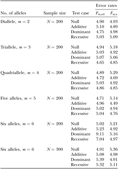
For the test statisticFm,a, the Table 2 results show that
the type I error rates are around the 0.05 nominal sig-nificance level in all cases. Hence, the proposed model (9) is robust for data sets of a sample sizeN¼200. For test statisticFm,ad, the type I error rates are around the
0.05 nominal significance level whenm#5 for data sets of sample sizeN¼200. Form¼6 and a sample sizeN¼ 200, the type I error rates of testFm,ad are too big for
the dominant and recessive test cases (9.11 and 7.04%, respectively). This is partially due to the large degrees of freedom, JA 1 ¼ m(m 1 1)/2 1 ¼ 20 of test
Fm,adwhen m¼6; in addition, the high rate of type I
error may be also caused by the mode of inheritance,
i.e., for the cases of dominant and recessive models. When the sample size increases toN¼300, the type I error rates of test Fm,ad are around the 0.05 nominal
significance level form¼6. Model (8) is less robust than model (9).
In Table 3, two markersAandBare used in the anal-ysis. The numbersmandnof alleles are equal to 2. The allele frequencies are given by PA1¼PA2 ¼0:5 and PB1¼PB2¼0:5. In each test case, linkage equilibrium is assumed between the QTLQand the markersAandB;
i.e.,DAiQ ¼DBiQ ¼0. DenoteDA1B1 ¼PðA1B1Þ PA1PB1, which is the measure of LD between A and B. Here
P(A1B1) is the frequency of haplotypeA1B1. Let
DAQB ¼PðA1Q1B1Þ PA1DB1Qq1DA1B1PB1DA1QPA1q1PB1 ð20Þ
be the measure of the third-order LD (Thomson
and Baur 1984). Here P(A1Q1B1) is the frequency of
haplotypeA1Q1B1. Between markerAand markerB, two situations are considered: (1) linkage equilibrium,i.e.,
DA1B1 ¼0, and (2) linkage disequilibrium,i.e.,DA1B1¼ 0:08. No linkage disequilibrium of third order is assumed among markersAandBand the QTLQ; that is,DAQB¼0. Again, 10,000 data sets are simulated for
each test case, and each data set contains 200 individ-uals. The simulation is done as follows. First, the haplotype frequencies are calculated on the basis of allele frequencies and LD coefficients by relation (20) (Thomsonand Baur1984). Then data sets are
simu-lated using the haplotype frequencies. On the basis of theF-test of eitherFAB,ador FAB,a or the HTR method,
type I error rates are calculated as the proportions of the 10,000 simulation data sets that give significant results at the 0.05 significance level. The Table 3 results show that the type I error rates are around the 0.05 nominal
TABLE 2
Type I error rates (percentage) of test statisticsFm,adandFm,a
at a 0.05 significance level when only one markerAis used
in the analysis
Error rates No. of alleles Sample size Test case Fm,ad Fm,a
Diallele,m¼2 N¼200 Null 4.90 4.93 Additive 5.10 4.89 Dominant 4.75 4.98 Recessive 5.03 5.09
Triallele,m¼3 N¼200 Null 4.94 5.18 Additive 5.03 4.92 Dominant 5.07 5.06 Recessive 4.65 4.85
Quadriallele,m¼4 N¼200 Null 4.89 5.29 Additive 4.72 4.69 Dominant 5.03 4.92 Recessive 4.86 4.85
Five alleles,m¼5 N¼200 Null 4.71 5.14 Additive 4.96 4.49 Dominant 5.02 4.94 Recessive 5.04 4.76
Six alleles,m¼6 N¼200 Null 5.02 5.21 Additive 5.23 4.92 Dominant 9.11 5.16 Recessive 7.04 4.97
Six alleles,m¼6 N¼300 Null 4.91 5.36 Additive 5.08 4.98 Dominant 5.39 4.91 Recessive 5.32 5.11 The total variance is fixed ass2¼ 1.0 and the trait allele
frequency is taken asq1¼q2¼0.5. The numbermof alleles
ranges from 2 to 6. The allele frequencies are given by:
PA1 ¼PA2 ¼0:5 whenm¼2;PA1 ¼0:4;PA2¼PA3 ¼0:3 when
m ¼ 3; PA1¼ ¼PA4 ¼0:25 when m ¼ 4; PA1 ¼ ¼
PA5 ¼0:2 when m ¼ 5; and PA1¼PA2 ¼0:2;PA3 ¼ ¼
significance level in all cases. Hence, the proposed models (13) and (14) and the HTR method are robust for data sets of a sample sizeN¼200.
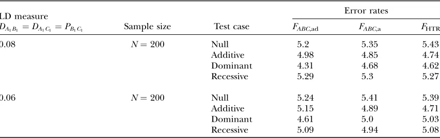
Table 4 shows type I error rates (percentages) of test statisticsFABC,ad,FABC,a, andFHTRat a 0.05 significance
level when three diallelic markersA,B, andCare used in the analysis. The measuresDABC,DAQC, andDBQCof the
third-order LD are defined as that ofDAQB; the measure
of the fourth order is defined accordingly (Bennett
1954). Such as relation (20), the haplotype frequencies
at the three markers A, B, and C and at QTL Q are calculated on the basis of allele frequencies and LD co-efficients by Weir’s(1996, p. 119) relation (3.14). Then
data sets are simulated using the haplotype frequencies. Since this article is about population data, one indi-vidual may have two copies of haplotypes. Each haplo-type is sampled according to the haplohaplo-type frequencies. From the Table 4 results, we can see that the proposed models and the HTR method give correct type I errors for data sets of a sample sizeN¼200.
TABLE 3
Type I error rates (percentage) of test statisticsFAB,ad,FAB,a, andFHTRof the haplotype trend regression (HTR)
method at a 0.05 significance level when two markersAandBare used in the analysis
LD measure
DA1B1 ¼PðA1B1Þ PA1PB1
Error Rates
Sample size Test case FAB,ad FAB,a FHTR
0 N¼200 Null 4.90 5.22 5.39
Additive 5.09 4.75 4.77 Dominant 4.62 4.87 4.79 Recessive 5.36 5.12 4.81
0.08 N¼200 Null 5.09 5.23 5.55
Additive 4.92 4.74 4.71 Dominant 4.63 4.84 4.71 Recessive 5.04 5.02 4.94 The total variance is fixed ass2¼1.0 and the trait allele frequency is taken asq
1¼q2¼0.5. The numbersm
andnof alleles¼2. The allele frequencies are given byPA1 ¼PA2¼0:5 andPB1 ¼PB2 ¼0:5. Four test cases are considered: null, no major gene effecta¼d¼0; additive, additive mode of inheritancea¼1, but no dominant effectd¼0; dominant, dominant mode of inheritancea¼d¼1; recessive, recessive mode of inheritancea¼1 andd¼–0.5. In each test case, linkage equilibrium is assumed between the QTLQand the markersAandB;i.e.,
DAiQ ¼DBiQ ¼0. No linkage disequilibrium of third order is assumed among markersAandBand the QTLQ;
that is,DAQB¼0.
TABLE 4
Type I error rates (percentage) of test statisticsFABC,ad,FABC,a, andFHTRof the haplotype trend regression
(HTR) method at a 0.05 significance level when three diallelic markersA,B, andCare used in the analysis
LD measure
DA1B1 ¼DA1C1 ¼PB1C1
Error rates
Sample size Test case FABC,ad FABC,a FHTR
0.08 N¼200 Null 5.2 5.35 5.43
Additive 4.98 4.85 4.74 Dominant 4.31 4.68 4.62 Recessive 5.29 5.3 5.27
0.06 N¼200 Null 5.24 5.41 5.39
Additive 5.15 4.89 4.71 Dominant 4.61 5.0 5.03 Recessive 5.09 4.94 5.08 The total variance is fixed ass2¼1.0 and the trait allele frequency is taken asq
1¼q2¼0.5. The allele
fre-quencies are given byPA1 ¼PA2¼0:5,PB1 ¼PB2 ¼0:5, andPC1 ¼PC2¼0:5. Four test cases are considered: null, no major gene effecta¼d¼0; additive, additive mode of inheritancea¼1, but no dominant effectd¼0; dominant, dominant mode of inheritancea¼d¼1; recessive, recessive mode of inheritancea¼1 andd¼–0.5. In each test case, linkage equilibrium is assumed between the QTL Q and the markers A, B, and C; i.e.,
DAiQ ¼DBiQ ¼DCiQ ¼0. Moreover, neither third- nor fourth-order linkage disequilibrium is assumed;i.e.,DABC¼
Power calculation and comparison: Leth2¼s
ga
2 /s2
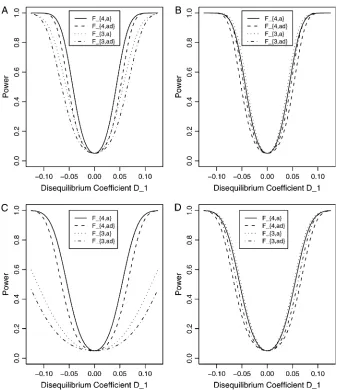
be the heritability. Figure 1 shows power curves of the test statistics F4,a, F4,ad, F2,a, and F2,ad against the dis-equilibrium coefficientDA1Qfor a dominant mode of in-heritancea¼d¼1.0 at a 0.05 significance level based on the approximations of noncentrality parameters lm,a
and lm,ad. F4,a and F4,ad are calculated when A has
four equal frequency alleles;i.e.,PA1 ¼ ¼PA4¼0:25. In addition, the measures of LD are given as follows: Figure 1, A and B,DA2Q ¼DA4Q ¼ DA1Q;DA3Q ¼DA1Q, and Figure 1, C and D,DA2Q ¼ DA1Q;DA3Q ¼ DA4Q ¼ DA1Q=2.F2,a and F2,adare calculated by collapsing the four alleles to be two alleles: in Figure 1, A and C, alleles
A1andA2are collapsed as one allele, and allelesA3and
A4are collapsed to be the other; in Figure 1, B and D, alleles A1 and A3 are collapsed to be one allele, and allelesA2andA4are collapsed to be the other. ForF2,a
andF2,ad, a simple calculation can show that the mea-sures of LD in Figure 1A are 0, 0; the meamea-sures of LD in Figure 1B are 2DA1Q;2DA1Q; the measures of LD in Figure 1C are 0, 0; and the measures of LD in Figure 1D are 3DA1Q=2;3DA1Q=2. Hence, the QTLQis in linkage equilibrium with the marker after collapsing the alleles
in Figure 1, A and C. The other parameters areq1¼0.50,
h2¼0.25,N¼200.
From Figure 1, we may see the following:
1. F4,ad is slightly less powerful than F4,a, and F2,ad is slightly less powerful thanF2,a. This is because that test statistic Fm,ad has larger degrees of freedom
than those ofFm,a. Note that the noncentrality
param-eter approximationlm,adofFm,adis given by Equation
10. The contribution of the dominance effect is
Ns2 gdRAQ4 =s
2; which depends on both dominance
effectdand the magnitude of factorR4
AQ;and it can
be significant when both of them are large enough. Hence, including a dominance component in the model can improve the power of QTL detection only when the magnitude of s2
gdR 4
AQ is large enough to
compensate for the extra degrees of freedom. Note that the quantitys2
gdR 4
AQ is the product of the
dom-inance variances2
gdand of the measureRAQ4 of LD.
The magnitude of s2 gdR
4
AQ is the result of the
dominance variance s2
gd reduced by a factor R 4
AQ:
Even whens2
gdis large,s 2 gdR
4
AQcan be small when LD
coefficients are not big;i.e.,R4
AQ is small.
Figure1.—Power curves of the test
statis-ticsF4,ad,F4,a,F2,ad, andF2,aagainst the
dis-equilibrium coefficient D1¼DA1Q for a dominant mode of inheritancea¼d¼1.0 at a 0.05 significance level.F4,adandF4,aare
calculated when markerAhas four equal fre-quency alleles; i.e., PA1¼ ¼PA4 ¼0:25. The measures of LD are (A and B)DA2Q¼
DA4Q¼ DA1Q;DA3Q¼DA1Q and (C and D)
DA2Q¼DA1Q;DA3Q¼DA4Q ¼DA1Q=2.F2,ad
andF2,aare calculated by collapsing two of
the four alleles: (A and C) allelesA1andA2
are collapsed as one allele, and allelesA3
and A4 are collapsed to be the other; (B
and D) allelesA1andA3are collapsed to be
one allele, and allelesA2andA4are collapsed
to be the other. The other parameters are
2. When the measures of LD are high, the power of the test statistics is high. On the other hand, the power is minimal if all measures of LD are close to 0.
3. The dependence of power on measures of LD can also be observed by comparing Figure 1A with Figure 1C, 1B with 1D. The power ofF4,adandF4,ain Figure 1A is higher than that ofF4,adandF4,ain Figure 1C, respectively; the power of each test statistic in Figure 1B is higher than that of the same test statistic in Figure 1D. This is because the measures of LD in Figure 1A are equal to or higher than those in Figure 1C, and the measures of LD in Figure 1B are equal to or higher than those in Figure 1D.
4. In Figure 1B and Figure 1D, the power of F4,ad is slightly lower than that of F2,ad; the power ofF4,ais slightly lower than that ofF2,a.
5. In Figure 1A and Figure 1C, the power of F2,ad
and F2,a is minimal. This is because measures of LD are 0 after collapsing the alleles in these two graphs.
Figure 2 shows power curves of the test statisticsF4,a,
F4,ad, F3,a, and F3,ad against the disequilibrium
coeffi-cientDA1Q for a dominant mode of inheritancea¼d¼ 1.0 at a 0.05 significance level. F4,a and F4,ad are cal-culated as those in Figure 1.F3,aandF3,adare calculated by collapsing two of the four alleles to be a new alelle: in Figure 2, A and C, alleles A1andA2are collapsed as a new one; in Figure 2, B and D, alleles A1and A3are collapsed to be a new one. For F3,aandF3,ad, a simple calculation can show that the measures of LD in Figure 2A are 0;DA1Q;DA1Q;the measures of LD in Figure 2B are 2DA1Q;DA1Q;DA1Q;the measures of LD in Figure 2C are 0;DA1Q=2;DA1Q=2;and the measures of LD in Figure 2D are 3DA1Q=2;DA1Q;DA1Q=2. Among the features shown in Figure 1, it can be seen that in Figure 2, A and C, the power ofF4,adis higher than that ofF3,ad, and the power ofF4,ais higher than that ofF3,a. In Figure 2, B and D, the power ofF4,adis slightly lower than that of
F3,ad, and the power ofF4,ais slightly lower than that of
F3,a. Hence, the way to collapse the alleles has impact on power.
From Figures 1 and 2, we may see that the power of F4,a and F4,adis relatively stable although it may be slightly lower than that of F3,a, F3,ad, F2,a, and F2,ad in
Figure 2.—Power curves of the test
statisticsF4,a,F4,ad,F3,a, andF3,ad, against
the disequilibrium coefficient D1¼ DA1Q for a dominant mode of inheri-tancea¼d¼1.0 at a 0.05 significance level.F4,adandF4,aare calculated when
marker Ahas four equal frequency al-leles; i.e., PA1 ¼ ¼PA4 ¼0:25. The measures of LD are the same as those in Figure 1.F3,adandF3,aare calculated
by collapsing two of the four alleles: (A and C) allelesA1andA2are collapsed as
a new one; (B and D) allelesA1andA3
are collapsed to be a new one. The other parameters areq1¼0.50,h2¼0.25,N¼
certain circumstances. However, the power ofF3,a,F3,ad,
F2,a, andF2,addepends heavily on the way to collapse the alleles. This shows the advantage of using multiallelic markers in an association study of QTL detection. For multiallelic marker data, the proposed test statistics
Fm,a and Fm,ad can be directly used to test if there is
association between the marker and the QTL. As shown in Figures 1 and 2, the test statisticFm,ais usually more
powerful thanFm,ad due to the increase of degrees of
freedom of test statisticFm,ad.
Figure 3 shows power curves of the test statisticsF4,a
andF4,adagainst the heritabilityh2at a 0.05 significance
level for a dominant mode of inheritancea¼d¼1.0 and for a recessive mode of inheritance a ¼1.0, d ¼ 0.5, respectively. As with Figures 1 and 2, Figure 3 is based on noncentrality parameter approximations (10) and (11). In Figure 3, A and B, the power can be high as the heritabilityh2.0.1; in these two graphs, the
mea-sures of LD are given by DA1Q ¼ DA2Q ¼DA3Q ¼ DA4Q ¼0:08. In Figure 3, C and D, the power can be high as the heritabilityh2.0.15; in these two graphs, the
measures of LD are given byDA1Q ¼ DA2Q ¼DA3Q ¼ DA4Q ¼0:06. Figure 4 shows power curves of the test
statisticsF4,aandF4,adagainst the trait allele frequencyq1
or marker allele frequency PA1 at a 0.05 significance level. It can be seen that the power depends on both the measures of linkage disequilibrium and the trait allele frequencyq1or marker allele frequencyPA1.
Comparison with the haplotype trend regression method:Assume that the two diallelic markersAandB
are used in the analysis. Figures 5 and 6 show power curves of the test statisticsFAB,a,FHTR, andFAB,adagainst
the heritabilityh2at a 0.05 significance level. The related
parameters are given in the figure legends. The power curves of the test statistics FAB,a, FHTR, and FAB,ad are
calculated on the basis of approximations of noncen-trality parameterslABa,lHTR, andlABad.
In Figure 5, no third-order linkage disequilibrium is assumed;i.e.,DAQB¼0. In Figure 6, A and B, weak
third-order linkage disequilibrium is assumed; i.e., DAQB ¼
0.025. It can be seen that the genotype effect model can be less powerful than the HTR method, and the HTR method can be less powerful than the additive effect model in the case of no or weak third-order linkage disequilibrium among the two markers and the QTL (Figure 5 and Figure 6, A and B). In Figure 6, C and D,
Figure3.—Power curves of the test
sta-tisticsF4,aandF4,adagainst the heritability h2at a 0.05 significance level. (A and C)
The curves are plotted for a dominant mode of inheritance a ¼ d ¼ 1.0; (B and D) the curves are plotted for a reces-sive mode of inheritance a ¼ 1.0, d ¼ 0.5. F4,a and F4,ad are calculated when
marker A has four equal frequency al-leles;i.e.,PA1¼ ¼PA4 ¼0:25. The mea-sures of LD are given as follows: (A and B)
strong third-order linkage disequilibrium is assumed;
i.e.,DAQB ¼0.065. In the case that strong third-order
linkage disequilibrium exists, the HTR method can be more powerful (Figure 6, C and D).
Note the following fact: in Figure 6, A and B, the max-imum ofDAQBis 0.025; in Figure 6, C and D, the
max-imum ofDAQBis 0.065 (otherwise, some of the haplotype
would have negative frequencies). Thus, the simulated power curves of the haplotype trend regression method in Figures 5 and 6 represent the two extreme situations: (1) no third-order linkage disequilibrium (Figure 5) and (2) strongest third-order linkage disequilibrium (Figure 6). In practice, the third-order linkage disequi-librium would exist in a more moderate way that is between the two extremes; and the power of the hap-lotype trend regression method should be between those of the two extremes. Note that the proposed geno-type effect model and additive effect model utilize only the second-order linkage disequilibrium or pairwise linkage disequilibrium. Hence, the powers ofFAB,aand FAB,adare the same for Figures 5 and 6.
Figure 7 shows power curves of the test statisticsFABC,a
andFABC,adandFHTRagainst the heritabilityh2at a 0.05
significance level, when three diallelic markersA,B, and
C are used in the analysis. The related parameters are given in the figure legend. From Figure 7, it can be seen that the power ofFHTRis the lowest. This is due to the large number of degrees of freedom ofFHTR, which is
F(7,N8),N¼200. In contrast,FABC,aisF(3,N4), N¼200; andFABC,aisF(6,N7),N¼200. The low power
ofFHTRis most likely due to the biallelic QTL situation that we consider. In the situation of multiple QTL haplotypes and strong LD between QTL and marker haplotypes, the haplotype-based methods are expected to have good power.
Comparison based on ACE haplotype frequencies: To work on more realistic scenarios, we take the hap-lotype information of ACE genes as an example. Ten diallelic polymorphisms in the ACE gene spanning 26 kb were genotyped (Keavneyet al.1998). The order
of the 10 polymorphisms is T-5991C, A-5466C, T-3892C, A-240T, T-93C, T1237C, G2215A, I/D, G2350A, and 4656(CT)3/2. Table 5 lists 10 haplotypes, where the first 7 are the most frequent haplotypes (http://www.well. ox.ac.uk/mfarrall/oxhap_freq.html). For the 10 hap-lotypes, allele I at marker I/D is always present with allele A at marker G2350A, and allele D at marker I/D is always present with allele G at marker G2350A. Hence,
Figure4.—Power curves of the test
statisticsF4,aandF4,adagainst the trait
allele frequencyq1or allele frequency PA1 at a 0.05 significance level. (A and C) The curves are plotted for a domi-nant mode of inheritancea¼d¼1.0; (B and D) the curves are plotted for a recessive mode of inheritancea¼1.0,
d¼ 0.5. (A and B) The parameters are given by PA1 ¼ ¼PA4 ¼0:25,
q2 ¼ 1q1;DA1Q¼ ðminðq1;PA1Þ q1 PA1Þ=2¼ DA2Q¼DA3Q ¼ DA4Q; (C and D) the parameters are given by
PA2¼0:5PA1, PA3¼PA4¼0:25;q1¼
the two markers can be treated as one. Similarly, mark-ers T-5991C and A-5466C can be treated as one; and markers A-240T and T-93C can be treated as one. There-fore, the 10 haplotypes can be considered as containing seven markers.
In Abecasiset al.(2000a,b) and Fanet al.(2005), it is
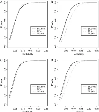
found that that markers I/D and G2350A show strongest association with the circulating ACE level. Thus, markers I/D and G2350A are treated as a putative trait locusQ. A quantitative trait of the putative locusQis simulated for each graph in Figure 8, A–D. The empirical power curves of the test statisticsFHTR,Fa, andFadare plotted against the heritabilityh2at a 0.05 significance level in
Figure 8. HereFais the test statistic based on the additive effect model, andFad is the test statistic based on the genotype effect model. The empirical power curves
SFHTR,SFa, andSFadin Figure 8 are calculated as follows. First, the interval (0.01, 0.25) of the heritability h2 is
divided into 24 subintervals. Correspondingly, the 24 subintervals lead to 25 end points. For each end point, there is a set of parameters for the power curve. Using the set of parameters, 2500 data sets are simulated for each end point. For each data set, empirical statistics ofFHTR,
Fa, and Fad are calculated. The simulated power is the proportion of the 2500 simulated data sets for which the empirical statistic is larger than the cutting point of the corresponding F-distribution at a 0.05 significance level.
In Figure 8, A and C, the curves are plotted for a dominant mode of inheritancea¼d¼1.0; in Figure 8, B and D, the curves are plotted for an additive mode of inheritancea¼1.0,d¼0. In Figure 8, A and B, all 10 haplotypes are used in the simulations; in Figure 8, C and D, only the first 7 most frequent haplotypes are used. From Figure 8, A–D, it can be seen that the proposed additive effect model has similar power to that of the HTR method. In Figure 8, A and C, when the dominance effects are present, the genotype effect model has similar power to those of the additive effect model and the HTR method. In Figure 8, B and D, the genotype effect model is less powerful because of the absence of the dominance effect. Hence, the genotype effect model can be useful only if the dominance effect can compensate for the extra degrees of freedom.
Simulation study: To evaluate the accuracy of the noncentrality parameter approximations, we performed
Figure5.—Power curves of the test
sta-tisticsFAB,aandFAB,adandFHTRof the
hap-lotype trend regression method against the heritability h2 at a 0.05 significance
level, when two diallelic markersAandB
are used in the analysis. (A and C) The curves are plotted for a dominant mode of inheritancea¼d¼1.0; (B and D) the curves are plotted for an additive mode of inheritancea¼1.0,d¼0. (A and B) The parameters are given by DA1Q¼
DB1Q ¼0:15;DA1B1 ¼ 0:10;DA1QB1 ¼0; (C and D) the parameters are given by
DA1Q¼DB1Q¼0:10;DA1B1¼0:08;DA1QB1¼ 0. The other parameters arePA1¼PA2¼
simulations for the power curves in Figures 1, 2, 5, 6, and 7. The results are presented as supplemental in-formation (http://www.genetics.org/supplemental/). It can be seen that the approximations are excellent.
DISCUSSION
In this article, two models, the genotype effect model and the additive effect model, are proposed for high-resolution association mapping of QTL on the basis of population data. The two models extend our previous research, which is based on multiple diallelic markers (Fan and Xiong 2002, 2003; Jung et al. 2005). The
genotype effect model is closely linked to the measured genotype approach (Boerwinkleet al.1986). The very
popular genetics software such as Mendel 5.0 is already capable of performing association mapping of QTL by the additive effect model (Cantoret al. 2005; Lange et al.2005). Surprisingly, there is no research to theoreti-cally show why these two models are valid methods in association mapping of QTL under normal distribution. There are no existing analytical formulas to evaluate the power of the related test statistics. This article shows that
the model coefficients are functions of measures of LD; and thus relatedF-test statistics can be constructed for association study of QTL. In the presence of both additive and dominance effects of the QTL, either the
Fm,ad(orFAB,ad) statistic or theFm,a(orFAB,a) statistic can
be used. Since the Fm,ad (or FAB,ad) test statistic has
bigger degrees of freedom than those ofFm,a(orFAB,a), Fm,a(orFAB,a) can be more powerful. If the extra degrees
of freedom of the Fm,ad test can be compensated by
magnitudes2
gdRAQ4 ;it can be more powerful thanFm,a.
The formulas of noncentrality parameter approxima-tions (10) and (11) clearly indicate the dependence of the power on the quantityRAQ2 for genetic data. That is,
the noncentrality parameter of test statistics of the null hypothesis of no genetic effects is reduced by a factor ofR2
AQ for additive variance and by a factor ofR
4
AQ for
dominance variance. If only one diallelic marker A is used in the analysis, both our previous research and the work of colleagues have derived similar formulas to sup-port this argument (Shamet al. 2000; Fanand Xiong
2002, 2003; Fan and Jung2003; Fan et al.2005; Jung et al. 2005). This is a good example in the debate on appropriate measures of LD for markers or multiallelic
Figure6.—Power curves of the test
sta-tisticsFAB,aandFAB,adandFHTRof the
hap-lotype trend regression method against the heritability h2 at a 0.05 significance
level, when two diallelic markers A and
markers (Hedrick 1987; Devlin and Risch 1995;
Pritchard and Przeworski 2001; Weiss and Clark
2002). For multiallelic markers or haplotypes, a satisfac-tory measure of LD has not been derived, as mentioned regarding p306 in Ardlieet al.(2002). For two diallelic
lociA and Q, Ardlie et al. (2002) favor using R2
AQ ¼
D2
A1Q=ðPA1PA2q1q2Þ, which is the correlation of alleles at the two loci. For multiallelic marker data, this article extends previous research by providing the definition ofRAQ2 and deriving Equations 10 and 11. Hayeset al.
(2003) introduced a multilocus approach for estimating LD and past effective size and used chromosome seg-ment homozygosity (CSH), which was introduced in Sved(1971). The dependence of the noncentrality
pa-rameter on the quantityR2
AQ has been indicated by our
study and also by Shamet al.(2000).
In Fulker et al. (1999), Abecasis et al. (2000a,b,
2001), and Shamet al.(2000), an association
between-family and association within-between-family (‘‘AbAw’’) approach is proposed to decompose the genetic association into effects of between pairs and within pairs on the basis of variance component models. The AbAw approach is based on any single diallelic marker. Instead of using a single diallelic marker, we have proposed variance
com-ponent models using multiple diallelic markers. In our models, the association is decomposed into additive and dominance components (Fan and Xiong2002, 2003;
Fanand Jung2003; Fanet al.2005; Junget al.2005). In
Fanand Jung(2003), Fanet al.(2005), and Junget al.
(2005), we compare our method with the AbAw ap-proach and find that our method is advantageous over the AbAw approach. In model (1) or (2), only one marker is used in model building. If multiple markers or multiallelic markers are available, it is very easy to generalize the models to analyze the data. For instance, model (14) generalizes model (1) if two markers are available in the analysis. Accordingly, model (13) gen-eralizes model (2). If only one marker is used in analysis, the proposed model (2) is equivalent to the haplotype trend regression method by Zaykinet al.(2002), which
is very close to the method of Schaidet al.(2002).
How-ever, the proposed models are different from the haplo-type trend regression method for two/multiple marker data. If both markers are diallelic markers, the genotype effect model can be less powerful than the HTR method, and the HTR method can be less powerful than the additive effect model in the case of no or weak third-order linkage disequilibrium among the two markers and the
Figure7.—Power curves of the test
sta-tisticsFABC,aand FABC,adandFHTRof the
haplotype trend regression method against the heritabilityh2at a 0.05
signif-icance level, when three diallelic markers
A, B, and C are used in the analysis. (A and C) The curves are plotted for a dom-inant mode of inheritancea¼d¼1.0; (B and D) the curves are plotted for an ad-ditive mode of inheritancea¼1.0,d¼0. (A and B) The parameters are given by
DAQ ¼ DBQ ¼DCQ ¼DDQ¼ 0.12,DAB¼
DAC¼DBC¼0.08; (C and D) the param-eters are given byDAQ ¼ DBQ ¼ DCQ ¼
DDQ¼0.10,DAB¼DAC¼DBC¼0.06. Nei-ther third- nor fourth-order linkage dis-equilibrium is assumed among markers and the QTL. The other parameters are
QTL. If strong third-order linkage disequilibrium exists, the HTR method can be more powerful.
Basically, the proposed models are genotype based. The models can be used to analyze directly any num-ber of markers, and the markers can be either diallelic or multiallelic. By a simulation study based on ACE haplotype frequencies, we show that the proposed additive effect models have similar power to that of the
haplotype-based HTR method. In the meantime, the proposed models enjoy the simplicity of not needing to estimate the expected haplotype scorings; in contrast, the HTR method needs to calculate the expected hap-lotype scorings before building the models. The pro-posed models decompose the main marker effects into a summation of additive and dominance effects. In the presence of haplotype effects, it is important to estimate the haplotype effects and haplotype-based methods are more relevant (Stramet al.2003; Tregouetet al.2004).
One potential problem of this generalization is that the number of parameters can be very big. Then, one needs to select important alleles in the analysis and search for important genetic variants that are truly asso-ciated with the genetic traits. At first glance, model (1), (2), (13), or (14) seems too complicated and contains too many terms. However, the models are not inti-midating at all if one takes into account the recent discovery of haplotype structure in the human genome. Although a haplotype block may contain many SNPs, it takes only a few SNPs to uniquely identify each of the haplotypes in the block. Within a block, there are only two to four common haplotypes (Arnheimet al.2003;
Daly et al. 2001; Goldstein 2001; Patil et al. 2001;
TABLE 5
Ranked ACE haplotype frequencies
Haplotype rank
Haplotype identity
Haplotype
code Frequency
1 TATATTGIA3 1111112111 0.352113 2 CCCTCCADG2 2222221222 0.284507 3 TATATCADG2 1111121222 0.087324 4 TACATCADG2 1121121222 0.073239 5 TATATCGIA3 1111122111 0.050704 6 CCCTCCGDG2 2222222222 0.025352 7 TATATTAIA3 1111111111 0.025352 8 CCCTCCGIA3 2222222111 0.008451 9 CCCTCCADG3 2222221221 0.008451 10 TATATCGDG2 1111122222 0.008451
Figure8.—Empirical power curves of
the test statisticsFHTR,Fa, andFadagainst
the heritability h2 at a 0.05 significance
level. The notation SFa is the empirical
power of theF-test statistic based on the additive effect model,SFadis the
empiri-cal power of theF-test statistic based on the genotype effect model, andSFHTRis