R E S E A R C H
Open Access
Non-integer expansion embedding
techniques for reversible image watermarking
Shijun Xiang
*and Yi Wang
Abstract
This work aims at reducing the embedding distortion of prediction-error expansion (PE)-based reversible watermarking. In the classical PE embedding method proposed by Thodi and Rodriguez, the predicted value is rounded to integer number for integer prediction-error expansion (IPE) embedding. The rounding operation makes a constraint on a predictor’s performance. In this paper, we propose a non-integer PE (NIPE) embedding approach, which can proceed non-integer prediction errors for embedding data into an audio or image file by only expanding integer element of a prediction error while keeping its fractional element unchanged. The advantage of the NIPE embedding technique is that the NIPE technique can really bring a predictor into full play by estimating a sample/pixel in a noncausal way in a single pass since there is no rounding operation. A new noncausal image prediction method to estimate a pixel with four immediate pixels in a single pass is included in the proposed scheme. The proposed noncausal image predictor can provide better performance than Sachnev et al.’s noncausal double-set prediction method (where data prediction in two passes brings a distortion problem due to the fact that half of the pixels were predicted with the watermarked pixels). In comparison with existing several state-of-the-art works, experimental results have shown that the NIPE technique with the new noncausal prediction strategy can reduce the embedding distortion for the same embedding payload.
Keywords: Reversible watermarking; Non-integer prediction error; Expansion embedding; Noncausal prediction
1 Introduction
Reversible watermarking techniques embed data in a host signal (for example, an audio/image) and allow for the original digital image to be exactly recovered. This is very useful in some applications, especially in medical, military, and legal domains. There are two important requirements for reversible watermarking techniques: 1) a large embed-ding capacity and 2) a low watermark distortion. The two requirements conflict with each other since embed-ding more data into a work will cause bigger distortion. A desirable technique should embed the same capacity with lower distortion or vice versa. During the recent 10 years, the reversible watermarking has been an active research domain. In the literature, several types of reversible water-marking algorithms has been proposed:
• Type I algorithms use modulo-arithmetic-based additive spread frequency techniques [1, 2], some of
*Correspondence: [email protected]
Department of Electronic Engineering, School of Information Science and Technology, Jinan University, Guangzhou 510632, China
which provide robustness but often cause salt-and-pepper artifacts due to the many wrapped around pixel intensity. In this direction, a different approach proposed by Vleeschouwer et al. [3] can reduce the artifacts by using the circular interpolation of the bijective transform of image histogram. Finally, good results are reported by using the integer-to-integer wavelet-based reversible watermarking in [4]. • The direct method to reversible watermarking is to
compress a set of selected features from an image in a lossless way and substitute the selected features with their compressed versions and the watermark data [5–8], referred to as type II algorithms in the literature. In order to ensure the watermark
imperceptivity, the selected features are usually in the least significant bit area, such as the generalized LSB (g-LSB) embedding algorithm [8], which is an extension of the work [5]. Theoretical analysis of reversible watermarking has been presented by Kalker and Willems in [7]. Compared with type I algorithms, type II ones can provide higher payload.
• The third type of reversible watermarking algorithms can be classified as difference expansion (DE) embedding methods, in which a common feature is to use difference operators to create features with a small magnitude, and further expand these features in order to create vacancies for embedding the watermark and the auxiliary information. The DE embedding technique was originally developed by Tian [9] and improved in [10–13]. The capacity in Tian’s method is close to 0.5 bpp in a single pass by using two adjacent pixels as a group. By extending the DE to a generalized integer transform, the auxiliary information can be reduced with groups of three or four pixels [10]. In [11], the sorting step in the wavelet domain was introduced to expand those smaller pixel difference. The DE scheme was introduced for 2-D vector map in [12], and the location map was reduced in [13].
• A fruitful research direction, proposed by Thodi and Rodriguez [14], is prediction-error expansion (PE) embedding technique. Comparing with the DE-based methods, one of the advantages of the PE technique is that it significantly adds the number of the feature elements that expanded for data embedding. The other advantage is that a predictor generates feature elements that are often smaller in magnitude than the feature elements generated by a difference operator. With embedding into each pixel, the PE embedding techniques provided the maximal capacity up to 1 bpp in a single pass. So far, several versions of PE reversible watermarking algorithms have been proposed in [14–19] and others in order to improve the performance of the PE schemes by focusing on the reduction of the size of the auxiliary information (with the use of the sorting and histogram shifting techniques [15]), the reduction of the prediction error (by using multiple predictors [16], the prediction by flooring the average value of the four immediate pixels [15] and adaptive prediction [17]), and the reduction of the embedding distortion (by the pixel selection [17] and the low distortion transform by splitting the difference between the current pixel and its prediction context [18, 19]). These existing PE-based schemes share a common property, that is, the predicted value or its variety was rounded to integer value for expansion embedding.
Reversible watermarking algorithms have also been proposed for digital audio files by expansion embed-ding [20–22]. There are other novel reversible watermark-ing approaches which are worth mentionwatermark-ing, too. Data embedded into the histogram bins has been proposed by Leest et al. in [23]. Additive embedding strategy by combining histogram shifting technique [24] and bilinear
interpolation prediction has been proposed by Chen et al. in [25, 26].
This paper proposes a non-integer PE (NIPE) embed-ding strategy, which can proceed non-integer prediction errors for data embedding by expanding only the integer element of a prediction error while keeping the fractional element unchanged. Furthermore, we propose a new non-causal image prediction method for the NIPE technique. In comparison with the classical PE technique [14], the NIPE strategy has lower embedding distortion for non-integer prediction values by using better predictor. The new predictor can provide better performance than exist-ing causal predictors (such as difference predictor, MED predictor, and GAP) due to the fact that there is no rounding operation in the prediction phase. Compar-ing with Sachnev et al.’s noncausal double-set prediction method [15], the proposed prediction method can fur-ther reduce the prediction errors by predicting data in a single pass (which avoids the distortion problem due to the fact that half of the pixels in the second set predicted with the watermarked pixels in the first set). Experimen-tal results for some standard test images have shown that the proposed NIPE method with the noncausal image pre-dictor can embed more payload for the same watermark distortion.
The outline of this paper is as follows. In the next section, the proposed NIPE embedding technique is intro-duced. This is followed by a description of a new pre-diction strategy and an image predictor. We then address the proposed reversible watermarking scheme and com-pare the proposed prediction method with existing typical predictors. Furthermore, the watermarking scheme’s per-formance is tested against other typical reversible image watermarking works. Finally, we draw the conclusions.
2 Prediction-error expansion embedding
PE embedding is a technique to expand a prediction error to create a vacant position and insert a bit into the vacant position, generally at the least significant bit (LSB). The PE-based scheme was originally developed by Thodi and Rodriguez [14] and later developed by other researchers (such as [16–19]). In these methods, causal predictive methods with only past pixels are often applied so that the predicted value or its variety can be rounded to inte-ger value for inteinte-ger prediction-error expansion (IPE) embedding.
2.1 Classical IPE embedding
In the IPE embedding technique [14], the prediction error is the difference between a pixel intensityyand its esti-mateyˆ(which should be rounded to integer value if it is not), denoted bye = y− ˆy. After embedding a bitw, the watermarked prediction error is
ew=2×e+w, (1)
and the marked pixel intensity is
yw= ˆy+ew= ˆy+2×e+w. (2)
Sinceywis an integer number,yˆandeare required to be integer values for expansion embedding. This is why we denote Thodi and Rodriguez’s method as the IPE embed-ding scheme in this paper. It is worth noting that the condition thatˆyshould be integer makes an undesirable requirement, that is, the prediction context often contains onlycausal pixelsso as to obtain the same predicted value ˆ
yin the decoder.
The hidden bit,w, is extracted from the LSB ofewand the original pixel intensityyis recovered by
w=mod(ew, 2), y= ˆy+
ew
2 , (3)
where mod(ew, 2)is the remainder on division ofewby 2 andew2represents the greatest integer less that or equal to ew2.
2.2 NIPE embedding technique
Sections 2.1 shows that the IPE embedding approach [14] is suffering from an undesired requirement, that is, the prediction value should be rounded to integer number for expansion embedding. This will restrain a predictor’s per-formance since the prediction context is restricted to only causal pixels (past pixels) in order to generate the same predicted value in the decoder. In this section, we propose a new expansion embedding approach, one of the advan-tages of which is able to deal with non-integer prediction values for data embedding. The other, more important, advantage of the approach is that the current pixel can be estimated in a single pass by using noncausal predictive way to improve prediction performance2.
From the expressionyw= ˆy+2×e+win Eq. (2), we find that in order to recover the marked pixelyw, not exact of an integerˆyis needed, but of the sum ofyˆ+2×e. Towards this direction, the basic idea of the proposed approach in this paper is to allowˆyto take non-integer value but make sure that the combination ofyˆandetakes integer value for hiding a given bitw.
For a pixel in intensity y, the prediction error e is a non-integer value when its estimateyˆ takes non-integer number. In this case, split the non-integer error e into two parts: integer part( = fix(e)) and fractional part δ (δ = e−). Here, fix(.) is a function to strip off the fractional part of its argument and returns the integer
part. The function does not perform any form of round-ing or scalround-ing, e.g., fix(−4.4)= −4 and fix(5.4)= 5. The basic idea of the NIPE embedding technique expands only the integer part of a prediction error for data embedding while keeping the fractional part unchanged. The detail is described as follows.
In the encoder, the watermarked prediction error is computed by
ew=
2×+δ+w=e++w, ife≥0
2×+δ−w=e+−w, otherwise , (4)
wherewis a binary bit, taking either 0 or 1. Equation (4) can make sure that the fractional element ofewis equal to that ofe. This is beneficial to recover the watermark bit and the original pixel intensity in the decoder.
The resulting watermarked pixel is
yw= ˆy+ew=
Equation (5) shows that even thoughyˆandetake non-integer values, the watermarked pixel yw is an integer number.
In the decoder, the hidden bitwis extracted fromewand the original pixelyis restored by
w=mod(w, 2), andy= ˆy+fix Take two simple examples to show the proposed NIPE technique:
We can see from these two cases that the NIPE scheme can effectively deal with the non-integer prediction values for reversible watermarking.
2.3 Distortion analysis of NIPE and IPE embedding
Letybe a pixel and letyˆbe an estimate ofycomputed on a neighborhood ofy. Let furtherwis the binary bit to be embedded. Letyw = y+pw, wherepwis the watermark distortion ony. For an image with the same predictor, the embedding distortion from the proposed NIPE scheme is lower than from the classical IPE scheme [14]. This can be explained as follows:
Case 1 yˆis integer: From (2) in the IPE,pw=y− ˆy+w. From (5) in the NIPE,
pw=fix(y− ˆy)+w=y− ˆy+w. In this case,
pw=pw, indicating that the NIPE has the same embedding distortion as the IPE. For example, if
y=100,w= 1,yˆ=102. With NIPE,
pw=fix(100−102)+1= −1; with IPE,
pw=100−102+1=−1;
Case 2 yˆis non-integer andy− ˆy>0: In this case,
pw=y− ˆy +w,
pw=fix(y− ˆy)+w=y−fix(yˆ)−1+w. Since the estimate of a pixelyˆis always positive, we have
pw=y−fix(yˆ)−1+w=y− ˆy −1+w, that is
pw=pw+1, meaning that the IPE scheme will introduce more distortion in this case. For example, ify=100, w=1,yˆ=98.4. With NIPE,
pw=fix(100−98.4)+1=2; With IPE,
pw=100−98+1=3.
Case 3 yˆis non-integer andy− ˆy<0: In this case,
pw=y− ˆy +w. Referring to (5),
pw=fix(y− ˆy)−w=y−fix(yˆ)−w=y−ˆy−w. Fromy− ˆy =pw−w, we havepw=pw−2w, indicating the distortion from the NIPE is higher whenw=1. Whenw=0, the NIPE and IPE has the same embedding distortion. For example, if
y=100,ˆy=101.4. With NIPE,
pw=fix(100−101.4)−w= −1−w; with IPE,
pw=100−101+w=−1 +w. Ifwis 1, then
pw= −2andpw=0; Ifwis 0, then
pw=pw= −1.
In statistics, the predictor error (e=y−ˆy) is equal to the probability of positive or negative and the watermark bit (w) is also equal to the probability of 1 or 0. As a result, the NIPE has the same embedding distortion as the classical IPE scheme (e.g., the same PSNR value).
3 Pixel prediction
Image prediction is an important step in lossless compres-sion coding applications [27–30]. For an image, each pixel is estimated from its neighborhood to generate the pre-diction error. Usually, the mean value and variance of the predicted errors are smaller than that of the original pix-els. This is beneficial to improve coding efficiency. There are two main prediction ways: 1) causal prediction [27, 30]
and 2) noncausal prediction [28, 29]. The main difference between causal and noncausal predictive ways is that the prediction context of the former is restricted to only past pixels while the latter uses past and future pixels. By using causal prediction, the predicted value can be rounded to integer number for enhancing coding efficiency since the prediction context of a pixel has been known, such as the median edge direction (MED) predictor in JPEG-LS standard [30]. Noncausal predictive ways are beneficial to reduce the prediction errors for image vector quantization coding [28, 29] and speech compression [31].
3.1 Image predictors for reversible watermarking
Image prediction is also an important step in the expan-sion embedding-based reversible watermarking [9, 10, 14, 15, 18, 19]. Usually, a better predictor can reduce the pre-diction error for improving the payload capacity with the same embedding distortion. Figure 1 plots four typical prediction operations by estimating the current pixel y
with different neighboring pixels: (a) difference predictor used in [9, 10], (b) MED predictor used in [14, 17–19], (c) the gradient adaptive predictor (GAP) used in [18, 19], and d) prediction with four immediate pixels used in [15, 26]. As shown in Fig. 1, data prediction in the difference pre-dictor, MED prepre-dictor, and GAP is restricted only causal pixels while scanning an image in a raster order. The pre-dictor plotted in Fig. 1d is a noncausal predictive method using four immediate pixels of the current pixel as the context, including two past pixels, and two future pixels.
In the DE-based reversible watermarking [9], the differ-ence of two adjacent pixels is expanded to create space to embed the data and the auxiliary information. The aux-iliary information can be reduced by extending the DE on groups of three or four neighboring pixels [10]. In the PE-based reversible watermarking [14, 17–19], the differ-ence is a prediction error between a pixel and its estimate. Since the predictor can apply several causal pixels (such as MED, GAP, and others designed for lossless data com-pression [30, 32]) as the context, the prediction error in magnitude is usually smaller than the difference of two adjacent pixels. In [14, 17, 18], the MED predictor was used to measure the payload capacity and the embed-ding distortion. Also in [18], the GAP and simplified GAP (SGAP) are applied to show how to reduce the embedding distortion by marking the current pixel and its context. No matter the MED predictor, GAP or SGAP, the data predic-tion is restricted only causal pixels for the IPE embedding. For example, the MED predictor combines three past pix-els (xt,xtr,xr) as the context of the current pixel (y) as illustrated in Fig. 1b. The output of the MED predictor is
ˆ
y=
⎧ ⎨ ⎩
max(xt,xr), ifxtr≤min(xt,xr) min(xt,xr), ifxtr≥max(xt,xr)
xt+xr−xtr, otherwise.
(a)
(b)
(c)
(d)
Fig. 1Prediction context of a pixel.aDifference prediction with one causal pixel.bMED predictor with three causal pixels.cGAP predictor with seven causal pixels.dNoncausal prediction using bilinear interpolation with two past pixels and two future pixels
The same predictor was also considered as the median of three simple linear predictors:xt,xr, andxt+xr−xtr[33], that is,yˆ= 2xt+23xr−xtr.
Comparing with causal prediction ways, noncausal pre-diction approaches can improve the prepre-diction preci-sion by using more neighboring samples. The prediction method described in [15] was very different one, which can combine the IPE scheme and noncausal prediction with bilinear interpolation in a way that the image is divided into two sets (like a chess board, theblack set, and thewhiteset). In the first pass, the pixel in the black set is predicted with four immediate pixels in the white set to generate an integer difference for IPE-based expan-sion embedding. Then, the white set is predicted by using the marked version of the black set for the second pass of embedding. Similar idea has been used for additive PE embedding [26] which divided an image into four sets and further embedded the data into the sets one by one by using multi-passes embedding. The problem in the non-causal predictors [15, 26] is that part of the pixels are predicted with the watermarked pixels instead of the orig-inal ones. This will introduce some unnecessary distortion since the distribution of the prediction errors estimated from the marked pixels has a bigger variance than that estimated from the original pixels.
In the following section, we will present a noncausal predictive model for the NIPE embedding scheme. Com-paring with the noncausal prediction methods presented in [15, 26], the predictor proposed in this paper can predict all the pixels before watermarking. This is bene-ficial to reducing the distortion due to part of the pixels predicted by the modified pixels.
3.2 Proposed noncausal prediction model
In this section, a new method incorporating data predic-tion not restricted to only causal pixels is designed for the proposed NIPE technique. This noncausal predictive method can predict data in a single pass.
Assume there is a time-discrete signal Y of length
N, Y = {y1,y2,· · ·,yN} with yi ∈ {0, 1,· · ·, 2m − 1}N,
and wherem indicates the number of bits used to rep-resent a point (could be a sample or a pixel). The signal after the prediction is denoted byYˆ. The residual signal is
E=Y− ˆY. Here, the predicted value is a linear combina-tion of past and future pixels/samples:
ˆ
yi= p
t=1
ai−tyi−t+ p
t=1
ai+tyi+t,p<i<N−p+1, (8)
where pt=1ai−tyi−t is the linear combination of p past pixels/samples, pt=1ai+tyi+t that of p future pix-els/samples. The prediction error is computed as
di=yi− ˆyi=yi− p
t=1
ai−tyi−t− p
t=1
ai+tyi+t. (9)
Since there are no any rounded operations on the pre-dicted valueyˆi, Eq. (9) can be rewritten as
yi+p=
yi−di− pt=1ai−tyi−t− pt=1−1ai+tyi+t
ai+p
.
(10)
Equation (10) shows that the information of the first 2ppixels/samples {y1,y2,· · ·,y2p} is needed to be saved
as part of the residual signal for the recovery of the original signal. From the data series{y1,y2,· · ·,y2p}and
dp+1, the pixel/sample y2p+1 can be recovered. Then,
y2p+2,y2p+3,· · ·yNcan be restored in sequential order. The resulting signal above can be denoted by
D = {y1,y2,· · ·,y2p,dp+1,dp+2,· · ·,dN−p}. The data {y1,y2,· · ·,y2p}can be further predicted to generate the
difference {e1,e2,· · ·,e2p} with the predictor described
in Section 3.3. Denotedi = ei+p,p <i < N−p+1. As a result, the original signalY can be further predicted as
E= {e1,e2,· · ·,e2p,e2p+1,e2p+2,· · ·,eN}.
3.3 Predictor withp= 1
The section above has addressed the basic principle of the proposed prediction model. Whenp = 1, the prediction model can be simplified as follows. Beginning from the second pixel, the pixelyiis predicted by averaging its two closest neighbors (yi−1,yi+1):
ˆ
yi=
yi−1+yi+1
2 , 1<i<N. (11)
The difference is computed as
di=yi− ˆyi=yi−
yi−1+yi+1
2 , 1<i<N. (12)
From Eq. (12), the original pixelyi+1is recovered by
yi+1=2yi−yi−1−2di, 1<i<N, (13)
Equation (13) indicates that when the first two pixelsy1
andy2are saved, the third pixel y3 can be recovered by
referring to the prediction errord2in Eq. (13), then
recov-ering y4,y5 and the other pixels in sequential order. Let
e1 = y1,e2 = y2−y1andei+1 = di. Overall, the output of the predictor is denoted asE = {e1,e2,e3,· · ·,eN−1}. The predictor in the case ofp= 1 has been fully proven effective for digital audio in our earlier work [34].
3.4 Proposed noncausal prediction for image
In this section, we design a new image prediction method by referring to the proposed prediction model. Though this prediction method looks like the one described in [15], it is a different one with higher prediction accu-racy. In [15], half of the pixels were predicted with the modified pixels instead of the original pixels. In the proposed method, all the pixels are predicted with the original pixels. This explains why the proposed NIPE watermarking scheme has better performance. The detail on the proposed image predictor is addressed as follows:
1) For a given 2-D imageIin sizeR×C, use the following projection into the 1-D form:
2) After the projection instep 1, predictY by referring to the proposed noncausal prediction model. Letp = C, that is to say, the estimate of the current pixelykis a linear combination ofC past andC future neighboring pixels, formulated as
Consider the strong correlation property between the cur-rent pixel (yk) and its four immediate pixels in the top (yk−C), left (yk−1), right (yk+1), and bottom (yk+C). The current pixel (yk) is predicted by
ˆ pixel in the first column is predicted with the average value of three neighbors in the top, right, and bottom, as shown in Fig. 2a. For the pixel in the last column (satis-fying mod(k,C) = 0, see Fig. 2c), the prediction context includes three immediate neighbors in the top, left, and bottom. The other pixels are estimated by averaging four immediate pixels of the present pixel, as illustrated in Fig. 2b.Step 2will predict the pixels from the second row to the second last row. As analyzed in Section 3.2, the information of the first 2×Cpixels (in the first and second rows) is saved for the inverse prediction. Letek =yk−C− ˆ
yk−C, 2C+1≤k≤N. The resulting signal from step 2 is denoted byD= {y1,y2,· · ·,y2C,e2C+1,e2C+2,· · ·,eN}.
3) In order to further reduce the prediction errors, the first 2Celements in D(the pixels in the first two rows) are predicted before data embedding. This can be done by raster scanning the pixels in the first two rows and pre-dicting the 2×Cpixels by using the noncausal predictor in the case ofp=1, described in Section 3.3. The first 2C
pixels are predicted and kept asE1= {e1,e2,· · ·,e2C}.
4) From steps 2 and 3, we have E = {e1,e2,· · ·,
e2C,e2C+1,e2C+2,· · ·,eN}, which is the output of the pro-posed image predictors in this paper.
5) The original image can be restored from E by per-forming the inverse prediction operations. Referring to step 3 and Section 3.3, the first 2Cpixels are recovered by
⎧
Once the first 2C pixels are recovered, the other pixels can be recovered by referring to Eq. 16 in step 2 with the following expression:
(a)
(b)
(c)
yk+C = restored from the residual signalE.
3.5 Comments
From the analysis above, we can see that the proposed image predictor can predict pixels with its four immediate pixels which are not modified. Comparing with existing typical predictors, it can further improve the performance due to the following facts:
1. The data is predicted in a noncausal way that most of the pixels can be predicted with four immediate pixels. This improves prediction performance since some predictors only use causal pixels for data prediction, such as MED predictor.
2. All the pixels can be predicted in a single pass with original pixels as context. This is beneficial to avoid the the distortion problem due to part of the pixels predicted by the modified pixels, such as the predictor in [15].
3. In the literature, the IPE watermarking scheme [15] has a satisfactory performance. The NIPE technique with the predictor above can further reduce the embedding distortion for the same payload by avoiding part of the pixels predicted by the modified pixels.
4 Proposed watermarking scheme
The proposed watermarking scheme is a combination of existing techniques (histogram shifting in [14, 24]) and new techniques (NIPE embedding and noncausal image prediction).
4.1 Prediction expansion with histogram shifting
The histogram shifting method, introduced in [14, 24], is an efficient reversible watermarking technique to enhance fidelity of the marked signal and avoid overlapping prob-lems caused by expansion embedding. The combina-tion of histogram shifting and IPE has been previously addressed in [14, 15]. Here, we present how to com-bine the NIPE method with histogram shifting tech-nique. We adopt a positive threshold valueT to control the embedding distortion. Specifically, only those pre-diction values in [−T,T] are selected for NIPE embed-ding (denoted as the expanembed-ding set S1), the prediction
errors not in the range [−T,T] are going to be shifted (denoted as the shiftable setS2) to avoid overlapping
prob-lems. The reversible watermarking rules are formulated as follows.
whereiis integer part of theith prediction error,ei, satis-fyingei=i+δi. The marked prediction error is denoted byewiafter the bitwiis inserted.
The decoder recovers the original prediction error ei and the bitwifromewiby: the encoder only expands the integer part while keeping the fraction element unchanged. Finally, the original pix-els are recovered from the original prediction errors by performing inverse prediction operation in Section 3.4.
The ratio between the setsS1andS2can be controlled
by changing the embedding thresholdT. The bigger the threshold valueT, the higher the embedding payload, the more the embedding distortion is.
4.2 Capacity analysis
The marked images may suffer from overflow and under-flow problems due to expansion embedding and his-togram shifting operations. Towards this direction, an embedding testing step is first performed to pick up those pixels with overflow or underflow problems. The test-ing process has been addressed in [14, 15] in detail. For an image withm-bit representation, when a watermarked pixel in intensity is not in the range [ 0, 2m−1], labeled as abad pixel. The bad pixels in position will be saved and embedded with the payload to indicate the expandable locations.
Usually, the size of images is smaller than 5000×5000. After the mapping in (14), the length is 5000×5000 = 25, 000, 000 < 225. That is to say, 25 bits of informa-tion is required for indicating a bad pixel. In addiinforma-tion, 7 bits of information is required for sending the embedding threshold parameterT to the decoder. Without the con-sideration of recursive embedding, the maximal embed-ding rate of the proposed reversible watermarking method can be estimated by:
C= N1−25×Np−25−7
N , (22)
whereCis the maximal embedding rate (bounded to 1),
of the bad pixels, andN the number of the cover image pixels.
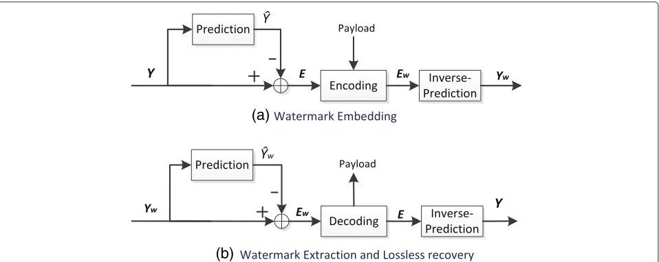
5 Encoder and decoder
The proposed reversible watermarking scheme, as illus-trated in Fig. 3, can be used for image or audio files. In this paper, we take some standard images for experi-mental testing. In the embedding, the maximal capacity (Pmax) of an image is first computed by using the proposed
reversible watermarking strategy,Pmax <= N. When an
actual payload sizeP(P<=Pmax)is given, the embedding
threshold T can be computed. For recovering the cover image, the information ofPandTis needed to be sent to the decoder in a way that the LSB values of the first 32 pre-diction errors are kept (as part of the payload) and then replaced by the parametersP(25 bits) andT(7 bits).
Referring to Sections 2 and 3, the embedding process of the proposed scheme is described as follows:
1. Referring to Section 3.4, predict the cover imageYto get the prediction errorsE;
2. Find the bad pixels in position by using an embedding testing operation. The embedding testing step is similar to that in [14, 15]. Each bad pixel consumes 25 bits of payload to indicate the embedding position; 3. Referring to Section 2.2, embed the data (includingP,
T, and the bad pixels in position) intoEto generate
Ew;
4. Reconstruct the marked imageYwfromEwby using the inverse prediction operation as described in Section 3.4, step 5).
In the decoder, the same prediction operations are per-formed on Yw to get Ew. Then, the information of P and T is extracted from the LSB values of the first 32 prediction errors. Furthermore, the hidden data and the
original prediction errorsEare extracted fromEw. Finally, the original imageY is completely recovered from E by using the inverse prediction operations.
6 Experimental testing and analysis
In this section, we adopt 24 gray-level versions of Kodak test images (http://r0k.us/graphics/kodak/index. html) and four standard benchmark images (baboon, bar-bara,f16, andlenain Fig. 4) as data set. Firstly, the perfor-mance of the noncausal predictor proposed in Section 3.4 is tested by comparing with other several typical predic-tors. This is followed by a performance comparison of the proposed watermarking scheme against three exist-ing state-of-the-art works [14, 15, 18]. All the algorithms were implemented in Matlab, and the experiments were performed by embedding and decoding randomly gener-ated binary bitstreams on image data set for reversible watermarking.
6.1 Comparison of typical predictors
The shape of the histogram of the predicted errors is often used to measure the performance of the embedding scheme. In general, distribution of the prediction errors obeys a Laplacian distribution. The shape of the distribu-tion is determined by the absolute mean and variance. If the mean is close to zero, the variance essentially deter-mines the shape of the histogram. The smaller variance value, the better performance can be achieved for the reversible watermarking scheme.
In the literature, the predictor proposed in [15] provides a satisfactory performance by dividing an image into two sets (like a chess board divided into black and white sets) to achieve noncausal prediction in a way that a pixel can be predicted with its four immediate pixels. This predic-tion method is suffering from a distorpredic-tion problem. That
Fig. 4Four standard benchmark images.aLena.bBaboon.cFishingboat.dF16
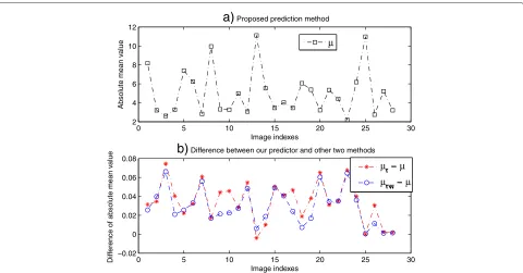
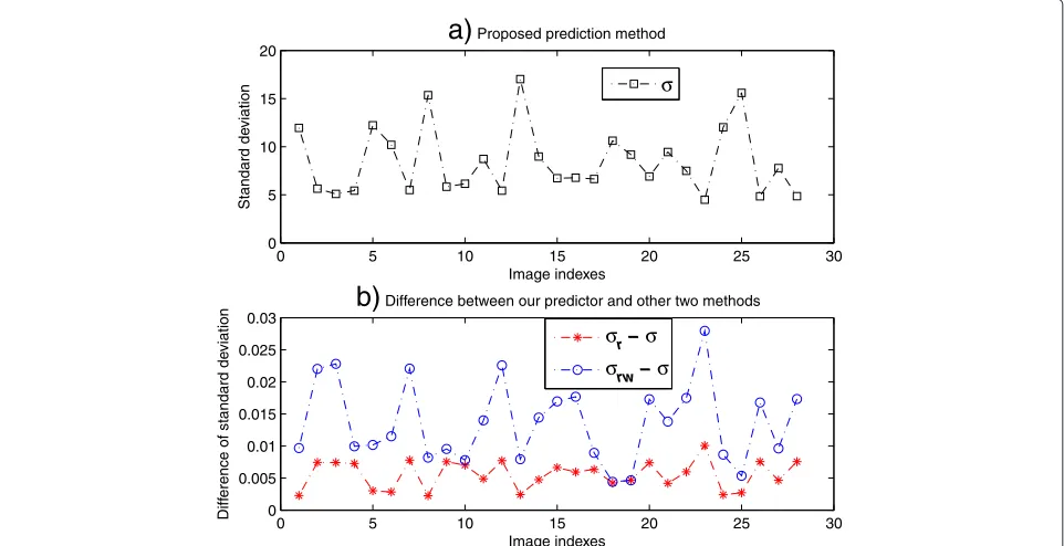
is, half of the pixels were predicted with modified pixels instead of the original ones. As shown in Section 3.4, the proposed prediction method can predict a pixel with its four immediate pixels, and all the pixels can be predicted completely with original pixels as context. As a result, the proposed prediction method has better prediction accu-racy. In order to better evaluate the effect of the round-ing and watermarkround-ing operations, we have computed the absolute mean values and the standard deviations of all the 28 test images which are predicted with the proposed predictor in this paper (denoted byμandσ), the proposed predictor with an integer rounding operation (μrandσr) and the prediction method in [15] (μrwandσrw).
Figure 5 shows the absolute mean values of all the 28 test images which are predicted with the proposed
method in this paper and the differences among these three predictors. We can see from Fig. 5a that the mean values are close to zero. In Fig. 5b, the differences (μr−μ) plotted with the “asterisk” line are often positive, indicat-ing the effect of the roundindicat-ing operation on the predicted values. The “circle” line plots the differences (μrw−μ) that are also positive, indicating the effect of prediction with the modified pixels on the mean values. Figure 6 shows the corresponding standard deviations (σ) and their dif-ferences, denoted by σr −σ and σrw − σ, respectively. We can see from the “asterisk” line in Fig. 6b that the difference values are always positive, indicating effect of the rounding operation and prediction with modified pix-els on the standard deviations. Figures 5 and 6 show that the prediction errors with the proposed predictor
0 5 10 15 20 25 30
2 4 6 8 10 12
Image indexes
Absolute mean v
alue
a)
Proposed prediction methodμ
0 5 10 15 20 25 30
−0.02 0 0.02 0.04 0.06 0.08
Image indexes
Diff
erence of absolute mean v
alue
b)
Difference between our predictor and other two methodsμr − μ μrw − μ
0 5 10 15 20 25 30 0
5 10 15 20
Image indexes
Standard de
viation
a)
Proposed prediction methodσ
0 5 10 15 20 25 30
0 0.005 0.01 0.015 0.02 0.025 0.03
Image indexes
Diff
erence of standard de
viation
b)
Difference between our predictor and other two methodsσr − σ σrw − σ
Fig. 6The standard deviations of the prediction errors and the differences of different prediction methods.aProposed prediction method.b Difference between our predictor and other two methods
has smaller mean value and the standard variances for an image.
Furthermore, Table 1 lists the absolute mean values and the standard deviations of four benchmark images pre-dicted with five different predictors (difference predictor used in [9, 10], integer MED predictor used in [14, 18], non-integer MED predictor [33], the prediction method in [15], and the proposed one in this paper). We can see from this table that the prediction method proposed in this paper can provide the smallest mean values and standard deviations.
6.2 Comparison with other recent algorithms
We implemented three typical algorithms: Thodi and Rodriguez’s IPE algorithm with histogram shifting and flag bits (P3) [14], Coltuc’s low distortion transform method on MED predictor [18], and the IPE-based double-embedding scheme [15] and the proposed scheme
with the NIPE technique and the new prediction method. The scheme, proposed by Thodi and Rodriguez, is the classical IPE embedding strategy which includes a MED predictor to output integer prediction errors for expan-sion embedding. Reversible watermarking using low dis-tortion transforms the same MED predictor proposed by Coltuc for the reduction of the embedding distortion by marking not only the current pixel but also its con-text [18]. In the literature, the double-embedding scheme proposed by Sachnev et al. has provided a satisfactory performance by dividing an image into two sets in a way that the pixels can be predicted in a noncausal way. Four standard benchmark images are adopted to report exper-imental results, as plotted in Fig. 7. Simulation results are similar for the other test images. We can see from Fig. 7 that the NIPE technique with the proposed noncausal pre-diction method performs better at all embedding rates. The detail is described as follows.
Table 1Performance comparison of five predictors
Predictors Lena Baboon Fishingboat F16
μ σ μ σ μ σ μ σ
Difference predictor [9, 10] 4.6724 7.8454 18.4130 27.6633 7.2441 11.1876 5.2971 11.9235
Integer MED predictor [14] 4.3407 6.9049 13.5220 19.6804 6.3836 9.3957 3.4273 6.2054
Non-integer MED predictor [33] 4.3060 6.7608 13.3652 19.2567 6.5863 9.7152 3.6089 6.6339
Sachnev’s predictor [15] 3.2063 4.8738 10.9786 15.6010 5.2220 7.7943 2.7578 4.8683
0 0.2 0.4 0.6 0.8 1
Fig. 7Comparison of capacity and fidelity against three typical algorithms [14, 15, 18]
The classical IPE embedding scheme, proposed by Thodi and Rodriguez [14], is a high-capacity reversible watermarking algorithm by developing PE embedding technique with MED predictor. We can see from Fig. 7 that the NIPE technique with the proposed noncausal predictor can provide higher embedding payload in com-parison with the IPE scheme. The basic reason is that the proposed noncausal predictor has higher prediction precision than the MED predictor used in [14].
Coltuc [18, 19] has also developed Thodi and Rodriguez’s work and has presented the results for the MED predictor. The basic idea of the approach is to embed the entire expanded difference not only into the current pixel but also its context. Then, the minimization of the square errors is considered to reduce the embed-ding distortion. When the parameterα is 0.25 (referred to [18], Eq. (4)), we can see from Fig. 7 that Coltuc’s embedding method has lower embedding distortion than the IPE for the same embedding rate. In [19], the embedding approach has been further generalized as a low distortion transform (LDT) for reversible water-marking. Comparing with the LDT technique with the MED predictor in [18], the proposed NIPE scheme can provide higher embedding payload or capacity for the same embedding distortion. The basic reason is that the proposed prediction strategy can better estimate the cur-rent pixel by incorporating data prediction not restricted to only causal pixels, as listed in Table 1.
Another important improvement on Thodi and Rodriguez’s work has been proposed by Sachnev et al. [15] by introducing a high-precision prediction strategy and sorting technique. Since a pixel can be estimated with its four immediate pixels, the IPE-based scheme can provide satisfactory performance in the literature. Figure 7 shows that the reversible watermarking approach proposed in this paper has lower embedding distortion at all embedding rates than Sachnev et al.’s double embed-ding scheme. The reason is that the predictor used for NIPE can predict pixels with four original immediate pixels when one used in [15] predicted half of pixels with modified pixels as context.
7 Conclusions
pixels. With the proposed NIPE and predictor, the embed-ding distortion is smaller than that in [15] at all embedembed-ding rates. Experimental results have shown that the predic-tor designed in this paper can provide the best perfor-mance than several existing typical prediction methods. In comparison with other typical reversible watermarking algorithms, the proposed scheme (combining the NIPE technique and new prediction method) performs better.
Endnotes
1In the IPE, the prediction errors should be rounded to integer value. This rounding operation brings a
constraint on a predictor’s performance.
2In the literature [15, 26], noncausal predictive methods have been used for the IPE by using multi-passes prediction for multi-layers embedding. Since part of the pixels were predicted by using the watermarked pixels instead of the original ones, some distortion has been introduced.
Competing interests
The authors declare that they have no competing interests.
Acknowledgements
This work was supported by NSFC (No. 61272414). The authors would like to thank the reviewers’ valuable comments.
Received: 11 October 2014 Accepted: 16 May 2015
References
1. W Bender, D Gruhl, N Morimoto, A Lu, Techniques for data hiding. IBM Syst. J.35(3), 313–336 (1996)
2. B Macq, inProc. the European Signal Processing Conf,. Lossless multiresolution transform for image authenticating watermarking (Tampere, Finland, 2000)
3. C De Vleeschouwer, JE Delaigle, B Macq, Circular interpretation of bijective transformations in lossless watermarking for media asset management. IEEE Trans. Multimedia.5(1), 97–105 (2003) 4. S Lee, CD Yoo, T Kalker, Reversible image watermarking based on
integer-to-integer wavelet transform. IEEE Trans. Inf. Forensics Secur. 2(3), 321–330 (2010)
5. J Fridrich, M Goljan, R Du, inProc. SPIE Photonics West, Security and Watermarking of Multimedia Contents III. Invertible authentication, vol. 3971 (San Jose, 2001), pp. 197–208
6. J Fridrich, M Goljan, R Du, Lossless data embeddinga¸ł paradigm in digital watermarking. EURASIP J. Appl. Signal Process.2, 185–196 (2002) 7. AACM Kalker, FMJ Willems, inProc. 14th Int. Conf. Digital Signal Processing.
Capacity bounds and constructions for reversible data-hiding, vol. 1 (Santorini, 2002), pp. 71–76
8. MU Celik, G Sharma, AM Tekalp, E Saber, Lossless generalized-LSB data embedding. IEEE Trans. Image Process.14(2), 253–266 (2005) 9. J Tian, Reversible data embedding using a difference expansion. IEEE
Trans. Circuits Syst. Video Technol.13(8), 890–896 (2003)
10. AM Alattar, Reversible watermark using the difference expansion of a generalized integer transform. IEEE Trans. Image Process.13(8), 1147–1156 (2004)
11. L Kamstra, H Heijmans, Reversible data embedding into images using wavelet techniques and sorting. IEEE Trans. Image Process.14(12), 2082–2090 (2005)
12. X Wang, C Shao, X Xu, X Niu, Reversible data-hiding scheme for 2-D vector maps based on difference expansion. IEEE Trans. Inf. Forensics Secur.2, 311–319 (2007)
13. Y Hu, H-K Lee, J Li, DE-based reversible data hiding with improved overflow location map. IEEE Trans. Circuits Syst. Video Technol. 19(2), 250–260 (2009)
14. DM Thodi, JJ Rodriguez, Expansion embedding techniques for reversible watermarking. IEEE Trans. Image Process.15, 721–729 (2007)
15. V Sachnev, HJ Kim, J Nam, S Suresh, Y Shi, Reversible watermarking algorithm using sorting and prediction. IEEE Trans. Circuits Syst. Video Technol.19(7), 989–999 (2009)
16. H-W Tseng, C-P Hsieh, Prediction-based reversible data hiding. Inf. Sci. 179, 246–2469 (2009)
17. X Li, B Yang, T Zeng, Efficient reversible watermarking based on adaptive prediction-error expansion and pixel selection. IEEE Trans. Image Process. 20(12), 3524–3533 (2011)
18. D Coltuc, Improved embedding for prediction-based reversible watermarking. IEEE Trans. Inf. Forensics Secur.6(3), 873–882 (2011) 19. D Coltuc, Low distortion transform for reversible watermarking. IEEE
Trans. Image Process.21(1), 412–417 (2012)
20. Veen van der M, F Bruekers, A van Leest, S Cavin, inProc. SPIE Photonics West, Electronic Imaging 2003, Security and Watermarking of Multimedia Contents V. High-capacity reversible watermarking for audio, vol. 5020 (San Jose, California, 2003), pp. 1–11
21. B Bradley, AM Alattar, inProc. SPIE Photonics West, Electronic Imaging 2005, Security and Watermarking of Multimedia Contents VII. High-capacity, invertible, data-hiding algorithm for digital audio, vol. 5681 (San Jose, California, 2005), pp. 789–800
22. D Yan, R Wang, inInternational Conference on Intelligent Information Hiding and Multimedia Signal Processing. Reversible data hiding for audio based on prediction error expansion (Harbin, 2008), pp. 249–252
23. A Van Leest, M Van der Veen, F Bruekers, inProc. IEEE Conf. Image Processing. Reversible image watermarking, vol. 3 (Barcelona, 2003), pp. 731–734
24. Z Ni, Y Shi, N Ansari, S Wei, inProc. IEEE Int. Symp. Circuits and Systems. Reversible data hiding, vol. 2 (Bangkok, 2003), pp. 912–915
25. M Chen, Z Chen, X Zeng, Z Xiong, inProc. 11th ACM Workshop Multimedia and Security. Reversible data hiding using additive prediction-error expansion (Princeton, 2009), pp. 19–24
26. L Luo, Z Chen, M Chen, X Zeng, Z Xiong, Reversible image watermarking using interpolation technique. IEEE Trans. Inf. Forensics Security. 5(1), 187–193 (2010)
27. Anil K Jain,Fundamentals of digital image processing. (Prentice, Hall, Englewood Cliffs, NJ, 1989)
28. A Asif, JMF Moura, Image codec by noncausal prediction, residual mean removal, and cascaded vector quantization. IEEE Trans. Circuits Syst. Video Technol.6(1), 42–55 (1996)
29. N Balram, JMF Moura, Noncausal predictive image codec. IEEE Trans. Image Process.5(8), 1229–1242 (1996)
30. M Weinberger, G Seroussi, Sapiro G, The LOCO-I lossless image compression algorithm: principles and standardization into JPEG-LS. IEEE Trans. Image Process.9(8), 1309–1324 (2000)
31. WR Gardner, BD Rao, Non-causal linear prediction of voiced speech. IEEE Asilomar Conference on Signals, Systems and Computers, (Pacific Grove, CA, Oct. 1992), pp. 1100–1104
32. Wu X, Memon N, Context-based, adaptive, lossless image coding. IEEE Trans. Commun.45(4), 437–444 (1997)
33. S Martucci, inProc. IEEE Int. Symp. Circuits and Systems. Reversible compression of HDTV images using median adaptive prediction and arithmetic coding (New Orleans, 1990), pp. 1310–1313
![Fig. 7 Comparison of capacity and fidelity against three typical algorithms [14, 15, 18]](https://thumb-us.123doks.com/thumbv2/123dok_us/891677.1107283/11.595.58.541.87.351/fig-comparison-capacity-fidelity-typical-algorithms.webp)
