R E S E A R C H
Open Access
Significance-aware filtering for nonlinear
acoustic echo cancellation
Christian Hofmann
*, Christian Huemmer, Michael Guenther and Walter Kellermann
Abstract
This article summarizes and extends the recently proposed concept of Significance-Aware (SA) filtering for nonlinear acoustic echo cancellation. The core idea of SA filtering is to decompose the estimation of the nonlinear echo path into beneficially interacting subsystems, each of which can be adapted with high computational efficiency. The previously proposed SA Hammerstein Group Models (SA-HGMs) decompose the nonlinear acoustic echo path into a direct-path part, modeled by a Hammerstein Group Model (HGM) and a complementary part, modeled by a very efficient Hammerstein model. In this article, we furthermore propose a novel Equalization-based SA (ESA) structure, where the echo path is equalized by a linear filter to allow for an estimation of the loudspeaker nonlinearities by very small and efficient models. Additionally, we provide a novel in-depth analysis of the computational complexity of the previously proposed SA and the novel ESA filters and compare both SA filtering approaches to each other, to adaptive HGMs, and to linear filters, where fast partitioned-block frequency-domain realizations of the competing filter structures are considered. Finally, the echo reduction performance of the proposed SA filtering approaches is verified using real recordings from a commercially available smartphone. Beyond the scope of previous publications on SA-HGMs, the ability of the SA filters to generalize for double-talk situations is explicitly considered as well. The low complexity as well as the good echo reduction performance of both SA filters illustrate the potential of SA filtering in practice.
Keywords: Significance-aware, Equalization-based significance-aware, Efficiency, Nonlinear acoustic echo cancellation, Hammerstein group model, Hammerstein model
1 Introduction
Since the first adaptive linear echo canceler for network echoes in telephone lines [1], linear echo cancellation has evolved to a key ingredient of almost any full-duplex speech communication system. This has resulted in a mul-titude of approaches to efficiently model, parametrize, and estimate even complex linear systems, such as the acoustic echo paths in hands-free wideband telecommu-nication scenarios [2]. With increasingly common nonlin-ear distortions produced by miniaturized amplifiers and loudspeakers in modern portable devices, dedicated non-linear echo path models have emerged as an important topic of research and motivated sophisticated approaches for nonlinear Acoustic Echo Cancellation (AEC) based on Volterra filters [3–5], artificial neural networks [6, 7], Functional Link Adaptive Filters (FLAFs) [8, 9], or kernel
*Correspondence: [email protected]
1Multimedia Communications and Signal Processing,
Friedrich-Alexander-Universität Erlangen-Nürnberg (FAU), Cauerstraße 7, Erlangen, Germany
methods [10, 11]. A very simple, yet effective model for nonlinear acoustic echo paths is the cascade of a memo-ryless preprocessor (modeling loudspeaker signal distor-tions) and a subsequent linear system (modeling sound propagation through air) [12]. Due to its simplicity, this so-called Hammerstein Model (HM) has been frequently employed [13–22] and will also be used in this contribu-tion. So will be a group of B parallel HMs, referred to as Hammerstein Group Model (HGM) in the following. The recently proposed efficient Significance-Aware HGM (SA-HGM) [20] combines the advantages of HMs and HGMs and was extended to an efficient partitioned-block frequency-domain realization in [22].
Beyond previous work, this article introduces a novel variant of the Significance-Aware (SA) filtering concept denoted as Equalization-based SA (ESA) filtering which complements the existing efficient frequency-domain realization in [22]. Thereby, highly efficient SA filters can be derived for higher-order nonlinear systems—even without block partitioning. Furthermore, a novel in-depth
analysis of the computational complexity of the previously proposed SA filtering concepts is provided and contrasted with the computational complexity of the novel ESA filter-ing concept, adaptive HGMs, and conventional adaptive linear filters. Beyond previous investigations [22], this article also assesses the ability of the considered echo path models to generalize for double-talk situations, in which the models cannot be adapted to the current input sig-nal. The performance in such situations reflects how well the estimated system models the physical system to be identified.
The remainder of this paper is structured as fol-lows: after introducing the notation in Section 2, fre-quently used echo path models and their adaptation are reviewed in Sections 3.1 and 3.2, respectively. After-wards, the recently proposed Partitioned-Block SA-HGM (PBSA-HGM) is summarized in Section 4.1, before intro-ducing the novel ESA filtering concept in Section 4.2, which results in an Equalization-based Significance-Aware HM (ESA-HM). Then, the computational com-plexity of the SA filters (PBSA-HGM and ESA-HM) is analyzed and compared to the complexity for adapting a linear model and an HGM in Section 5.1. An experimen-tal verification of the efficacy of the novel ESA-HM in comparison to other approaches in terms of echo reduc-tion performance is given in Secreduc-tion 5.2. Finally, the manuscript is complemented by a summary of the main results in Section 6.
2 Notation
Throughout this article, vectors will be typeset in bold-face lowercase letters, e.g.,a, and matrices in uppercase boldface, e.g.,A. The complex conjugate, transposed, and
Hermitian-transposed of a vector a (column vector by
default) will be written as a∗, aT, and aH, respectively. Besides,AB,AB, and|A|2denote element-wise multi-plication (Hadamard product), element-wise division, and element-wise magnitude-squaring of matrices or vectors of the same size, respectively. Furthermore,a,bstands for the scalar productaHb. Special matrices are theM×M identity matrixIM, theM×Mall-zero matrix0M, and the windowing matrices
W01=
0M 0M 0M IM
and W10=
IM 0M 0M 0M
, (1)
setting the first or second half of a length-2M vector to zero, respectively. Furthermore,F andFHdenote the Nth-order Discrete Fourier Transform (DFT) matrix and its inverse, respectively. Besides, a(k) ∗b(k) anda(k) b(k) denote linear and cyclic convolution between time seriesa(k)andb(k), respectively, wherekis the discrete-time sample index. Analogously to vectors,a(k),b(k) =
∞
k=−∞a(k)b∗(k)denotes the scalar product between the time seriesa(k)andb(k). For a real-valued scalara,a
refers to the smallest integer number larger than or equal toa, also known as ceiling function.
3 Fundamentals of linear and nonlinear acoustic echo cancellation
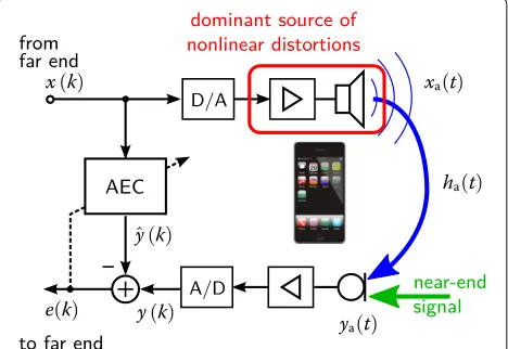
The acoustic echo path of a full-duplex communication system can be described as illustrated in Fig. 1.
Therein, the discrete-time loudspeaker signal x(k), where kis the sample index, is interpolated by the D/A converter, amplified, and played-back via a loudspeaker, yielding the analog loudspeaker signalxa(t), wheretis the continuous time variable. The subsequent propagation of the sound waves through the medium air to the micro-phone can be modeled very accurately by a linear sys-tem with impulse responseha(t). These acoustic echoes (far-end components) superimpose with local speakers and interferences (near-end components), evoking the continuous-time microphone signalya(t)and its sampled, discrete-time representation y(k). In order to provide good estimates of local (near-end) speakers, two technolo-gies are typically employed: an AEC unit for removing the far-end signal components fromy(k)and a postfilter suppressing residual echoes and near-end interferences [23–32].
In this work, we will not address the latter but focus on the AEC unit, which provides an echo estimateyˆ(k) by identifying the acoustic echo path adaptively. The AEC error signal
e(k)=y(k)− ˆy(k)
is an estimate for the near-end signal, even during double-talk periods, where both far-end and near-end compo-nents are present. In periods of vanishing near-end signal (single-talk periods),e(k)can be used for refining the echo path estimate. Thus, the AEC unit typically requires a double-talk detection [33–38]. As double-talk detection
is out of the scope of this article, we will assume this to be handled separately, such that the microphone signal during time intervals used for echo path estimation only consists of far-end signal components (acoustic echoes). Furthermore, the AEC unit requires the choice of a suit-able echo path model and of an adaptation strategy. This will be addressed in Sections 3.1 and 3.2, respectively.
3.1 From linear to nonlinear echo path models
This section contains a brief overview of frequently employed echo path models. Strategies for estimating the model parameters (i.e., filter coefficients) will be described in Section 3.2.
3.1.1 Linear models
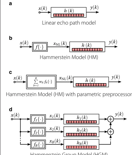
The most simple, yet frequently used echo path model is the linear model, depicted in Fig. 2a.
Therein, the Loudspeaker-Enclosure-Microphone Sys-tem (LEMS) is modeled by a linear FIR filter with the input/output relation
y(k)=x(k)∗h(k), (2)
whereh(k) is the discrete-time impulse response of the LEMS. Such models are most suitable for high-quality audio equipment. On the other hand, energy-efficient and miniaturized portable devices operating at the limit of their capabilities (such as portable navigation devices or
Fig. 2 a–dFrequently used echo path models for AEC, where each of the red blocks represents a fixed number of coefficients of a linear Finite Impulse Response (FIR) filter
smartphones in hands-free mode) lead to nonlinear dis-tortions in the played-back signal [12] (see red box in Fig. 1), which render linear echo path models insufficient.
3.1.2 Hammerstein models
Due to the cascaded nature of the acoustic echo path between x(k) and y(k) (first nonlinear playback equip-ment, then linear transmission through air), a very simple, yet effective nonlinear echo path model is given by the cascade of a memoryless nonlinearity (memoryless pre-processor) with a subsequent linear system [12–22]. Such a structure is depicted in Fig. 2b and is referred to as HM or nonlinear-linear cascade in the literature [39–43]. This corresponds to the input/output relation
y(k)=h(k)∗xNL(k)
=h(k)∗f{x(k)}. (3)
In AEC, the memoryless preprocessor xNL(k) =
f{x(k)}typically has to model a saturation introduced by the amplifier and the loudspeaker. To this end, f{x(k)} can be chosen from a simple hard limiter to a parametric preprocessor [14]
xNL(k)= B
b=1
wbfb{x(k)} (4)
with nonlinearity basis functions fb{·} and preproces-sor weights (parameters) wb, which corresponds to the block diagram in Fig. 2c. Considering aBth-order poly-nomial preprocessor, intermodulation products up to the
orderBmay be modeled. Examples for such polynomial
preprocessors can be found in [13, 14].
3.1.3 Hammerstein group models
A more complex and more general class of models will be referred to as HGMs. They consist, as depicted in Fig. 2d, of a group ofBparallel HMs and have individual impulse responseshb(k)(referred to as kernels) for each branch b=1,. . .,Bafter the branch’s nonlinearity basis function fb{·}. This corresponds to the input/output relation
y(k)= B
b=1
hb(k)∗f b{x(k)}
xb(k)
, (5)
where xb(k) will be referred to as branch signals in the following.
larger expanded vector, which is mapped to an echo esti-mate by linear combination (covers both convolution and summation in (5)). However, with focus on the appli-cability of fast convolution methods in this article, the formulation according to a group of parallel Hammerstein systems is advantageous.
Furthermore, note that the special case of an HGM where allhb(k) =wbhbref(k)∀b =1,. . .,Bare scaled ver-sions of a reference impulse responsehbref(k) in branch
brefcan be expressed as an HM. One possible HM
rep-resentation of such an HGM has the reference impulse response h(k) = hbref(k) and a parametric preproces-sor according to (4) with the HGM’s nonlinearity basis functionsfb{·}and preprocessor weights
wb=
This correspondence will be essential for the SA filters in Section 4, where bref = 1 (implyingw1 = 1) will be considered by default.
3.1.4 Models with dynamic nonlinearities
A further generalization of HGMs are models, where the nonlinearity basis functions are nonlinear functions fb{x(k)}depending on a vectorx(k), which is formed from samples of the input signal x(k). The most prominent example for such filters are the so-called Volterra filters [3–5, 40, 46–48], for whichfb{x(k)}computes time-lagged products of samples ofx(k)(different elements ofx(k))1. Note that power filters [44, 45] (having a memoryless non-linearity) represent the special case of the Volterra filters where only the main diagonal of each Volterra kernel is populated with non-zero coefficients, corresponding to the respective kernels of the power filter. Volterra filters can be seen as a multidimensional Taylor series expansion of the function x(k) → y(k). Alternatively, the mono-mial basis functions of Volterra filters have also been replaced by Legendre polynomials [49, 50] or Fourier basis functions (sinusoids) [51]. Note that for the Fourier-basis nonlinear filters, the feed-forward structure has also been complemented by a feedback path, leading to bounded-input/bounded-output (BIBO)-stable recursive nonlinear filters [52].
Although the SA filters described in Section 4 will employ only HGMs and memoryless preprocessors, it is worth noticing that the SA filtering concept can also be applied to dynamic nonlinearitiesfb{x(k)}, involving, e.g., Volterra filters instead of HGMs.
3.2 Adaptation strategies
Adaptation of nonlinear models can be performed on dif-ferent levels. On a basic level, parameters like filter coef-ficients of a model with a given structure are identified.
To this end, the parameters may be modeled as deter-ministic parameters, resulting in, e.g., Least-Mean-Square (LMS) algorithms [53] for adaptation, or as probabilis-tic parameters, leading to Kalman filter-like algorithms [15, 19, 21, 54]. On a higher level, the model structure (e.g., filter lengths of linear subsystems or numbers of diagonals of Volterra kernels) can be estimated via self-configuring evolutionary algorithms [5, 55–57]. In this article, the term “adaptation” will refer to the iterative estimation of filter coefficients modeled as deterministic parameters of a model with fixed structure.
In this section, the adaptation of the linear subsystems of the models described in Section 3.1 will be discussed. As all these models can be expressed as special cases of a parallel structure like an HGM, the adaptation will be described for an HGM. Then, the adaptation schemes for all other models can be derived as special cases of the HGM case. In particular, two common approaches for filter adaptation will be revisited: the direct adaptation of the impulse responses in the time domain by a Normal-ized Least-Mean-Square (NLMS) algorithm and the adap-tation of partitioned versions of the impulse responses in the frequency domain, which allows a smooth trade-off between computational efficiency and algorithmic delay (latency) of the digital signal processing system.
3.2.1 Time-domain adaptive filtering
A straightforward identification of the linear filters of an HGM is possible by iteratively minimizing a quadratic cost function derived from the error signale(k). Most com-mon algorithms are LMS-, affine projection-, or Recursive Least-Squares (RLS)-type algorithms [53]. Due to its com-putational efficiency, the adaptation of an HGM by an NLMS algorithm, which aims at minimizing the Mean Squared Error (MSE) in a gradient-descent manner, will be considered. The following description is independent of the actual choice of the nonlinearity basis functionsfb{·}, as long asfb{·}are time-invariant (Legendre polynomials will be employed for the evaluations in Section 5).
An adaptive HGM with such time-invariant nonlinear-ity basis functionsfb{·}first computes the branch signals
xb(k)=fb{x(k)} (7)
and afterwards the echo estimate
ˆ the impulse response in branchband has been obtained at time indexk−1. Then, the error signal
has to be computed, before performing for each branchb and filter taplan update according to
ˆ
hb,l(k)= ˆhb,l(k−1)+μb· e(k) Exb(k)+δ
xb(k−l), (10)
where 0 < μb < 1 are branch-specific adaptation step-sizes, Exb(k) =
L−1
l=0 |xb(k−l)|2are the branch signal energies, and δ is a regularization constant for numeri-cal stability2. An efficient implementation (as assumed for the complexity analysis in Section 5.1) decomposes (10) by determining branch powers
Pxb(k)=(xb(k))
2 (11)
to compute the branch energies
Exb(k)=Exb(k−1)+Pxb(k)−Pxb(k−L), (12)
and finally updates the filter coefficients according to
ˆ
hb,l(k)= ˆhb,l(k−1)+enorm,b(k)xb(k−l). (14)
This allows to adaptively identify the individual branches of HGMs but also covers the identification of single HMs and linear models as special cases.
3.2.2 Partitioned-block frequency-domain adaptive filtering
Partitioned-block convolution: A linear convolution can be realized despite large filter lengthsL with a low input/output delay efficiently by block-based processing methods like Partitioned-Block Frequency-Domain Fil-tering (PBFDF) [56, 58–60], also known as multidelay convolution [61]. In the following, only a uniform parti-tioning with frame shiftMand frame sizeN=2Mwill be considered.
In this case, the input signalx(k), the impulse response h(k), and the output signal y(k) are partitioned into
respectively, where κ is the frame index for block pro-cessing andpis the index of the impulse response parti-tion. After a DFT, represented by the DFT matrixF, the transformed versions of the signal vectors and impulse response partitions are referred to as
x(κ)=Fx(κ) (18)
h(p)=Fh(p). (19)
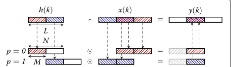
As illustrated in Fig. 3 forP= 2 partitions, performing fast DFT-domain convolution between each pair ofh(p)
Fig. 3Example for partitioned block convolution usingP= 2 blocks for partitioning the Impulse Response (IR)h(k): the summation during convolution is split intoP= 2 partial sums of lengthM. Each partition ofh(k) produces a sequence ofMsamples of its contribution to the convolutive product in an overlap-save manner in the DFT domain, where the block length isN= 2M. Summing up the second half of these partial results (free from cyclic convolution artifacts) yields a block ofMoutput samples (see [22])
andx(κ−p)and summing up the respective partial results yields
response partitions and where the windowing matrixW01 according to (1) suppresses additionally computed sam-ples iny◦(κ), which result from the previous frame and may contain cyclic convolution artifacts.
Note that such a PBFDF scheme is computationally effi-cient because each input signal frame’s DFT has to be computed only once.
Partitioned-block frequency-domain adaptive filtering (PBFDAF): In the following, partitioned-block convolu-tion will be utilized during the adaptaconvolu-tion of an HGM with DFT-domain filter estimateshˆ(bp)(κ) for partitionp
in branch b at time frame κ. As for the time-domain
xb(κ)=
which are then transformed into the DFT domain accord-ing to
xb(κ)=Fxb(κ). (22)
This allows the computation of the DFT-domain error signal vector
is the intermediate DFT-domain microphone signal esti-mate with cyclic convolution artifacts of the partitioned-block convolution andyˆ(κ)is the final time-domain
esti-mate containingMzeros and theMmost recent samples
of ˆy(k). Similar to the time-domain adaptation, branch signal Power Spectral Density (PSD) vectors
sxb(κ)=γEsxb(κ−1)+(1−γE)xb(κ)2 (25) are calculated in the DFT domain by recursively smooth-ing the element-wise squared magnitudes xb(κ)2 with 0 ≤ γE < 1. In the following,γE = 0.9 will be employed as default. Based onsx
b(κ), normalized branch signals are
computed according to
before performing the actual filter update according to
˜
h(bp)(κ)= ˆh(bp)(κ−1)+xnorm,b(κ−p)e(κ). (27)
Additionally, the temporal support of the filters can be limited explicitly to the partition lengthM
ˆ
This is equivalent to the classical formulation of the so-called constrained update, where the constraint (zeros in time domain) is imposed on the update (see [61]). Yet, the computation ofhˆ(bp)(κ) as a byproduct of the filter con-straint in (28) will be beneficial for the SA filtering later on.
As for time-domain adaptive filtering, the algorithm for adapting an HGM in the partitioned-block frequency domain covers the adaptation of an HM (an HGM with B = 1 andf1{x(k)} = f{x(k)}) and a linear model (an
HGM withB = 1 and x1(k) = f1{x(k)} = f{x(k)} = x(k)). Furthermore, the non-partitioned FNLMS algo-rithm, derived in many textbooks, e.g., [53, 62], results from the aforementioned partitioned-block description for P = 1 with sufficiently large N = 2L. Adapting a model with the block partitioning will be referred to as Partitioned-Block Frequency-domain Normalized Least Mean Squares (PB-FNLMS) algorithm.
4 Significance-aware filtering
Significance-aware (SA) filtering is a generalized system identification concept which exploits prior knowledge about the physical system to be identified by decomposing the adaptive model in a divide-and-conquer manner into beneficially interacting subsystems.
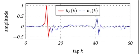
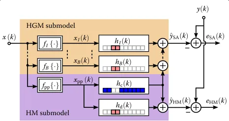
In particular, the originally proposed SA-HGM [20] per-forms a temporal decomposition of the acoustic echo path, as depicted in Fig. 4 for a linear model, into a region describing the direct-path wavefront and a complemen-tary region.
This decomposition is then employed, as depicted in Fig. 5, to model the short direct-path region (carrying a significant amount of energy) by an HGM and to model the large complementary region by a computationally effi-cient HM. Apart from the decomposition into subsystems, the interaction between the subsystems is a key feature of SA filtering as well. In particular, the HM subsystem’s nonlinear preprocessor has the form
xpp(k)=fpp{x(k)} =
and combines the branch signals xb(k) with frame-wise updated weights wˆb(κ). These weights wˆb(κ) are esti-mated from the kernels of the HGM subsystem (will be explained in Section 4.1.3). Thereby, a nonlinear model estimated from the direct path is extrapolated to the entire acoustic echo path.
These two features, the decomposition and the pre-processor coefficient estimation via an HGM, are key components of both the recently proposed PBSA-HGM [22], revisited in Section 4.1, and the novel alternative SA
Fig. 5SA-HGM for efficient nonlinear system identification: the temporal support modeled by the filters is color-coded by thesquares
below the IR symbolsh∗.White squaresindicate unmodeled temporal support andredandblue squaresrepresent modeled support corresponding to the direct path and the complementary region, respectively. Typically,ˆySA(k) is employed as final echo estimate
filtering structure, which will be denoted by ESA filtering and will be introduced in Section 4.2.
4.1 Significance-aware Hammerstein group models SA-HGMs are efficient because the potentially compu-tationally expensive HGM only has to model a small temporal support of the acoustic echo path. To realize this concept while exploiting the benefit of fast frequency-domain convolution, a partitioned-block variant of the SA-HGMs, denoted as PBSA-HGM, has recently been
introduced in [22]3. This PBSA-HGM will be briefly
reviewed in the following. Employing the uniform par-titioning according to Section 3.2.2 leads to an adaptive HM with DFT-domain partition estimateshˆ(p)(κ)for
par-titions p = 0,. . .,P − 1 and an adaptive HGM with
DFT-domain estimateshˆ(bpd)(κ)for branchesb=1,. . .,B but just a single partition with index pd. This partition with index pd should capture the direct path and thus a significant portion of the energy transmitted from the loudspeaker to the microphone. Note thathˆ(pd)(κ) mod-elshd(k)in Fig. 5 andhˆ(p)(κ)∀p=pdjointly modelhc(k) in Fig. 5. In the following, the estimation ofhˆ(p)(κ) (cov-ering bothhd(k)andhc(k)of Fig. 5) andhˆ(bpd)(κ)will be described in Sections 4.1.1 and 4.1.2, respectively, and the estimation of the HM’s preprocessor coefficients wˆb(κ) based onhˆ(bpd)(κ)will be explained in Section 4.1.3.
4.1.1 Estimation of the RIR of the HM submodel
In the following, the identification of the HM subsys-tem’s impulse response partitions will be described. For this purpose, the preprocessed loudspeaker signal can be expressed in vector notation as
xpp(κ)=
where xb(κ) are the branch signal vectors of the HGM submodel. The HM submodel with DFT-domain partition estimateshˆ(p)(κ)yields, analogously to (23), an echo
sig-The HM submodel’s DFT-domain error vector can then be computed via
eHM(κ)=Fy(κ)− ˆyHM(κ). (32)
Iteratively minimizing the two-norm of eHM(κ) in a gradient-descent manner by an FNLMS algorithm leads to the update rule
wherexnorm,pp(κ−p)is the normalized DFT-domain sig-nal vector computed asig-nalogously to (26) from the prepro-cessed inputxpp(κ).
4.1.2 Estimating the HGM submodel
The HGM submodel alone provides an echo estimate
ˆ
which is combined with the complementary-region par-titions’ echo estimate of the HM submodel according to
ˆ
Minimizing the two-norm of the error signal vector
eSA(κ)=Fy(κ)− ˆySA(κ) (36)
by an FNLMS algorithm leads to the update rule
ˆ
response partitions will become obvious in the following section.
4.1.3 Estimating the preprocessor of the HM
Finally, the HM’s preprocessor coefficients can be recom-puted employing the HGM. To avoid overhead due to complex-valued arithmetic, a direct use of the time-domain kernelshˆ(pd)
b (κ)(obtained as a byproduct of (37)) is possible to compute instantaneous least squares esti-mates for the preprocessor weights [20] according to
˜
A subsequent temporal smoothing of these estimates leads to the final preprocessor coefficients
ˆ
wb(κ+1)=γwwˆb(κ)+(1−γw)w˜b(κ), (40)
where 0 ≤ γw < 1. In the following, γw = 0.95 will be employed per default. Note thatwˆ1(κ) =1∀κand there-fore does not need to be computed at all. As in [20, 22], the first branch (b = 1) will be assumed to be linear (f1{x(t)} = x(t)), such that an entirely linear echo path model results from a preprocessor withwˆb(κ)=0 ∀b>1. By the method described in Section 4.1 and its subsec-tions, the estimation of the nonlinear system has been split into two beneficially interacting subproblems (HM and HGM adaptation). The beneficial interaction is achieved by the preprocessor coefficient refinement based on the HGM and by the extension of the temporal support of the HGM employing partitions of the HM. An in-depth evaluation of the computational complexity of such a PBSA-HGM will be given in Section 5.1.
4.2 Equalization-based significance-aware Hammerstein models
Previous applications of the SA concept [20–22] split the echo path model along the time axis (using knowledge about a dominating direct-path component), to allow for an efficient estimation of nonlinear parameters (see also Section 4.1). This corresponded to a parallel decomposi-tion of the acoustic echo path (seehc(k)andhd(k)of the HM submodel block in Fig. 5, wherefpp{·}can be shifted in the parallel branches ofhc(k)andhd(k)as well).
In this section, we propose a novel realization of the SA filtering concept. This realization employs a serial decom-position (a cascade) of the echo path into a nonlinear loudspeaker and a subsequent linear RIR, in order to esti-mate the nonlinear parameters of an HM (which is used
as actual echo path model). The resulting ESA-HM struc-ture is depicted in Fig. 6. Therein, the topmost branch contains the actual echo path, which is assumed to have Hammerstein structure. Below, there are three colored blocks comprising the novel structure denoted as ESA-HM. While blockαcomputes the actual echo estimate for
AEC by an HM, and blocks β andγ facilitate the
esti-mation of the nonlinear preprocessorfpp{·}of the HM in blockα. In the following, the ESA-HM will be explained
in a bottom-up manner, starting with block γ and
end-ing withα. To avoid redundancy, the employed adaptive filtering algorithms, all of which have been described in previous sections, are not entirely re-written for the particular filters to be estimated in this section but are referenced instead.
4.2.1 Equalization of the RIR (blockγ)
In block γ (Fig. 6), the ESA-HM directly exploits the
cascaded nature of the nonlinear echo path (memory-less nonlinearity f{·}, followed by an impulse response h(k)): the IRh(k)is equalized by an adaptive linear filter
of the delayed nonlinearly distorted loudspeaker signal xNL(k−L). The linear equalizerhˆeq,l(k)is identified by a PB-FNLMS algorithm (see Section 3.2.2) using the error signal
eeq(k)=x(k−L)− ˆxNL(k−L). (42)
On the one hand, (41) suggests thatxˆNL(k−L)is an esti-mate forx(k−L), obtained via linear filtering ofy(k). On the other hand, the linear equalizerhˆeq,l(k)cannot equal-ize the nonlinear components of the LEMS, such that the nonlinear distortion remains in the equalizer output and
ˆ
xNL(k−L)according to (41) can be seen as an estimate for the nonlinearly distorted signalxNL(k−L). Thus, while the inability of impulse responses to model nonlinear sys-tems hampers the performance of the AEC system in the first place, this inability is exploited here to estimate an otherwise inaccessible intermediate signal to guide the estimation of the nonlinear components (described in the next paragraphs). Furthermore, the equalization is only as complex as a single linear AEC system (assuming identical filter lengths).
4.2.2 Estimating the nonlinearity (blockβ)
Fig. 6Proposed novel ESA-HM for efficient nonlinear system identification: estimating an equalizing RIRhˆeq,l(k) to obtain an estimateˆxNL(k) of the
nonlinearly distorted loudspeaker signal (blockγ) allows to assess the nonlinear distortions by a very short HGM (blockβ), which in turn is used to estimate the preprocessor of the HM modeling the acoustic echo path (blockα)
in block γ (Fig. 6), such that xˆNL(k − L) is time-aligned with x(k − L). Thus, the nonlinear mapping between the discrete-time loudspeaker signal x(k − L) and the estimate of the nonlinear loudspeaker sig-nal xˆNL(k − L) can be modeled by an adaptive time-domain HGM with branch kernels hˆb(k) with a very
small temporal support of LSA taps (e.g., LSA = 3).
This corresponds to the input/output relation
ˆˆ
xNL(k−L)= B
b=1 LSA−1
l=0
x(k−L−l)· ˆhb,l(k−1). (43)
The adaptation ofhˆb,l(k)is performed by a time-domain NLMS algorithm (see Section 3.2.1) operating on the error signal
eeq,HGM(k)= ˆxNL(k−L)− ˆˆxNL(k−L). (44)
Due to the small number of modeled tapsLSA, such a time-domain algorithm is computationally inexpensive.
4.2.3 Estimating the preprocessor of the HM (between blocksβandα)
Analogously to the previously proposed SA filtering con-cept, the parameters of the adaptive HGM in blockβ in Fig. 6 (branch kernelshˆb,l(k)) can be employed to deter-mine the coefficients of the nonlinear preprocessor of the HM in blockα in Fig. 6. Using a preprocessor with the structure of (29), this is done analogously to Eqs. (38) and (39) on a frame-wise basis (everyMsamples) according to
˜
wb(κ)=Cb,1(κ)
C1,1(κ) (45)
with
Cb,1(κ)= LSA−1
l=0
ˆ
hb,l(κ·M)hˆ1,l(κ·M), (46)
with the filter taps hˆb,l(k) from the end of time frame κ, wherek = κ ·M. As in (40), a subsequent temporal smoothing of these estimates leads to the final preproces-sor coefficients
ˆ
wb(κ+1)=γwwˆb(κ)+(1−γw)w˜b(κ), (47)
where 0≤γw<1.
4.2.4 Computation of the echo estimate
The HM’s linear subsystem computes the echo estimate in blockαin Fig. 6 similar as in (3) by convolvingxpp(k)with an impulse response estimatehˆHM,l(k)according to
ˆ
y(k)= L−1
l=0
xpp(k−l)hˆHM,l(k−1). (48)
For computational efficiency, hˆHM,l(k) is estimated adaptively by a PB-FNLMS algorithm (see Section 3.2.2) operating on the error signal
eESA(k)=y(k)− ˆy(k). (49)
4.3 Structural comparison of SA and ESA filtering
In the following, the similarities and differences between the previously proposed SA filtering and the novel ESA fil-tering will be summarized. Note that in this section, the notation of time-domain filters will be employed, despite their potential realization as block-partitioned adaptive filters in the frequency domain.
Similarities Both the SA-HGM and ESA-HM decom-pose the acoustic echo path into subsystems to facilitate the efficient estimation of an HGM to estimate the non-linear components of the echo path. Furthermore, both the SA-HGM and ESA-HM estimate the preprocessor coefficients of an HM from identified HGM kernels as a least squares estimate and use this preprocessor in an HM with a long subsequent impulse response. Therefore, both structures are considered as different variants of SA filtering.
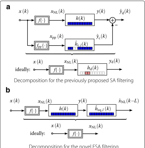
Differences Despite their similarities, the previously proposed SA filtering and the novel ESA filtering employ a fundamentally different mechanism for the estimation of the nonlinearity by an HGM with small temporal sup-port. As depicted in Fig. 7a, classical SA filtering employs a parallel decomposition of the echo path into a direct-path component and a complementary-path component. Can-celing the complementary-part component of the echo signal yields the direct-path component of the echo path,
Fig. 7Decomposition of the echo path into subsystems from which the nonlinearity is estimated:aparallel decomposition for previously proposed SA filtering andbserial decomposition (cascade) for the novel ESA filtering
which is identified efficiently by an HGM for the SA-HGM (recall Section 4.1). As opposed to this, ESA filtering does not rely on any temporal decomposition of the echo path, such that it may be advantageous for non-acoustic system identification, where a dominant direct-path peak does not exist. Instead, the cascade of the Hammerstein sys-tem (a serial decomposition) is employed by augmenting the LEMS with an equalizer (recall blockγ in Fig. 6), as depicted in Fig. 7b. The resulting overall system ideally consists of the first component of the Hammerstein echo path, namely the nonlinearity. This nonlinearity can be identified by an even shorter HGM than for the originally proposed SA filtering and does not require knowledge about any temporal structure of the Hammerstein-shaped echo path’s linear subsystem. Another difference between the proposed SA and ESA filters is that the ESA-HM pro-vides an echo path model with Hammerstein structure (outputeESA(k) in Fig. 6), while the SA-HGM allows to replace the direct-path region of an echo path model with Hammerstein structure by an HGM. This corresponds to the two SA-HGM outputs eHM(k) andeSA(k) in Fig. 5, respectively.
5 Evaluation
In this section, the novel and the previously proposed SA filtering concepts will be compared to each other and to classical adaptive filters in terms of computational com-plexity (Section 5.1) and echo cancellation performance (Section 5.2).
5.1 Computational complexity
This section contains an in-depth analysis of the computa-tional complexity of the previously discussed adaptive fil-ters. In practice, the actual computational load of an algo-rithm is determined by many platform-specific factors, such as the instruction set, the number of clock cycles for a particular arithmetic operation, pipelining, and caching abilities of the processor. Furthermore, especially with growing amount of data to be processed, the memory access pattern may significantly impact how well the pro-cessor exploits its capabilities or waits for new data from external memory. Nevertheless, the number of FLoating Point Operations (FLOPs) is still a commonly accepted indicator for the computational complexity of an algo-rithm on modern platforms, where the different arith-metic operations require similar execution time in prin-ciple. Operations counted as FLOPs will be real-valued multiplications (RMULs), additions (RADDs), and divi-sions (RDIVs).
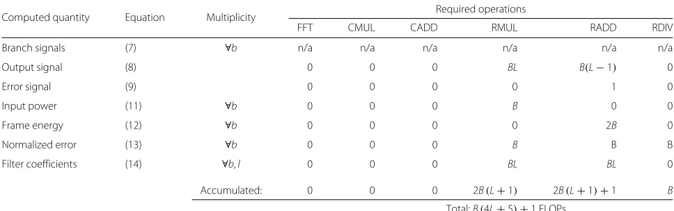
Table 1Computational effort for the identification of an HGM by a time-domain NLMS algorithm
Computed quantity Equation Multiplicity Required operations
FFT CMUL CADD RMUL RADD RDIV
Branch signals (7) ∀b n/a n/a n/a n/a n/a n/a
Output signal (8) 0 0 0 BL B(L−1) 0
Error signal (9) 0 0 0 0 1 0
Input power (11) ∀b 0 0 0 B 0 0
Frame energy (12) ∀b 0 0 0 0 2B 0
Normalized error (13) ∀b 0 0 0 B B B
Filter coefficients (14) ∀b,l 0 0 0 BL BL 0
Accumulated: 0 0 0 2B(L+1) 2B(L+1)+1 B
Total:B(4L+5)+1 FLOPs
(CMUL) by four RMULs and two RADDs. Only for FFT algorithms, where operations performed on the twiddle factors can be cached, an alternative implementation with three RMULs and three RADDs will be considered [63]. Thereby, anNth-order DFT for real-valued time-domain signals can be implemented by
RMULFFT(N)= 1
2Nlog2N− 5 4N RMULs and
RADDFFT(N)= 3
2Nlog2N− 1 4N−4 RADDs [64].
Complexity of adaptive HGM Using these conventions, Table 1 lists the computational effort of the individual operations for the adaptation of an HGM in the time-domain (recall Section 3.2.1).
The first column contains the name of the computed quantity, the second column contains the correspond-ing equation number in this article, the third column
indicates how often the equation has to be evaluated, and the subsequent columns list the number of FFTs, complex-valued, and real-valued operations for the partic-ular equation. Below this list, the accumulated number of individual operations and the total number of FLOPs are listed as well. Note that these operation counts are given per output sample for this time-domain algorithm. The frequency-domain algorithms considered in the following will be analyzed on a frame-wise basis.
Complexity of adaptive PB-HGM Analogously to Table 1, the operations for identifying a PB-HGM accord-ing to Section 3.2.2 in the frequency domain are listed in Table 2. Therein,NN=
N−1 2
+1 denotes the number of non-redundant frequency bins (DC bin to Nyquist bin), for which signal processing is done—the remaining bins can be reconstructed due to the conjugate symmetry. Recall that the operations for a linear model are included in this analysis for the special case ofB=1. Furthermore, the case of a single-partition HGM results forP=1.
Table 2Computational effort for the identification of an HGM by a PB-FNLMS algorithm
Computed quantity Equation Multiplicity Required operations
FFT CMUL CADD RMUL RADD RDIV
Branch signals (21) ∀b n/a n/a n/a n/a n/a n/a
(22) ∀b B 0 0 0 0 0
Output signal (24) 0 BPNN (BP−1)NN 0 0 0
Error signal (23) 2 0 0 0 N2 0
Branch PSDs (25) ∀b 0 0 0 4BNN 2BNN 0
Normalized branch signals (26) ∀b 0 0 0 2BNN BNN BNN
Filter coefficients (27) ∀b,p 0 BPNN BPNN 0 0 0
Filter constraint (28) ∀b,p 2BP 0 0 0 0 0
Accumulated: B+2BP+2 2BPNN NN(2BP−1) 6BNN N2+3BNN BNN
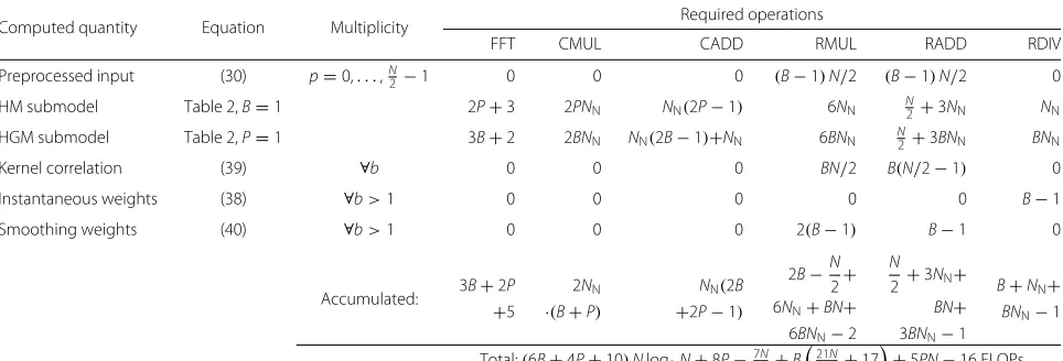
Table 3Computational effort for the identification of a PBSA-HGM with a PB-FNLMS algorithm
Computed quantity Equation Multiplicity Required operations
FFT CMUL CADD RMUL RADD RDIV
Preprocessed input (30) p=0,. . .,N
2 −1 0 0 0 (B−1)N/2 (B−1)N/2 0
HM submodel Table 2,B=1 2P+3 2PNN NN(2P−1) 6NN N2+3NN NN
HGM submodel Table 2,P=1 3B+2 2BNN NN(2B−1)+NN 6BNN N2 +3BNN BNN
Kernel correlation (39) ∀b 0 0 0 BN/2 B(N/2−1) 0
Instantaneous weights (38) ∀b>1 0 0 0 0 0 B−1
Smoothing weights (40) ∀b>1 0 0 0 2(B−1) B−1 0
Accumulated: 3B+2P
+5
2NN
·(B+P)
NN(2B
+2P−1)
2B−N
2+ 6NN+BN+
6BNN−2
N
2+3NN+
BN+
3BNN−1
B+NN+
BNN−1
Total:(6B+4P+10)Nlog2N+8P−72N+B212N+17+5PN−16 FLOPs
Complexity of adaptive SA-HGM The two aforemen-tioned PB-HGM special cases are building blocks for the complexity analysis of the PBSA-HGM (recall Section 4.1), which is listed in Table 3. The additionalNNadditions for the HGM submodel stem from the fact that the HGM submodel’s output has to be added to the complementary-part echo estimate obtained with the HM (recall (35)).
Complexity of adaptive ESA-HM In the same way, the operations for the novel ESA-HM are listed in Table 4. These operations consist of one linear frequency-domain adaptive filter for the HM and one for the echo path inversion, a very short time-domain HGM for assessing loudspeaker nonlinearities, determining the preprocessor weights from the HGM, and evaluating the preprocessor of the HM.
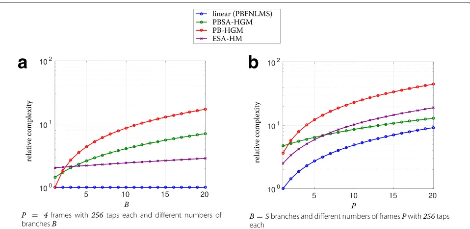
Comparison For consistency with the echo reduction performance evaluation later on, a frame shift ofM=256 taps,B=5 branches,P=4 frames, and onlyLSA=3 taps for the ESA-HM’s HGM submodel are assumed as default. Varying the number of branchesBof the nonlinear mod-els and normalizing the resulting FLOPs to the FLOPs of a linear PB-FNLMS yields the relative FLOPs depicted in Fig. 8a.
Obviously, the ESA-HM has the constant offset of another linear filter for system inversion, which makes it unattractive in comparison to the previously proposed PBSA-HGM for only two or three branches. For two branches, even a full PB-HGM is marginally more effi-cient than an ESA-HM and only slightly more complex than a PBSA-HGM. However, with increasing number of branches, the benefit of an ESA-HM in comparison
Table 4Computational effort for the identification of a ESA-HM with a PB-FNLMS algorithm
Computed quantity Equation Multiplicity Required operations
FFT CMUL CADD RMUL RADD RDIV
Preprocessed input (30) p=0,. . .,N
2 −1 0 0 0 (B−1)N/2 (B−1)N/2 0
HM submodel (forward) Table 2,
B=1 2P+3 2PNN NN(2P−1) 6NN
N
2 +3NN NN
Inversion submodel Table 2,
B=1 2P+3 2PNN NN(2P−1) 6NN
N
2 +3NN NN
Time-domain HGM Table 1,
L=LSA
N
2 0 0 0 2B(LSA+1)N2 2B(LSA+1)N2+N2 BN2
submodel
Kernel correlation (46) ∀b 0 0 0 BLSA B(LSA−1) 0
Instantaneous weights (45) ∀b>1 0 0 0 0 0 B−1
Smoothing weights (47) ∀b>1 0 0 0 2(B−1) B−1 0
Accumulated: 4P+6 4PNN NN(4P−1)
2B+12NN+
N(B−1) 2 +BLSA+
BN(LSA+1)−2
N+6NN+
BLSA+
3BN
2 +
BLSAN−1
B+
2NN+
BN
2 −1 Total:(8P+12)Nlog2N+16P+2N+2LSA+72N+2LSAN+3
Fig. 8Relative number of FLOPs for system identification with different models, revealing a significant complexity reduction by ESA filtering for a low number of frames (even without block partitioning) and for a high number of branches. The relative FLOPs result from normalization to the FLOPs of a linear model withP=4 partitions in (a) andP=1 partition in (b)
to a PB-HGM or even to the less complex PBSA-HGM becomes evident: an ESA-HM’s complexity is mainly dominated by the two linear adaptive filters—even for
B=20 branches.
Varying the number of frames P and leaving B = 5
constant results in the relative FLOPs depicted in Fig. 8b, where relative FLOPs result from normalization to the FLOPs of an adaptive linear model with a single parti-tion. As can be seen, the ESA-HM leads to a significantly reduced computational complexity for a low number of framesP. Thus, the ESA-HM always leads to a
complex-ity reduction compared to the PB-HGM, even forP = 1,
which corresponds to conventional frequency-domain adaptive filtering without block partitioning.
5.2 Echo reduction performance
In this section, the echo reduction performance of the novel ESA and the previously proposed SA filtering con-cept will be compared to classical adaptive filters based on linear models and HGMs.
5.2.1 Experimental setup
The following evaluation is based on double-talk free recordings of male and female speech, played-back and recorded with a smartphone in hands-free mode at very high volume. In total, five different physical setups, referred to as setups A to E, will be considered. The acous-tically relevant characteristics of these setups are listed in Table 5.
Setups A and B correspond to recordings with a dura-tion of about 130 s in a living room-like environment. Setups A and B differ in the placement of the smartphone within the same environment. Setup C corresponds to a recording in an anechoic environment and has a duration of about 80 s. The data for setups D and E are synthesized by convolving the anechoic nonlinear recordings obtained from setup C with measured RIRs. The employed RIRs are from a lab environment with variable acoustics, once with curtains at the walls (setup D) and once with open curtains (setup E). For all setups, a partitioned-block lin-ear model (PB-HGM with a single linlin-ear branch), a full PB-HGM (full temporal support), a PBSA-HGM, and an ESA-HM will be compared.
In the following experiments, processing is done at a sampling rate offS=16 kHz. The acoustic echo paths are estimated with FIR filters of lengthL=1024 taps and the input signals and impulse responses are partitioned into P = 4 blocks with a relative frame shift ofM=256 taps
Table 5Properties of setups A to E for the AEC experiments
Room type T60 Room dimensions
Setup A Living room 900 ms 4×5×2.5 m
Setup B Living room 900 ms 4×5×2.5 m
Setup C Anechoic chamber n/a 2×2×2 m
Setup D Lab environment with curtains on walls
250 ms 5.5×5.7×3.1 m
(implyingN = 512). Note that, despite large values of T60 for some setups, the echo reduction performance in the experiments is not limited by the filter length but by the nonlinearity of the echo path (see Section 5.2.2 for a quantitative analysis of the amount of nonlinearity in the recordings).
As in [20], the HGMs consist of B = 5 branches,
with odd-order Legendre polynomials up to order 9 as nonlinearity basis functions fb{·} in (5). The algorithm parameters used in the experiments have been selected based on the recordings of setup C. In particular, a step-size ofμb = 0.1 (see (26)) is used for the kernels of the
PB-HGMs and a stepsize of μb = 0.2 is used for the
PBSA-HGMs and ESA-HMs. For the reference algorithm, consisting of the linear filter, a stepsize of μ1 = 0.5 is employed to account for the lack of multiple adaptation branches. Furthermore, the adaptation process is refined using the robust statistics described in [34, 59], which hardly affects the computational complexity but robusti-fies the system identification against outliers in the error signal. For the same purpose, the dynamics of the adaptive preprocessor weights is limited to a maximum stepsize of
±0.001 per frame.
The AEC performance is quantified by computing the Echo-Return Loss Enhancement (ERLE) measure [62]
ERLE=10 log10
whereyecho(k)is the echo signal component of the micro-phone signaly(k)andyˆ(k)is the echo estimate obtained using the model to be evaluated (linear model, PB-HGM, PBSA-HGM, ESA-HM). For single talk, (50) becomes
ERLE=10 log10
where the numerator is the power of the microphone signal y(k) and the denominator is the power of the error signal e(k) produced by the model to be evalu-ated. For a practical evaluation, the mathematical expec-tation (ensemble average) in (51) will be replaced by a time-averaging over the entire sequences. Note that the ERLE measure in its general definition of (50) does not depend on the near-end signal components (including the number and positions of the near-end sources) but requires knowledge of the actual far-end signal compo-nent during double-talk periods. This knowledge is not available in practice. Nonetheless, the ERLE performance during double-talk periods can be simulated by perform-ing AEC on sperform-ingle-talk recordperform-ings with previously deter-mined fixed filters (as will be done in Section 5.2.3 in experiment 2).
5.2.2 Quantification of nonlinearity
For monofrequent excitation signals, the nonlinearity of a system can easily be assessed by means of the Total Harmonic Distortion (THD), which measures the ratio of the energy of the excitation frequency to the energy of its harmonics. However, for nonstationary broadband exci-tation signals like speech, this measure is not meaningful anymore. In order to characterize the nonlinearity nev-ertheless, one can pursue noise-loading methods [65] or, as done in the following, methods based on the actual AEC excitation signal itself. To this end, consider the energyEinwhich is recorded in the bandwidth excited by the digital loudspeaker signal (0−8 kHz) and the energy Eout which is recorded above for frequencies exceeding the highest frequency contained in the excitation signal (8−16 kHz). For a linear system, the out-of-band energy is only caused by noise. For a nonlinear system,Eoutis sig-nificantly increased due to the harmonic distortion. The In-band/Out-of-band Ratio (IOR)
may therefore serve as a measure of the intensity of the nonlinearity in the echo signal.
Furthermore, the so-called Linear-to-Non-Linear Ratio (LNLR) is defined as the ratio between the power of the linear echo signal component and the power of the nonlinear echo signal component. Thus, a lower LNLR corresponds to stronger nonlinearities. While the THD is a description of how much nonlinearity a particular frequency causes at its harmonics, a frequency-selective LNLR quantifies the distortion present at a particular fre-quency4. Although an exact LNLR computation required exact knowledge of the linear and nonlinear system com-ponents to compute the respective signal comcom-ponents, the LNLR can be estimated using the echo estimateyˆ(k) obtained by a converged long adaptive linear filter and the resulting error signale(k) = y(k)− ˆy(k). Employing the respective signal spectra estimates Syˆyˆ(f)andSee(f), the LNLR at a frequencyf can be estimated as
LNLR(f)=10 log10
The particular smartphone employed for the AEC experiments leads to an IOR of 27 dB for the AEC speech signal in an anechoic environment5. The LNLR estimated from the same measurement is depicted in Fig. 9 up to 8 kHz—for higher frequencies, the numerator of (52) is determined by noise only and, therefore, (52) cannot be employed to estimate the LNLR anymore.
Fig. 9Estimated frequency-selective linear-to-nonlinear ratio according to (52) for the particular smartphone and excitation signal (speech) used during the AEC experiments
a local minimum and the maximum of the far-end signal spectrum, respectively.
5.2.3 Experimental results
In the following, two experiments will be discussed. Experiment 1 considers an adaptive identification of the nonlinear systems according to Section 5.2.1, and exper-iment 2 considers an offline filtering without further adaptation with previously adapted models from the end of experiment 1. While experiment 1 is affected by the initial convergence phase, experiment 2 evaluates the per-formance achievable in double-talk situations after con-vergence of the filters, which is of vital importance for a full-duplex voice communication system as well.
Experiment 1 - continuously adapted filters Figure 10a shows the ERLE measure for different setups and models
for experiment 1. Note that the PBSA-HGM is listed twice: once with the previously considered output signaleSA(k) and once with the HM submodel’s outputeHM(k). Obvi-ously, the linear filter performs worst for all setups. The other end of the scale is represented by the PB-HGM, which leads to an almost twice as high average ERLE value for setup C. The PBSA-HGM leads to a good approxima-tion of the PB-HGM. In setups A and B, the PB-HGM with full temporal support is even marginally outper-formed by the PBSA-HGM’s HM and HGM outputs, respectively. On the other hand, when considering the HM submodel of the PBSA-HGM only, the average gap to the PB-HGM performance is larger. This is not surprising, as the classical PBSA-HGM with a peak-modeling HGM has more degrees of freedom and tracks the nonlinear-ities before providing a smoothed nonlinearity estimate to the HM submodel. The ESA-HM can also approxi-mate the PB-HGM but leads to slightly less ERLE than the PBSA-HGM’s HM output in experiment 1. Yet, the ESA-HM consistently outperforms the partitioned block linear filter. This clearly verifies the applicability of SA fil-tering in general and of the proposed novel ESA filfil-tering concept for practically relevant scenarios with real-world smartphone recordings.
Experiment 2 - echo reduction during double talk In experiment 2 (depicted in Fig. 10b), when processing the entire sequence offline with the converged filters from the previous experiment, the ESA-HM performs as good as the full PB-HGM in setups C and D. Only in setups A and E, the PBSA-HGM can marginally outperform the
ESA-HM in experiment 2. Overall, the ESA-HM gener-alizes slightly better for double-talk situations than the HGM. Interestingly, the typically considered PBSA-HGM’s HGM output and the PBSA-PBSA-HGM’s HM output do not differ significantly in experiment 2, which supports the initial assumption that an HM is a suitable efficient approximation of the echo path. The increased perfor-mance due to the PBSA-HGM’s HGM submodel seems to originate from a quicker reaction to the instantaneous signal characteristics.
Clearly, the novel ESA-HM is a very well performing alternative to the PBSA-HGM, which leads to comparable or even better echo reduction in double-talk situations.
6 Conclusions
The adaptation of nonlinear echo paths for small portable devices requires efficient adaptive nonlinear echo path models. To this end, a novel variant of SA filtering has been introduced and compared to known concepts in this article. This novel ESA filtering method, leading to an adaptive ESA-HM, exploits the inability of IRs to model nonlinearities to obtain an estimate of the unobservable nonlinearly distorted loudspeaker signal by inverse fil-tering. While the previously proposed PBSA-HGM has been an efficient alternative to HGMs only for a block-partitioning of the filter, the novel ESA filtering concept is advantageous without block partitioning at all and for a very high number of branches (see complexity analy-ses in Section 5.1). For applications where very long RIRs need to be modeled and where a low input-output delay is required, a block partitioning and therefore the PBSA-HGM may computationally be more efficient than the ESA-HM. Both methods thereby complement each other very well in terms of computational efficiency for dif-ferent application scenarios. A comparison of the echo reduction performance of the ESA-HM, the PBSA-HGM, a linear model, and a PB-HGM in Section 5.2 has empha-sized the efficacy of the proposed ESA-HM, especially for double-talk situations, in which AEC is actually most important.
Endnotes
1Note that this representation of a Volterra filter is also
referred to as diagonal coordinate representation [66].
2This update rule is also referred to as NLMS with
kernel-specific normalization in [66].
3As opposed to time-domain adaptive filters, the
com-plexity for filter adaptation in the frequency domain is not determined by the length of the time-domain support of the filter, but by the DFT sizeNand the number of parti-tionsP. This disqualifies unpartitioned frequency-domain adaptive filters, as the HGM submodel in Fig. 5 would
have the same complexity as the HGM with full temporal support in Fig. 2d.
4Determining such a measure is also referred to as
Schüßler’s model in [67], as it goes back to [68, 69]. 5Note that this number is caused by nonlinearity and
not by background noise, as the SNR of the recorded sig-nal is more than 24 dB in the 8−16 kHz range, whereEout is computed.
Acknowledgements
The authors would like to thank the Deutsche Forschungsgemeinschaft (DFG) for supporting this work (contract number KE 890/9-1).
Competing interests
The authors declare that they have no competing interests.
Received: 26 June 2016 Accepted: 6 October 2016
References
1. MM Sondhi, An adaptive echo canceller. Bell Syst. Tech. J.46(3), 497–511 (1967)
2. P Dreiseitel, E Hänsler, H Puder, inProc. European Signal Process. Conf. (EUSIPCO). Acoustic echo and noise control—a long lasting challenge (EURASIP, Rhodes, 1998), pp. 945–952
3. EJ Thomas, Some considerations on the application of the Volterra representation of nonlinear networks to adaptive echo cancellers. Bell Syst. Tech. J.50(8), 2797–2805 (1971)
4. A Stenger, L Trautmann, R Rabenstein, inProc. IEEE Intl. Conf. Acoustics, Speech, Signal Process. (ICASSP). Nonlinear acoustic echo cancellation with 2nd order adaptive Volterra filters, vol. 2 (IEEE, Phoenix, 1999), pp. 877–880 5. M Zeller, LA Azpicueta–Ruiz, J Arenas-Garcia, W Kellermann, Adaptive
Volterra filters with evolutionary quadratic kernels using a combination scheme for memory control. IEEE Trans. Signal Process.59(4), 1449–1464 (2011)
6. AN Birkett, RA Goubran, inProc. IEEE Workshop Neural Networks Signal Process. (NNSP). Nonlinear echo cancellation using a partial adaptive time delay neural network (IEEE, Cambridge, 1995), pp. 449–458
7. LSH Ngja, J Sjobert, inProc. IEEE Intl. Conf. Acoustics, Speech, Signal Process. (ICASSP). Nonlinear acoustic echo cancellation using a Hammerstein model (IEEE, Seattle, 1998), pp. 1229–1232
8. D Comminiello, M Scarpiniti, R Parisi, A Uncini, inProc. Int. Workshop Acoustic Echo, Noise Control (IWAENC). A functional link based nonlinear echo canceller exploiting sparsity (IWAENC, Tel Aviv, 2010)
9. D Comminiello, M Scarpiniti, LA Azpicueta-Ruiz, J Arenas-Garcia, A Uncini, Functional link adaptive filters for nonlinear acoustic echo cancellation. IEEE Trans. Audio Speech Lang. Process.21(7), 1502–1512 (2013) 10. G Li, C Wen, WX Zheng, Y Chen, Identification of a class of nonlinear
autoregressive models with exogenous inputs based on kernel machines. IEEE Trans. Signal Process.59(5), 2146–2159 (2011)
11. J Kivinen, AJ Smola, RC Williamson, Online learning with kernels. IEEE Trans. Signal Process.52(8), 165–176 (2004)
12. AN Birkett, RA Goubran, inProc. IEEE Workshop Applications Signal Process. Audio Acoustics (WASPAA). Limitations of handsfree acoustic echo cancellers due to nonlinear loudspeaker distortion and enclosure vibration effects (IEEE, New Paltz, 1995), pp. 103–106
13. A Stenger, R Rabenstein, inProc. European Signal Process. Conf. (EUSIPCO). An acoustic echo canceller with compensation of nonlinearities, vol. 98 (EURASIP, Island of Rhodes, 1998), pp. 969–972
14. A Stenger, W Kellermann, Adaptation of a memoryless preprocessor for nonlinear acoustic echo cancelling. Signal Process.80(9), 1747–1760 (2000)
15. S Malik, G Enzner, State-space frequency-domain adaptive filtering for nonlinear acoustic echo cancellation. IEEE Trans. Audio Speech Lang. Process.20(7), 2065–2079 (2012)