Takuya Hayashi1, Takeshi Shimoyama2,
Naoyuki Shinohara3, and Tsuyoshi Takagi1
1
Kyushu University, 744, Motooka, Nishi-ku, Fukuoka 819-0395, Japan.
2
FUJITSU LABORATORIES Ltd., 4-1-1, Kamikodanaka, Nakahara-ku, Kawasaki, 211-8588, Japan.
3
National Institute of Information and Communications Technology, 4-2-1, Nukui-kitamachi, Koganei, Tokyo, 184-8795, Japan.
Abstract. There are many useful cryptographic schemes, such as ID-based encryption, short signature, keyword searchable encryption, attribute-based encryption, functional encryption, that use a bilinear pair-ing. It is important to estimate the security of such pairing-based cryptosystems in cryptography. The most essential number-theoretic problem in pairing-based cryptosystems is the discrete logarithm problem (DLP) because pairing-based cryptosystems are no longer secure once the underlining DLP is broken. One efficient bilinear pairing is the ηT pairing defined over a supersingular elliptic curveE on the finite field
GF(3n) for a positive integern. The embedding degree of theη
T pairing is 6; thus, we can reduce the DLP overE onGF(3n) to that over the finite fieldGF(36n). In this paper, for breaking theηT pairing overGF(3n), we discuss solving the DLP overGF(36n) by using the function field sieve (FFS), which is the asymptotically fastest algorithm for solving a DLP over finite fields of small characteristics. We chose the extension degree n = 97 because it has been intensively used in benchmarking tests for the imple-mentation of theηT pairing, and the order (923-bit) ofGF(36·97) is substantially larger than the previous world record (676-bit) of solving the DLP by using the FFS. We implemented the FFS for the medium prime case (JL06-FFS), and propose several improvements of the FFS, for example, the lattice sieve for JL06-FFS and the filtering adjusted to the Galois action. Finally, we succeeded in solving the DLP over
GF(36·97). The entire computational time of our improved FFS requires about 148.2 days using 252 CPU
cores. Our computational results contribute to the secure use of pairing-based cryptosystems with theηT pairing.
Keywords: pairing-based cryptosystems,ηT pairing, discrete logarithm problems, function filed sieve
1
Introduction
After the advent of the tripartite Diffie-Hellman (DH) key exchange scheme [20] and ID-based encryption using pairing [11], plenty of attractive pairing-based cryptosystems have been proposed, for example, short signature [13], keyword searchable encryption [10], efficient broadcast encryption [12], attribute-based encryp-tion [29], and funcencryp-tional encrypencryp-tion [27]. Pairing-based cryptosystems have become a major research topic in cryptography.
Pairing-based cryptosystems are constructed on the groupsG1,G′1andG2of the same order with a bilinear
pairingG1×G′1→G2. The security of pairing-based cryptosystems is based on the difficulty in solving several
number-theoretic problems such as the computational/decisional bilinear DH problem (CBDH/DBDH), strong DH problem (SDH), decisional linear problem (DLIN), and symmetric external DH problem (SXDH). However, the most important number-theoretic problem in pairing-based cryptosystems is the discrete logarithm problem (DLP) onG1,G′1, andG2. All the other number-theoretic problems above are no longer intractable once the
DLP onG1,G′1, or G2is broken. Therefore, it is important to investigate the difficulty in solving the DLP.
One of the most efficient algorithms for implementing the pairing is theηT pairing [5] defined over a super-singular elliptic curve E on the finite field GF(3n), wherenis a positive integer. Since the embedding degree of E is 6, the ηT pairing can reduce a DLP over E on GF(3n), which is called an ECDLP, to a DLP over
GF(36n). Joux proposed the (probably) first cryptographic scheme [20] that uses the pairing overE. Boneh et al.then applied the pairing overE to the short signature scheme [13], where a point (x, y) onE for extension degreen= 97 can be represented as a signature value, e.g.,x=KrpIcV0O9CJ8iyBS8MyVkNrMyE. At CRYPTO 2002, Barreto et al. presented algorithms for efficiently computing Tate pairing overE [6]. Many high-speed implementations of pairing overE have subsequently been proposed [3, 7–9, 17, 18, 24]. For many of these im-plementations, benchmark tests using the extension degreen= 97 have been conducted. Therefore, we focus on the DLP over finite fieldGF(36·97) in this paper. The cardinality of the subgroup of the supersingular elliptic
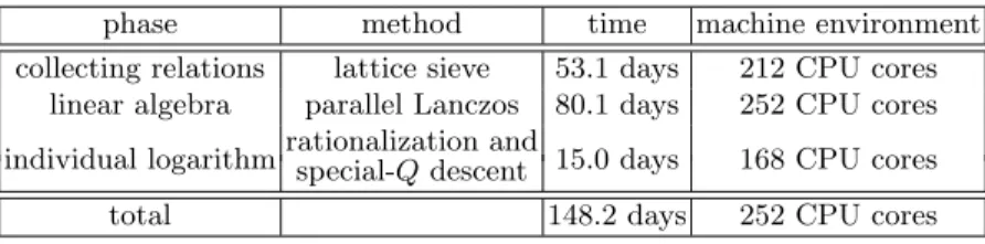
Table 1.Summary of time data for solving DLP overGF(36·97)
phase method time machine environment collecting relations lattice sieve 53.1 days 212 CPU cores
linear algebra parallel Lanczos 80.1 days 252 CPU cores
individual logarithmrationalization andspecial-Qdescent 15.0 days 168 CPU cores
total 148.2 days 252 CPU cores
previous world record of solving the DLP overGF(36·71), whose cardinality is 676 bits [19]. The current world
record for solving an ECDLP is the 112-bit ECDLP [14]. Pollard’s ρ method is used for solving the 112-bit ECDLP, and has not reached the ability for solving the 151-bit ECDLP over the subgroup ofE.
In this paper, we analyze the difficulty in solving the DLP overGF(36·97) by using the function field sieve
(FFS), which is known as the asymptotically fastest algorithm [1, 2]. Since the FFS proposed by Joux and Lercier (JL06-FFS) [23] is suitable for solving the DLP over a finite field whose characteristic is small, we use the JL06-FFS and propose several efficient techniques for increasing its speed. Note that the FFS generally consists of four phases: polynomial selection, collecting relations, linear algebra, and individual logarithm, and the time-consuming phases are collecting relations and linear algebra. For the collecting relations phase, we applied several techniques; lattice sieve for the JL06-FFS, lattice sieve with single instruction multiple data (SIMD), and optimization for our parameters. These techniques enable the sieving program to run about 6 times faster. In the linear algebra phase, we applied careful treatments of singleton-clique and merging [15] to the Galois action originating from extension degree 6 ofGF(36·97), with which the size of the matrix used for the Lanczos method is reduced to approximately 30%. By implementing the JL06-FFS with our improvements, we succeeded in solving the DLP overGF(36·97) by using 252 CPU cores (Core2 quad, Xeon, etc) for the target
problem discussed in Section 3.1. As shown in Table 1, the computations required 53.1 days for the collecting relations phase, 80.1 days for the linear algebra phase, and 15.0 days for the individual logarithm phase. Thus, a total of 148.2 days were required to solve the DLP overGF(36·97) by using 252 CPU cores. Our computational
results contribute to the secure use of pairing-based cryptosystems with theηT pairing.
This paper is organized as follows: In Section 2, we describe the paring-based cryptosystems, the DLP, and an overview of the FFS. In Section 3, we present our target problem of the DLP overGF(36·97) and the parameter
settings used for our implementation of the FFS. In Section 4, we propose our efficient implementation techniques for the lattice sieve and the parallel Lanczos method. In Section 5, we report the computational results of our implementation of solving the target problem overGF(36·97). Finally we give concluding remarks and a rough
estimation for larger key sizes.
2
Pairing-based cryptosystems and discrete logarithm problem (DLP)
In this section, we briefly explain the security of pairing-based cryptosystems and give a general overview of the function field sieve (FFS). We also mention its parameters such as the smoothness boundB.
Before beginning the discussion, we define the discrete logarithm problem (DLP) over a finite field. Let gF be a generator of a large multiplicative subgroupGF of a finite field. For a givenTF ∈GF, a DLP over GF is the problem of computing an integerX such thatTF =gFX. Generally,X is described as loggF TF.
The ECDLP is also defined in the same manner using the additive group operation. LetGE be a generator of a subgroup GE of an elliptic curve E on a finite field and assume that TE ∈ GE is given. An ECDLP is defined as the problem of computing an integer Y satisfyingTE = [Y]GE. In this case, we also describe Y as logG
ETE.
2.1 Pairing-based cryptosystems and DLP
In particular, theηT pairing is a bilinear map such thatηT :G1×G1→G2, whereG1is an additive subgroup
of a supersingular elliptic curve overGF(3n),G
2is a cyclic subgroup ofGF(36n)∗, and the cardinalities ofG1, G2 are the same prime number P. The security of pairing-based cryptosystems with theηT pairing depends on the difficulty of not only an ECDLP over G1 but also a DLP over G2 by MOV reduction. To explain
this fact, we take based encryption constructed on pairing-based cryptosystems as an example. The ID-based encryption has a master key skey ∈ ZP. Each user ID is deterministically transformed into a point
QID ∈ G1, and the secret key SID is defined by [skey]QID. Therefore, solving the ECDLP over G1, namely SID= [skey]QID, we obtain the master keyskey = logQIDSID. Additionally, for an arbitrary point R ∈G1, we
computeηT(SID,R), ηT(QID,R)∈G2, and then haveηT(SID,R) =ηT([skey]QID,R) =ηT(QID,R)skey ∈G2.
This implies thatskey = logηT(QID,R)ηT(SID,R) is also available by solving the DLP over G2. In this paper,
we discuss the DLP over a subgroup ofGF(36n)∗.
2.2 General overview of FFS
The FFS is the asymptotically fastest algorithm for solving a DLP over finite fields of small characteristics. Adleman proposed the first FFS in 1994 [1]. After that, several variants of the FFS have been proposed; Adleman and Huang improved the FFS [2], and Joux and Lercier proposed two more practical FFS’s, JL02-FFS [22] and JL06-FFS [23]. The details of JL06-FFS are explained in Sections 3.2.
In this section, we give a general overview of an FFS that consists of four phases: polynomial selection, collecting relations, linear algebra, and individual logarithm. In the overview, we aim at computing loggT whereT ∈ ⟨g⟩ ⊂GF(36n)∗.
Polynomial selection phase: We select κ from κ = 1,2,3,6 for the coefficient field of GF(3κ)[x], and a bivariate polynomialH(x, y)∈GF(3κ)[x, y] such thatH satisfies the eight conditions proposed by Adleman [1] and degyH =dH for a given parameter valuedH. We compute a random polynomial m∈GF(3κ)[x] of degree
dmand a monic irreducible polynomialf ∈GF(3κ)[x] such that
H(x, m)≡0 (mod f), degf = 6n/κ. (1)
We then haveGF(36n)∼=GF(3κ)[x]/(f). Moreover, there is a surjective homomorphism
ξ:
{
GF(3κ)[x, y]/(H) → GF(36n)∼=GF(3κ)[x]/(f)
y 7→ m.
We select a positive integerBas a smoothness bound, and define a rational factor baseFR(B) and an algebraic factor baseFA(B) as follows.
FR(B) ={p∈GF(3κ)[x]| deg(p)≤B,pis monic irreducible}, (2)
FA(B) ={⟨p, y−t⟩ ∈Div(GF(3κ)[x, y]/(H))|p∈FR(B), H(x, t)≡0 (modp)}, (3)
where Div(GF(3κ)[x, y]/(H)) is the divisor group ofGF(3κ)[x, y]/(H) and⟨p, y−t⟩is a divisor generated by
pand y−t. Note thatFR(0) =FA(0) ={∅}. We simply call the setFR(B)∪FA(B) a factor base and the set
FR(k)\FR(k−1)∪FA(k)\FA(k−1) a factor base of degree kfork= 1,2, . . . , B.
Collecting relations phase: We select positive integersR, S and collect a sufficient amount of pairs (r, s)∈ (GF(3κ)[x])2 such that
degr≤R,degs≤S,gcd(r, s) = 1, (4)
rm+s= ∏ pi∈FR(B)
pai
i , (5)
⟨ry+s⟩= ∑
⟨pj,y−tj⟩∈FA(B)
bj⟨pj, y−tj⟩, (6)
for some non-negative integersai, bj by using a sieving algorithm such as the lattice sieve discussed in Section 4.1. To efficiently computebj in (6), we use the following equivalent property instead of (6):
(−r)dHH(x,−s/r) = ∏
⟨pj,y−tj⟩∈FA(B)
pbj
The (r, s) satisfying (4), (5), and (7) is called aB-smooth pair. Lethbe the class number of the quotient field ofGF(3κ)(x)[y]/(H) and assume thathis coprime to (36n−1)/(3κ−1). Then the following congruent holds:
∑
pi∈FR(B)
ailoggpi≡
∑
⟨pj,y−tj⟩∈FA(B)
bjloggsj (mod (36n−1)/(3κ−1)), (8)
where sj = ξ(tj)1/h, ⟨tj⟩= h⟨pj, y−tj⟩. We call the congruent (8) “relation” in this paper. Moreover, free relation [19] provides additional relations without computation with a sieving algorithm.
Linear algebra phase: We generate a system of linear equations described as a large matrix from those collected relations and reduce the rank of the matrix by filtering [15]. The reduced system of linear equations is solved using the parallel Lanczos method [4, 19] or other methods, and the discrete logarithms of elements in the factor base are obtained:
loggp1, ...,loggp#FR(B),loggs1, ...,loggs#FA(B).
Individual logarithm phase: Note that our goal is to compute loggT. Therefore, we find integersai, bj such that
loggT ≡ ∑
pi∈FR(B)
ailoggpi+
∑
⟨pj,y−tj⟩∈FA(B)
bjloggsj (mod (36n−1)/(3κ−1)), (9)
using the special-Q descent [23]. The computational time for the individual logarithm phase is smaller than those for the collecting relations and linear algebra phases.
3
Target problem for
n
= 97 and setting of parameters for FFS
We discuss solving the DLP over a subgroup ofGF(36·97)∗, where the cardinality of the subgroup is 151 bits.
To estimate the time complexity of solving such a DLP, we unintentionally set a target problem determined from the circular constant π and natural logarithm e. The details are explained in Section 3.1. To solve the target problem effectively, we select the parameter values of the FFS and estimate important numbers, e.g., the number of elements in the factor base, for it. The details are given in Section 3.2.
3.1 Target problem
For pairing-based cryptosystems, many high-speed implementations of theηT pairing over supersingular elliptic curves onGF(3n) have been reported [3, 6–9, 17, 18, 24], and many benchmark tests using theη
T pairing have been conducted forGF(397). In this paper, we deal with a supersingular elliptic curve defined by
E:={(x, y)∈GF(397)2 : y2=x3−x+ 1} ∪ {O},
where O is the point at infinity. The order of the E is 397+ 349+ 1 = 7P
151 where P151 is a 151-bit prime
number as follows:
P151= 2726865189058261010774960798134976187171462721.
Next, letG1be the subgroup ofE of orderP151and letG2 be the subgroup ofGF(36·97)∗ of orderP151. Note
that, since orders ofG1 andG2are prime numbers, every element ofG1\{O}andG2\{1}is a generator ofG1
andG2, respectively. TheηT pairing forn= 97 is a map fromG1×G1 toG2.
Our goal is to solve the ECDLP in G1. To set our target problem unintentionally, we select two elements Qπ,QeinG1, which correspond to the circular constantπand natural logarithme, respectively. We explain how
we selectQπ andQeas follows. First, we describeGF(397) asGF(3)[x]/(x97+x16+ 2), where the irreducible polynomial x97+x16+ 2∈GF(3)[x] is well used for the fast implementation of field operations. An element in GF(397) is represented by∑96
i=0dixi, wheredi∈GF(3) ={0,1,2}. To transform πand eto an element in
GF(397) respectively, we define a bijective mapϕ:∑96
i=0dixi7→
∑96
i=0di3i∈Z. We then transformπandeto the 3-adic integer of 97 digits as follows:
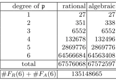
Table 2.Number of elementspinFR(B) andFA(B) ofB= 6
degree ofp rational algebraic
1 27 27
2 351 338
3 6552 6552
4 132678 132496 5 2869776 2869776 6 64566684 64563408 total 67576068 67572597 #FR(6) + #FA(6) 135148665
From these values, we defineQπ = (xπ, yπ) andQe= (xe, ye)∈G1as follows. We first find the non-negative
smallest 3-adic integers cπ andce such thatϕ−1(⌊π·395⌋+cπ) andϕ−1(⌊e·396⌋+ce) become x-coordinates of the elements Qπ and Qe in the subgroup G1 on the E. In fact we can set xπ = ϕ−1(⌊π·395⌋+(11)3)
and xe = ϕ−1(⌊e·396⌋+(120)3). There are two points in G1\{O}of the same x-coordinate. We then set the
correspondingy-coordinate by computingyπ = (x3π−xπ+ 1)(3
97+1)/4
andye= (x3e−xe+ 1)(3
97+1)/4
inGF(397), respectively. These values are checkable by scripts given in Appendix B.
Again, our goal is to solve the ECDLP inG1, i.e., for given Qπ, Qe∈G1we try to find integerssuch that
Qπ= [s]Qe. (10)
On the other hand, theηT pairing enables us to reduce the ECDLP inG1to the DLP overG2by the relationship ηT(Qπ,Qπ) =ηT(Qπ,Qe)s. Therefore, we can findsby computing the discrete logarithm
s= logη
T(Qπ,Qe)ηT(Qπ,Qπ) = loggηT(Qπ,Qπ)/loggηT(Qπ,Qe) modP151, (11)
for a generatorgofG2.
3.2 Parameter settings for FFS
In this section, we explain the parameter setting used for our implementations of the FFS. Hayashiet al.[19] reported that, whenn≤509, the JL06-FFS [23] is more efficient for solving the DLP overGF(36n) than the JL02-FFS [22]. Thus, we use the JL06-FFS for our computation. In the JL06-FFS, the condition that “r is monic” is introduced into the collecting relations phase in order to compute efficiently. For the remainder of this paper, the FFS refers to the JL06-FFS.
To solve our DLP over GF(36·97), we have to select several parameter values of the FFS, such that its
computational time is small enough for a fixed extension degreen. The parameter values forn= 97 are listed in [30, Table 3], and we use those parameter values for our computation.
We can select the parameterκof the FFS to describeGF(36·97) asGF(3κ)[x]/(f), whereκis in{1,2,3,6} andf ∈GF(3κ)[x] is an irreducible polynomial of degree 6·97/κ. The appropriate value ofκis given in [30, Table 3], i.e.,κ= 6. However, we selectκ= 3 for the following reasons. In the linear algebra phase, filtering [15] is performed to reduce the size of the matrix. Then it is required that all elements in the factor base correspond to the memory addresses of the PC for efficient computation. The number of elements in the factor base for
κ= 6 is much larger than that forκ = 3, so κ= 3 is advantageous on this point. Additionally, [30, Table3] shows that the computational cost of the FFS for κ= 3 is only about twice as much as that forκ = 6. We conducted test runs forκ= 3,6 in the collecting relations phase. We then noticed that our implementation for
κ= 3 was much faster than forκ= 6, so we setκ= 3. For the remainder of the paper,κ= 3.
Polynomial selection phase: We select the bivariate polynomial H(x, y) of the form x+ydH for a given
parameterdH of the FFS in the same manner as [19]. Then we search an irreducible polynomialf ∈GF(3κ)[x] of degree 6·97/κby factoringH(x, m) for a random polynomialm∈GF(3κ)[x] whose degree isdm. In fact, we randomly pick upmfromGF(3)[x], so thatf is also in GF(3)[x] for use of the Galois action. From [30, Table 3], we setdH and dm as 6 and 33, respectively. The polynomialsf and m, which we used in our experiments, are provided in Appendix B.
Collecting relations phase: In the collecting relations phase, we use the lattice sieve [28] and the free relation [19] and collect many relations (8); (r, s)∈(GF(3κ)[x])2 satisfying (4), (5), (7), wherer is monic. The search
range for the lattice sieve depends on the maximum degrees R, S of r, s. We set R = S = 6 based on [30, Table 3]. The lattice sieve gives a certain amount of relations for one special-Q, which is defined in Section 4.1. Therefore, we require a sufficient number of special-Q’s so that the number of relations obtained in the collecting relations phase is larger than that of all elements in the factor base. The minimum sufficient number of
special-Q’s is estimated by the following process. We have to select special-Q’s from the subset FR(6)\FR(5), whose cardinality is 64566684 (See Table 2). Letθmin be the minimum sufficient ratio of special-Q’s over all elements in FR(6)\FR(5). Forn= 97 andκ= 3, we can estimateθmin = 0.01292 [30, Table 3]. Therefore, the number of special-Q’s must be larger than⌈0.01292·64566684⌉= 834202. In our computation, we set 2500000 as the number of special-Q’s to obtain more relations than we require since we expect that these excess relations will help us reduce the size of the matrix during filtering, especially in singleton-clique.
4
Implementation
In this section, we propose the following efficient implementation techniques; the lattice sieve for JL06-FFS and optimization for our parameters in the collecting relations phase, the data structure and the parallel Lanczos method for the Galois action in the linear algebra phase, for reducing the computational cost of the FFS for solving the DLP overGF(36·97). Parameters (κ, d
H, dm, B, R, S) are fixed as (3,6,33,6,6,6). The reasoning for this is explained in Section 3.2.
4.1 Collecting relations phase
In the collecting relations phase, we used the lattice sieve [28] in a similar fashion to factoring a large integer [25] and solving discrete logarithm problems [21, 22]. We give an overview of our implementation of the lattice sieve in the following paragraphs, and more details are described in Appendix A.
Lattice sieve for JL06-FFS: Sieving with the lattice sieve is performed for (r, s)∈(GF(33)[x])2 such that
the formula (5) given in Section 2.2 is divisible by an element Q chosen from a subset of the rational factor baseFR(6)\FR(5) (thisQis called a “special-Q”). Recall that degrand degsare not greater thanR= 6 and
S= 6, respectively. Such (r, s) can be represented as (r, s) =c(r1, s1) +d(r2, s2) for given reduced lattice bases
(r1, s1),(r2, s2)∈(GF(33)[x])2 and anyc, d∈GF(33)[x] such that deg(cr1+dr2)≤6,deg(cs1+ds2)≤6, then
sieving is done on the boundedc-dplane. After sieving, we conduct the smoothness test [16] for “candidates” that are evaluated as B-smooth pairs with high probability by using the lattice sieve. Our implementation of the smoothness test is described in Appendix A.4.
A problem of applying the lattice sieve to the FFS is the condition “r is monic” described in Section 3.2. Sinceris represented ascr1+dr2, it is difficult to efficiently keeprmonic — it might require degree evaluations
and branches. Instead of choosing monicr, we introduce the condition r≡1 modx. To satisfy this condition, we restrictr1 and r2 such that r1 ≡ 0 modx and r2 ≡ 1 modx. Then sieving is performed on the bounded c-dplane with restrictiond≡1 modx, whose size is reduced to 1/27 compared with the original boundedc-d
plane. This sieving procedure with the restricted condition can be implemented without extra costs such as additional degree evaluations and additional branches.
Lattice sieve with SIMD: Since operations of GF(3) can be represented using logical instructions [24], operations ofGF(33)[x] can be performed using a combination of logical and shift instructions. This means SIMD implementation is appropriate for efficient computation of the lattice sieve. We representGF(33) as polynomial basis GF(3)[ω]/(ω3−ω−1), and its element is represented using 6-bit (h1, ℓ1, hω, ℓω, hω2, ℓω2) ∈ GF(2)6 in
our implementation. We then pack 16 elements of GF(33)[x] of degree at most 7 into 6 registers of 128 bits, as shown in Fig. 2 in Appendix A.1, and treat 16 elements with the SIMD. Note that the upper bound of the degree of our SIMD data structure is for efficient access to each element inGF(33)[x]. On the other hand, since
we chooseB, R, S as all 6, the upper bound of the degrees ofc, d, r1, s1, r2, s2∈GF(33)[x] andp in the factor
0 50 100 150 200 250 300 350 400
0 day 5 day 10 day 15 day 0.0×10
7
0.5×10⁷ 1.0×10⁷ 1.5×10⁷ 2.0×10⁷ Estimated time
Number of relations
Ⅰ.Lattice sieve for JL06-FFS with SIMD and large prime variation
Ⅱ.Classifiction of the sieving for the factor base of degree 5
Ⅲ.Optimization of the register usage and computations
Ⅳ.Omission of the sieving for the factor base of degree 1
Ⅴ.Improvement for efficient usage of 128-bit registers
vertical(left) : estimation days for collecting relations phase vertical(right) : number of collected relations
horizontal : first two weeks of computing days for collecting relations phase
(Period with no data between 8.4-9.3 days was due to human error in operating PC. (See Section 5.2.))
Fig. 1.Our improvement in collecting relations phase for first two weeks
History of our optimizations: Figure 1 shows the process of our improvements in the collecting relations phase for the first two weeks. We improved our implementation of the lattice sieve four times during this period. We first used large prime variation to omit sieving for the factor base of degree 6 and implemented the lattice sieve for the FFS with the SIMD implementation. We then ran the program for the first four days (stage I in Fig. 1). At that point, the estimated total number of days for the collecting relations phase was about 360 days. While the sieving program was running, we found that sieving for the factor base of degree 5 requires heavier computation than sieving for the factor bases of degree 1, 2, 3 and 4. Therefore, we improved sieving for the factor base of degree 5; thus, our sieving program became over 3 times faster than before (stage II in Fig. 1). Next, we optimized register usage for input values and omitted wasteful computations (stage III in Fig. 1). Additionally, we omitted sieving for the factor base of degree 1 (stage IV in Fig. 1), since that computational time was larger than the computational time for the factor bases of degree 2, 3, 4, and 5. Moreover, we improved our sieving program to use 128-bit registers more efficiently (stage V in Fig. 1). Finally, our sieving program became about 6 times faster than the first one (stage I in Fig. 1) and the estimated total number of days for the collecting relations phase became about 53.1 days. In the next paragraph, we explain the details of the improvement in stage II, which is the most effective and important improvement in our implementation of the lattice sieve.
Details of stage II: In the lattice sieve, the main computation of sieving for given lattice bases (r1, s1),
(r2, s2) ∈ (GF(33)[x])2 is as follows. For fixed d ∈ GF(33)[x], whose degree is upper-bounded by a degree
bound D, we compute c0 ≡ −d(r1t+s1)−1(r2t+s2) modp for all pairs (p, t) ∈ {(p, t)|p ∈ FR(B), t ≡ m
(modp)} ∪ {(p, t)| ⟨p, y−t⟩ ∈FA(B)}, and computec∈GF(33)[x], whose degree is upper-bounded by a degree
boundC, such thatc =c0+kp where k∈GF(33)[x]. We call the computation “sieving at d” in this section.
For given lattice bases, sieving atdis performed for all dof degree not larger than D. Note that c0 does not
need to be computed when (r1t+s1)≡0 (modp); therefore we assume (r1t+s1)̸≡0 (modp) in the following
description.
In stage I of our implementation, we found that the time of sieving atdfor degp= 5 takes over 100 msec, but each sieving time atdfor degp= 1,2,3 and 4 takes about 10 mesc or less. Therefore, we tried to improve the sieving of degree 5. When we computec0forpof degree 5, the degree ofc0becomes 4 with probability about
special-Qis 6. On such bases, degree boundsCandDcan be chosen as 3 to satisfy condition (4), i.e., degr≤6 and degs ≤6. These facts show that about 26/27 of the computation of sieving for p of degree 5 are waste computations. Therefore, we discuss how to sieve only with the polynomialc0, whose degree is not larger than
3, as follows.
Let α ∈ GF(33)[x] be −(r1t+s1)−1(r2t+s2) modp, then we have c0 = dαmodp. Let αi ∈ GF(33) be the coefficient of the fourth-order term of xiαmodp for i = 0,1,2,3. Since degd ≤ 3, d is represented as
d3x3+d2x2+d1x+ 1 for d3, d2, d1 ∈ GF(33). Recall that we restrictedd ≡1 modx in our implementation
of the lattice sieve. Here we know that the degree ofc0 is not larger than 3 ifd3α3+d2α2+d1α1+α0 = 0.
Therefore, it is sufficient to perform sieving at dfor p in the factor base of degree 5 for only dsatisfying the following property:
d1=
{
−Kα−11 ifα1̸= 0
any element inGF(33) ifα1= 0 andK= 0
(12)
whereK=d3α3+d2α2+α0. Whenα1= 0 andK= 0, we should computec0 fordwhosed1 is any element in GF(33), and we cannot cut off any d
1; therefore, we assume thatα1 ̸= 0 in the following description. Suppose
that we now fix lattice bases (r1, s1),(r2, s2) and a pair (p, t) where degp = 5, then eachαi fori= 0,1,2,3 is also fixed. Therefore, sinceK depends ond2 andd3, the d1 satisfying (12) is given byd2 andd3 and uniquely
determined for givend2 andd3. This implies that, sinced1 is inGF(33) whose cardinality is 27, we can ignore
26d1’s not satisfying (12) for givend2andd3. In fact, the time of sieving atdfor all pairs (p, t) where degp= 5
is reduced to about 1.5 msec by ignoringd1 not satisfying (12). Note that we need to computeK for givend2
andd3 for all pairs (p, t). The time of computingK for all (p, t) takes about 150 msec in our implementation.
Therefore, for all pairs (p, t) where degp= 5, the computations of K and sieving atdrequire about 7.1 msec at stage II, which is over 10 times faster than the computation of sieving at d at stage I. As a result, our implementation of the lattice sieve at stage II becomes over 3 times faster than that at stage I.
4.2 Linear algebra phase
After the collecting relations phase, we obtain a system of linear equations moduloP151, which is described in
Section 2.1. The Galois action [19, 23] can reduce the number of variables of the system of linear equations to one-third. Additionally, after the Galois action, the numbers of equations and variables of the system of linear equations can be further reduced using filtering [15], i.e., singleton-clique and merging. To solve the system of linear equations defined by this reduced matrix, we use the parallel Lanczos method [4, 19].
Galois action: The Galois action toGF(36·97)/GF(33·97) enables us to reduce the number of variables of the system of linear equations to one-third (details of the Galois action are discussed in [19, 23]). However, when we use the Galois action, 151-bit large integers such ase0+e1τ+e2τ2, whereτ= 3972modP151 andei is a small integer of a few bits, are added to elements of the system of linear equations. This unfortunate fact eventually increases the data size of the reduced matrix; therefore, high-capacity memory is required. To allay the increase in the representation size of the elements, we store only a triplet (e1, e2, e3) in the PC memory, not a large
151-bit integer. Sinceei is small enough to be represented by 8 bits, the size of the elements is reduced from 151 to 24 bits on average. We call this representation the “τ-adic structure”. Note that theτ-adic structure is used for the Galois action and singleton-clique.
Singleton-clique: Singleton-clique [15] deletes unnecessary rows and columns to reduce the size of the matrix. In our implementation, singleton-clique is performed by maintaining 20000 more rows than columns to prevent accidentally decreasing the rank of the matrix.
Merging: Merging [15] is a weight-controlled Gaussian elimination, where the weight is the number of non-zero elements of a matrix. For some small integerk, the column with a weight smaller than or equal tokis deleted by row eliminations with controlling the pivot selection so that the weight of the matrix is as small as possible. This operation is calledk-way merging. During the merging computation, elements of the matrix generally become large since row eliminations are computed in merging. On theτ-adic structure, we must conduct merging under the restriction thatei is not larger than 8 bits; therefore, results of row elimination, which cannot be stored on theτ-adic structure, often appear. On the other hand, there is no such restriction on a large 151-bit integer structure because such a structure can represent all integers inZP151. This means that the size of the merged
integer structure is better for merging than the τ-adic structure if the matrix represented by a large 151-bit integer structure can be stored on the PC memory. Fortunately, the size of the matrix reduced using singleton-clique is small enough to store the matrix represented by a large 151-bit integer structure on the PC memory; therefore, we convert the data representation of the matrix from theτ-adic structure to a large 151-bit integer structure.
Parallel Lanczos method: By using the parallel Lanczos method [4, 19], we solve the system of linear equa-tions defined by the matrix reduced via the Galois action, singleton-clique, and merging. For parallel computing, the matrix should be split into sub-matrices, i.e., split intoN =N1×N2 sub-matrices forN nodes, and nodes
communicate amongN1 nodes orN2 nodes. To reduce the synchronization time before communicating among N1 nodes or N2 nodes, the matrix is split so that each sub-matrix has almost the same weight. Our machine
environment for the parallel Lanczos method consisted of 22 nodes, and each node had 12 CPU cores and 2 NICs ((h) in Table 9 in Appendix C). The 2 NICs were connected to a 48-port Gbit HUB, i.e., 44 ports were used for connecting 22 nodes. All 22 nodes could be used, so we had a choice for machine environment; 20 = 5×4, 21 = 7×3 or 22 = 11×2. Using 20 nodes requires the least communication costs but the most computational costs, and using 22 nodes requires the most communication costs but the least computational costs. Using 21 nodes was the best for our implementation; therefore, we used 21 nodes for the computation of the parallel Lanczos method.
For computation in the parallel Lanczos method, many modular multiplications of 151-bit integers× 151-bit integers modulo P151 are required due to the Galois action. We implemented Montgomery multiplication
optimized to 151-bit integers using assembly language. Our program then becomes several times faster than straightforward modular multiplication using GMP (http://gmplib.org/) for multiple precision arithmetic.
After the computation of the parallel Lanczos method started, we improved our codes of the parallel Lanczos method (for example, efficient register usage, overlapping communications and computations). These improve-ments are about 15% faster than our initial implementation.
4.3 Individual logarithm phase
As mentioned in Section 3.1, loggηT(Qπ,Qπ) and loggηT(Qπ,Qe) are required to solve our target problem. To compute them, rationalization and special-Q descent [23] were used. For simplicity, let T be ηT(Qπ,Qπ), or
ηT(Qπ,Qe) in the following paragraphs.
Rationalization: To reduce the computational costs of the special-Qdescent, which is described in the next paragraph, we randomizeT such that the randomized element isM-smooth for a small enough integerM > B
by the following process. First, we randomizeT byz≡gγT (mod f) for a random integerγ∈ZP151. We then
rationalizez asz≡z1/z2 (modf) where degrees of z1 and z2are about degf /2. Note that for an integerM,
the probability that bothz1 andz2 areM-smooth is usually higher than the probability thatz is M-smooth,
and it is better to rationalize to obtainM-smooth elements. We gather many such pairs (z1, z2) and calculate
upper boundsM1, M2 of the degrees of the irreducible factors of z1, z2 for each pair, respectively. Note that if
bothM1 andM2 are small, the computational time of special-Qdescent decreases. Therefore, we search a pair
(z1, z2) such that those upper bounds M1, M2are small enough. Since the logarithm of the target elementT is
described as
loggT ≡loggz1−loggz2−γmodP151,
we perform special-Qdescent for all irreducible factors of suchz1, z2to compute those logarithms loggz1,loggz2.
Special-Qdescent: Mismooth elementsziobtained by the rationalization, whereMi > Bfori= 1,2, contain some irreducible factors of degree larger thanBwhose logarithms are not computed in the linear algebra phase. To compute these logarithms, the special-Qdescent [23] is usually used. First, we perform special-Qdescent for irreducible factorspofzi, i.e., the lattice sieve is conducted withpas special-Q, and search (r, s)∈(GF(33)[x])2 such that the degrees of the irreducible factors of polynomials (5) and (7), exceptp, are less than degp. When a relation generated by such (r, s) has variables corresponding to irreducible polynomialsp′ or prime divisors
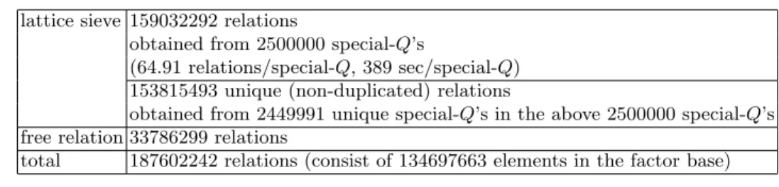
Table 3.Number of collected relations in collecting relations phase
lattice sieve 159032292 relations
obtained from 2500000 special-Q’s
(64.91 relations/special-Q, 389 sec/special-Q) 153815493 unique (non-duplicated) relations
obtained from 2449991 unique special-Q’s in the above 2500000 special-Q’s free relation 33786299 relations
total 187602242 relations (consist of 134697663 elements in the factor base)
5
Experimental results
We succeeded in solving a DLP overGF(36·97) by using the FFS with our efficient implementation techniques
discussed in Section 4. In this section, we report our computation results, such as the computational time of each phase of the FFS and the number of relations.
5.1 Polynomial Selection:
The FFS has six parameters κ, dH, dm, B, R,and S, as defined in Section 2.2, and we set (κ, dH, dm, B, R, S) = (3,6,33,6,6,6) for our target problem, based on the reason given in Section 3.2. In the polynomial selection phase, we can extract appropriate polynomials such as the definition polynomial H(x, y) of a function field described in Section 3.2 in one minute, so the computational cost of the polynomial selection phase is negligibly small.
5.2 Collecting relations phase
In the collecting relations phase, we search many relations that are equations of the form (8) to generate a system of linear equations by using the lattice sieve and the free relation. We explain our computational results of the collecting relations phase, e.g., the number of relations obtained in this phase, the computational time of the lattice sieve for one special-Q.
Lattice sieve: Each special-Qhas to be chosen fromFR(6)\FR(5). The number of elements ofFR(6)\FR(5) is 64563408, and the size of the table of those elements is about 500 MB. Since our program of the lattice sieve is computed using many nodes, it is not convenient to pick up the element from that 500-MB table as a special-Q. Therefore, we selected a special-Qby randomly generating an irreducible polynomial inGF(33)[x] of degree 6, which is inFR(6)\FR(5), and iterated the computation of the lattice sieve for the special-Q.
We prepared 47 PCs (in total 212 CPU cores) of (a)-(c) and (e)-(g) in Table 9 in Appendix C for the lattice sieve. The computation of the lattice sieve began on May 14, 2011, and we continued optimizing our program of the collecting relations phase. Figure 1 shows the process of our improvements in the collecting relations phase for the first two weeks. The total time for the collection of relations shortened due to our improvements. In the center of Fig. 1, there is a period in which no relations were obtained, from 8.5 to 9.4 days. This was due to human error; therefore, we wasted computer power during one day since a set of “seeds” to compute the program for each PC had been exhausted in the server PC during this period. As discussed in Section 4.1, we applied several improvements to our program of the collecting relations phase; lattice sieve for JL06-FFS, the lattice sieve with SIMD, and optimization for our parameters. Finally, as Table 8 in Appendix C shows, the computation finished on September 9, 2011 and required 118 days including the loss-time of some programming errors, updating our codes, and power outages. The real computational time of the lattice sieve was equivalent to 53.1 days using 212 CPU cores such as Xeon E5440.
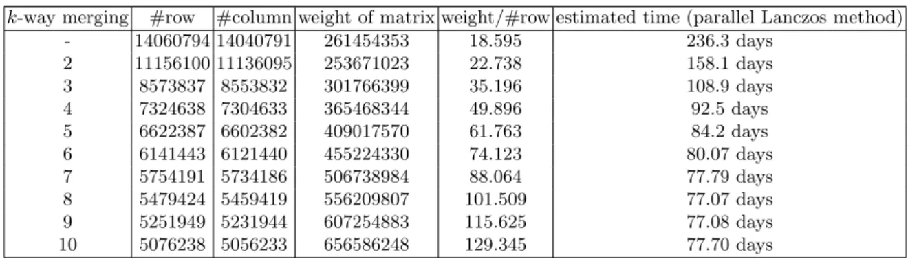
Table 4.Compressing matrix using Galois action, singleton-clique and merging
method size of matrix
before compressing 187602242 equations×134697663 variables Galois action 159394665 equations×45049572 variables singleton-clique 14060794 equations×14040791 variables 6-way merging 6141443 equations×6121440 variables
Table 5.Matrices after merging and computational time of parallel Lanczos method for matrices
k-way merging #row #column weight of matrix weight/#row estimated time (parallel Lanczos method) - 14060794 14040791 261454353 18.595 236.3 days
2 11156100 11136095 253671023 22.738 158.1 days 3 8573837 8553832 301766399 35.196 108.9 days 4 7324638 7304633 365468344 49.896 92.5 days 5 6622387 6602382 409017570 61.763 84.2 days 6 6141443 6121440 455224330 74.123 80.07 days 7 5754191 5734186 506738984 88.064 77.79 days 8 5479424 5459419 556209807 101.509 77.07 days 9 5251949 5231944 607254883 115.625 77.08 days 10 5076238 5056233 656586248 129.345 77.70 days
Free relation: The free relation gives us additional relations not generated by a sieving algorithm such as the lattice sieve. The details of the free relation is given in [19]. As shown in the sixth row in the right column in Table 3, the free relation gave us 33786299 relations. The seventh row in the right column in Table 3 means that we obtained 187602242 relations in total by adding relations given by the free relation to those generated using the lattice sieve. Eventually, we obtained a system of linear equations consisting of 187602242 equations and 134697663 variables. Note that there are 451002 elements in the factor base, which does not appear in the 187602242 relations
5.3 Linear algebra phase
Galois action : As mentioned in Section 4.2, the Galois action reduced the size of the matrix generated in the collecting relations phase to one-third sinceκ= 3. In fact, as the third row in the right column in Table 4 shows, the number of variables was reduced from 134697663 to 45049572, and the number of equations decreased from 187602242 to 159394665. This implies that the Galois action is appropriate for reducing variables of the matrix. To allay the fact that the size of each element of the matrix increases from a few bits to 151 bits due to the Galois action, we used theτ-adic structure mentioned in Section 4.2.
Singleton-clique : After using the Galois action, we additionally reduce the variables and equations of the matrix by singleton-clique [15]. To positively obtain the solutions of the system of linear equations in the linear algebra phase, we performed singleton-clique while keeping the number of variables larger than that of the equations by 20000. Therefore, as the fourth row in the right column of Table 4 shows, we obtained the matrix consisting of 14060794 rows and 14040791 columns. This computation takes 3 hours with a PC of (e) in Table 9 in Appendix C.
Table 6.Computational time of parallel Lanczos method for matrix reduced by 6-way merging
calculation time/loop 626.3 msec synchronization time/loop 46.5 msec communication time/loop 457.3 msec total time/loop 1130.1 msec number of loops 6121438 total time of parallel
80.1 days Lanczos method
Lanczos method for the 6-way merged matrix. After that, we had an opportunity to use a workstation that had 128-GB RAM and performed 7- to 10-way merging on the workstation. Eventually, we noticed that the computational cost of the Lanczos method for the 8-way merged matrix was three days less than that for 6-way merging. However, by this time, the computation of the parallel Lanczos method for the 6-way merged matrix had already been running for about seven days, so we continued computing the parallel Lanczos method for the 6-way merged matrix. The fifth row in the right column of Table 4 means that the 6-way merged matrix consisted of 6121440 variables and 6141443 equations. The entire computation for our merging took about 10 hours.
Parallel Lanczos method : We used the parallel Lanczos method [4, 19] to solve the system of linear equations defined by the 6-way merged matrix. Note that this matrix is sparse and defined overZP151, whereP151 is the
151-bit prime number given in Section 3.1. The computation of the parallel Lanczos method started on January 16, 2012, and was conducted on 21 PCs (in total 252 CPU cores) of (h) in Table 9 in Appendix C, which were connected via a 48-port Gbit HUB. As mentioned in Section 4.2, we continued improving our codes of the parallel Lanczos method after computation began. The computational times of our improved codes of the parallel Lanczos method are listed in Table 6. The number of loops of this method is equal to the rank of the 6-way merged matrix, and was at most 6121440. The computation for one loop required 626.3 msec on average. Additionally, for one loop, the synchronization time for communication among nodes was 46.5 msec on average, and the communication time for exchanging data among nodes was 457.3 msec on average. Therefore, the average time for one loop was 1130.1 msec. Finally, computation finished on April 14, 2012. The number of loops was 6121438 and the computation for the parallel Lanczos method took 90 days including time losses similar to our implementation of the lattice sieve. The real computational time is equivalent to 80.1 days using 252 CPU cores such as Xeon X5650.
5.4 Individual logarithm phase
Our target is to compute the discrete logarithm logg(ηT(Qπ,Qe)) and logg(ηT(Qπ,Qπ)) for someg ∈ G2, as
mentioned in Section 3.1.
Rationalization: Letgbe a polynomial (x+ω)(36·97−1)/P151 ∈G
2, whereω is a polynomial basis ofGF(33)∼= GF(3)[ω]/(ω3−ω−1). Note thatgis a generator ofG
2⊂GF(36·97)∗andx+ωis a monic irreducible polynomial
inFR(B) of degree 1. We search a pair (z1, z2) (and (z1′, z2′))∈(GF(33)[x])2such thatηT(Qπ,Qe)·gγ1 =z1/z2
(andηT(Qπ,Qπ)·gγ2 =z1′/z′2), wherezi(andz′i) areMi-smooth for someγ1, γ2∈ZP151 andi= 1,2. To reduce
the computational time of the following special-Qdescent, we tried to find as small anMi as possible within our computational resources fori= 1,2. In fact, we foundz1 andz2, which are 13- and 15-smooth (andz1′ and z′2which are 15- and 14-smooth), respectively. These computations were conducted on 168 CPU cores (PCs of (a)-(d) in Table 9 in Appendix C) and required 7 days for each computation.
ηT(Qπ,Qe)·gγ1 = (13-smooth)/(15-smooth)
γ1= 2514037766787322013334785428291787565870435706 ηT(Qπ,Qπ)·gγ2 = (15-smooth)/(14-smooth)
γ2= 2657516740789758289434702436228062607247517136
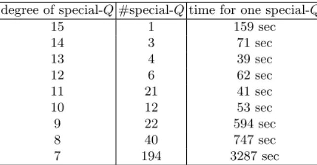
Table 7.Computational time for special-Qdescent in individual logarithm phase
degree of special-Q#special-Qtime for one special-Q
15 1 159 sec
14 3 71 sec
13 4 39 sec
12 6 62 sec
11 21 41 sec
10 12 53 sec
9 22 594 sec
8 40 747 sec
7 194 3287 sec
the number of irreducible factors in the computations of special-Qdescent and the time for computing them for each special-Q. These computations were conducted on 168 CPU cores (PCs of (a)-(d) in Table 9 in Appendix C) and took about 0.5 days in total. The computation for ηT(Qπ,Qπ) also took about 0.5 days in total on the same machine environment. Thus, as shown in Table 1, the computation of the individual logarithm phase took 15 days; 7 days (for rationalization)×2 elements + 0.5 days (for special-Qdescent)×2 elements.
By using the logarithms of the corresponding elements in the factor base obtained from the linear algebra phase, we could compute logg(ηT(Qπ,Qe)) and logg(ηT(Qπ,Qπ)). The logarithm of each element is as follows:
logg(ηT(Qπ,Qe)) = 1540966625957007958347823268423957036469656370,
logg(ηT(Qπ,Qπ)) = 1630281950635507295663809171217833096970449894.
Finally, we obtained the logarithm of the target element logη
T(Qπ,Qe)(ηT(Qπ,Qπ)) as follows:
logηT(Qπ,Qe)ηT(Qπ,Qπ) = 1752799584850668137730207306198131424550967300. (13) This is the solution of the ECDLP of equationQπ= [s]Qein (10). Scripts for checking this solution are provided in Appendix B.
6
Concluding remarks
We evaluated the security of pairing-based cryptosystems using theηT pairing over supersingular elliptic curves on finite fieldGF(3n). We focused on the case ofn= 97 since many implementers have reported practically rele-vant high-speed implementations of theηT pairing withn= 97 in both software and hardware. In particular, we examined the difficulty in solving the discrete logarithm problem (DLP) overGF(36·97) by our implementation of the function field sieve (FFS).
To reduce the computational cost of the FFS for solving the DLP over GF(36·97), we proposed several efficient implementation techniques. In the collecting relations phase, we implemented the lattice sieve for the JL06-FFS with SIMD and introduced improvements by optimizing for factor bases of each degree; therefore, our lattice sieve for the JL06-FFS became about 6 times faster than the first one. The main difference from the number field sieves for integer factorization is the linear algebra phase, namely, we have to deal with a large modulus of 151-bit prime for the computation of the FFS. We thus performed filtering (singleton-clique and merging) by carefully considering the data structure of large integers developing from the Galois action, so that we can efficiently conduct the parallel Lanczos method. From the above improvements, we succeeded in solving the DLP overGF(36·97) in 148.2 days by using PCs with 252 CPU cores. Our computational results contribute
to the security estimation of pairing-based cryptosystems using theηT pairing. In particular, they show that the security parameter of such pairing-based cryptosystems must be chosen withn >97.
Finally, we show a very rough estimation of required computational power for solving the DLP overGF(36n) withn >97. Our experiment on the DLP overGF(36n) withn= 97 used 252 CPU cores of mainly 2.67 GHz Xeon for 148.2 days, which are equivalent to 262.9 clock cycles. From the analysis of [30], the computational complexities of breaking the DLP overGF(36n) withn= 163 and 193 become 215.4and 219.1times larger than that withn= 97, respectively. Therefore, we could estimate that about 278.3and 282.0 clock cycles are required for breaking the DLP over GF(36n) with n = 163 and 193, respectively. On the other hand, the currently fastest supercomputer K has a throughput of about 10.5 petaflop/s from http://www.top500.org/, and it performs about 278.1 floating-point operations for one year. If one floating-point operation on the CPU of the
References
1. L. M. Adleman, “The function field sieve,” ANTS-I, LNCS 877, pp. 108-121, (1994).
2. L. M. Adleman and M.-D. A. Huang, “Function field sieve method for discrete logarithms over finite fields,” Inform. and Comput., Vol. 151, pp. 5-16, (1999).
3. O. Ahmadi, D. Hankerson, and A. Menezes, “Software implementation of arithmetic inF3m,” WAIFI 2007, LNCS 4547, pp. 85-102, (2007).
4. K. Aoki, T. Shimoyama, and H. Ueda, “Experiments on the linear algebra step in the number field sieve,” IWSEC 2007, LNCS 4752, pp. 58-73, (2007).
5. P. S. L. M. Barreto, S. Galbraith, C. ´O h ´Eigeartaigh, and M. Scott, “Efficient pairing computation on supersingular Abelian varieties,” Des., Codes Cryptogr., Vol. 42, No. 3, pp. 239-271, (2007).
6. P. S. L. M. Barreto, H. Y. Kim, B. Lynn, and M. Scott, “Efficient algorithms for pairing-based cryptosystems,” CRYPTO 2002, LNCS 2442, pp. 354-368, (2002).
7. J.-L. Beuchat, N. Brisebarre, J. Detrey, and E. Okamoto, “Arithmetic operators for pairing-based cryptography,” CHES 2007, LNCS 4727, pp. 239-255, (2007).
8. J.-L. Beuchat, N. Brisebarre, J. Detrey, E. Okamoto, M. Shirase, and T. Takagi, “Algorithms and arithmetic operators for computing theηT pairing in characteristic three,” IEEE Trans. Comput., Vol. 57, No. 11, pp. 1454-1468, (2008). 9. J.-L. Beuchat, N. Brisebarre, M. Shirase, T. Takagi, and E. Okamoto, “A coprocessor for the final exponentiation of
theηT pairing in characteristic three,” WAIFI 2007, LNCS 4547, pp. 25-39, (2007).
10. D. Boneh, G. Di Crescenzo, R. Ostrovsky, and G. Persiano, “Public key encryption with keyword search,” EURO-CRYPT 2004, LNCS 3027, pp. 506-522, (2004).
11. D. Boneh and M. Franklin, “Identity-based encryption from the Weil pairing,” CRYPTO 2001, LNCS 2139, pp. 213-229, (2001).
12. D. Boneh, C. Gentry, and B. Waters, “Collusion resistant broadcast encryption with short ciphertexts and private keys,” CRYPTO 2005, LNCS 3621, pp. 258-275, (2005).
13. D. Boneh, B. Lynn, and H. Shacham, “Short signatures from the Weil pairing,” ASIACRYPT 2001, LNCS 2248, pp. 514-532, (2001).
14. J. W. Bos, M. E. Kaihara, T. Kleinjung, A. K. Lenstra, and P. L. Montgomery, “Solving a 112-bit prime elliptic curve discrete logarithm problem on game consoles using sloppy reduction,” International Journal of Applied Cryptography, Vol. 2, No. 3, pp. 212-228, (2012).
15. S. Cavallar, “Strategies in filtering in the number field sieve,” ANTS-IV, LNCS 1838, pp. 209-231, (2000).
16. D. M. Gordon and K. S. McCurley, “Massively parallel computation of discrete logarithms,” CRYPTO’92, LNCS 740, pp. 312-323, (1992).
17. R. Granger, D. Page, and M. Stam, “Hardware and software normal basis arithmetic for pairing-based cryptography in characteristic three,” IEEE Trans. Comput., Vol. 54, No. 7, pp. 852-860, (2005).
18. D. Hankerson, A. Menezes, and M. Scott, “Software implementation of pairings,” Identity-Based Cryptography, pp. 188-206, (2009).
19. T. Hayashi, N. Shinohara, L. Wang, S. Matsuo, M. Shirase, and T. Takagi, “Solving a 676-bit discrete logarithm problem inGF(36n),” PKC 2010, LNCS 6056, pp. 351-367, (2010).
20. A. Joux, “A one round protocol for tripartite Diffie-Hellman,” ANTS-IV, LNCS 1838, pp. 385-394, (2000).
21. A. Jouxet al., “Discrete logarithms in GF(2607) andGF(2613),” Posting to the Number Theory List, available at http://listserv.nodak.edu/cgi-bin/wa.exe?A2=ind0509&L=nmbrthry&T=0&P=3690, (2005).
22. A. Joux and R. Lercier, “The function field sieve is quite special,” ANTS-V, LNCS 2369, pp. 431-445, (2002). 23. A. Joux and R. Lercier, “The function field sieve in the medium prime case,” EUROCRYPT 2006, LNCS 4004, pp.
254-270, (2006).
24. Y. Kawahara, K. Aoki, and T. Takagi, “Faster implementation ofηT pairing overGF(3m) using minimum number of logical instructions forGF(3)-addition,” Pairing 2008, LNCS 5209, pp. 282-296, (2008).
25. T. Kleinjung, K. Aoki, J. Franke, A. K. Lenstra, E. Thom´e, J. W. Bos, P. Gaudry, A. Kruppa, P. L. Montgomery, D. A. Osvik, H. J. J. te Riele, A. Timofeev, and P. Zimmermann, “Factorization of a 768-Bit RSA modulus,” CRYPTO 2010, LNCS 6223, pp. 333-350, (2010).
26. A. Menezes, T. Okamoto, and S. A. Vanstone, “Reducing elliptic curve logarithms to logarithms in a finite field,” IEEE Trans. IT, Vol. 39, No. 5, pp. 1639-1646, (1993).
27. T. Okamoto and K. Takashima, “Fully secure functional encryption with general relations from the decisional linear assumption,” CRYPTO 2010, LNCS 6223, pp.191-208, (2010).
28. J. M. Pollard, “The lattice sieve,” The development of the number field sieve, LNIM 1554, pp. 43-49, (1993). 29. A. Sahai and B. Waters, “Fuzzy identity-based encryption,” EUROCRYPT 2005, LNCS 3494, pp. 457-473, (2005). 30. N. Shinohara, T. Shimoyama, T. Hayashi, and T. Takagi, “Key length estimation of pairing-based cryptosystems
usingηT pairing,” ISPEC 2012, LNCS 7232, pp. 228-244, (2012).
A
Details of our implementation of collecting relations phase
Naive lattice sieve: First, we begin with the explanation of the naive lattice sieve for introducing notations. We define ¯FR(B) ={(p, t)|p∈FR(B), t≡m (modp)}and ¯FA(B) ={(p, t)| ⟨p, y−t⟩ ∈FA(B)}. In the lattice sieve, sieving is performed on (r, s)∈(GF(3κ)[x])2 such that rm+s(resp.r6x+s6 due toH(x, y) =x+y6) is divisible byq, where (q, u)∈F¯R(B) (resp. ¯FA(B)). This Q= (q, u) is called “special-Q”4. The (r, s) in the lattice sieve is represented asc(r1, s1) +d(r2, s2) forc, d ∈ GF(33)[x] of degree upper-bounded by C and D,
respectively, where (r1, s1),(r2, s2) are reduced lattice bases of (0, q),(1,−t), and sieving is performed on the
boundedc-dplane.
From among such pairs (r, s), we search a pair (c, d) such that rm+s (resp. r6x+s6) is divisible by p, where (p, t) ∈ SR ⊆F¯R(B) (resp.SA ⊆ F¯A(B)) is not equal to (q, u). We call sets SR and SA the rational sieving factor base and algebraic sieving factor base, respectively. The pair (c, d) is represented as (c0+kp, d)
fork∈GF(33)[x] and a fixedd, where
c0≡
{
−d(r1t+s1)−1(r2t+s2) (mod p) if (r1t+s1)̸≡0 (mod p)
any polynomials if (r1t+s1)≡0 andd≡0 (mod p)
This fact enables us to know which polynomial is the factor ofrm+s(resp.r6x+s6) without factoring these
polynomials. Thus, by computingc0+kp for a fixedd and each p∈SR (resp.SA), we can obtain (c, d) such thatrm+s(resp.r6x+s6) is divisible byp. For one (r, s) and a certain number of factorsp ofrm+s(resp. r6x+s6), if the sum of the degrees of all thepreaches a threshold, therm+s(resp.r6x+s6) isB-smooth with high probability. Such (r, s) is called a “candidate”. For each candidate, we determine whether it is aB-smooth pair by using the smoothness test [16].
In practice, a threshold is given by deg(rm+s)−ϵ(resp. deg(r6x+s6)−ϵ), whereϵis a non-negative integer,
called a “margin”. For a larger margin, we may obtain more relations but have to conduct additional smoothness tests. Conversely, for a smaller margin, we may lose some relations; however, the number of computations of the smoothness test decreases. Therefore, we should optimize the margin for efficient sieving.
A.1 SIMD implementation
In the lattice sieve, we treat elements inGF(33)[x] of the degree at most 6 since parameters B, R, andS are selected as 6, as mentioned in Section 3.2. As described in Section 4.1, we representGF(33) as polynomial basis
GF(3)[ω]/(ω3−ω−1) using 6-bit (h
1, ℓ1, hω, ℓω, hω2, ℓω2)∈GF(2)6. Then we can compute operations ofGF(3)
for coefficients ofωifori= 0,1,2 by logical instructions, as described in [24], so we can also compute operations ofGF(33) by logical instructions. In our implementation, we represent 16 elements inGF(33)[x] of degree at
most 7 using 6 registers of 128 bits, as shown in Fig. 2. Then we can compute an addition and a subtraction ofGF(33)[x] by logical instructions, and a multiplication byxand a division byxby shift instructions. These
operations are computed for 16 elements inGF(33)[x] with the SIMD.
A.2 Large prime variation
As shown in Table 2, the number of elements in the factor base of degree 6 is over 20 times larger than that of elements in the factor base of degree not larger than 5. Therefore, to compute the lattice sieve efficiently,
4
In Section 4.1, we defined special-QasQ∈FR(B), notQ∈F¯R(B) for simplicity.
128-bit register (8-bit×16 elements)
z }| {
8-bit
z }| {
· · · }h1
· · · }ℓ1
· · · }hω
· · · }ℓω
· · · }hω2
· · · }ℓω2
|{z}
x7
|{z}
x6
|{z}
x5
|{z}
x4
|{z}
x3
|{z}
x2
|{z}
x
|{z}
1
Note: an element inGF(33)∼=GF(3)[ω]/(ω3−ω−1) is represented using 6-bit (h
1, ℓ1, hω, ℓω, hω2, ℓω2)∈GF(2)6.

![Fig. 2. 128-bit data structure of 16 elements in GF (3 3 )[x] for SIMD implementation](https://thumb-us.123doks.com/thumbv2/123dok_us/7889203.1309120/15.892.180.728.929.1077/fig-bit-data-structure-elements-gf-simd-implementation.webp)
![Fig. 3. 128-bit data structure of element in GF (3 3 )[x] for smoothness test](https://thumb-us.123doks.com/thumbv2/123dok_us/7889203.1309120/16.892.176.729.935.1080/fig-bit-data-structure-element-gf-smoothness-test.webp)

