Fuzzy Sumudu Transform for Solving System of Linear Fuzzy Differential Equations with Fuzzy Constant Coefficients

Fuzzy Sumudu Transform for Solving System of

Linear Fuzzy Differential Equations with Fuzzy

Constant Coefficients

N.A. Abdul Rahman1,∗ ID_{, M.Z. Ahmad}2

1 _{School of Mathematical Sciences, Universiti Sains Malaysia, 11800 USM, Penang, Malaysia.;}

aswad.rahman@usm.my

2 _{Institute of Engineering Mathematics, Universiti Malaysia Perlis, Pauh Putra Main Campus, 02600 Arau,}

Perlis, Malaysia; mzaini@unimap.edu.my

* Correspondence: aswad.rahman@usm.my; Tel.: +604-6533944

Abstract: In this paper, we employ fuzzy Sumudu transform for solving system of linear fuzzy differential equations with fuzzy constant coefficients. The system with fuzzy constant coefficients is interpreted under strongly generalized differentiability. For this purpose, new procedures for solving the system are proposed. A numerical example is carried out for solving system adapted from fuzzy radioactive decay model. Conclusion is drawn in the last section and some potential research directions are given.

Keywords:fuzzy Sumudu transform; fuzzy linear differential equations; system of fuzzy differential equations

MSC:34A07, 65R10, 34A30

1. Introduction

For centuries, scientists have struggled to model real world phenomenon effectively and precisely. Among several modelling tools, scientists prefer to construct their models based on system of linear differential equations involving initial value problems [1–5]. This is because this kind of modelling are easier to be solved and analysed. However, the drawback of this modelling is very obvious and it is far from ideal. This is resulting from the lack of our knowledge about the world. Uncertainties or imprecisions occur in almost every aspect in our life, especially when dealing with real life phenomenon such as microbes, air and population. Using ordinary differential equations, the uncertainties are not dealt accordingly, thus, this leads to an inexact model.

To handle this shortcoming, scientist make use of Zadeh fuzzy set theory where the author emphasized that a number can be classified into certain membership function rather than we represent it as a discrete or crisp number [6]. The new modelling tool is referred to as fuzzy differential equations (FDEs). FDEs are developed whenever the structure of the model is non probabilistic. Unlike ordinary differential equations, FDEs take accounts the uncertainties or imprecisions observed circulating around the problem. There are a vast literature that can be found discussing FDEs as well as fuzzy derivatives [7–12].

So, the effort to construct methods for solving FDEs become an urgent matter. This includes both analytical and numerical methods. However, before we develop numerical methods for dealing with FDEs, it is important for us to construct analytical methods.

Recently, Ahmad and Abdul Rahman [13,14], proposed fuzzy Sumudu transform (FST) for solving FDEs with fuzzy initial values which was done under the strongly generalized differentiability concept. The authors successfully introduced some of FST fundamental properties and theories, and later demonstrated the proposed method on several numerical examples. As stated by the authors, the advantage of FST is significant as it reduces the complexity of the calculation when handling FDEs.

Plus, the final unit of the solution can be seen without even completing the solving process. This is due to its scale preserving property. Then, FST is used to solve fuzzy partial differential equations [15] before later, Haydar used FST to solve nth-order FDEs with fuzzy initial values [16]. The studies are the followed by the application of FST on fuzzy fractional differential equations and fuzzy Volterra integral equations in [17] and [18] respectively.

Scientists had continue utilizing FDEs to construct a more complex model which consists of several FDEs. The stepping stone for this effort is the development of system of linear first order fuzzy differential equations (SLFDEs). There has been several works regarding SLFDEs with fuzzy constant coefficients (FCCs) in the literature [19–24]. These include the implementation of variational iteration method and homotopy analysis method. When dealing with FDEs interpreted under strongly generalized differentiability concept, there are two cases of differentiability to be considered [11]. The previous works done did not demonstrated both cases efficiently, for example, the work in [19]. Particularly, only the first case is demonstrated by the authors. Because of this, we intend to use FST for solving SLFDEs with FCCs, and both cases of differentiability interpreted under the mentioned concept will be fully demonstrated. Plus, to the best of our knowledge, this is the first time FST is used to handle such system.

This paper is organized as follows. In Section 2, we recall several basic definitions and concepts of fuzzy numbers and fuzzy derivatives. In Section 3, we provide a general definition of FST. In addition, we also discuss on the scale preserving property possessed by FST and a brief comparison was done with fuzzy Laplace transform which has been proposed in [25]. Next in Section 4, we provide some details on the SLFDEs where two cases of the strongly generalized differentiability are considered. In Section 5, we construct detailed procedures to solve SLFDEs with FCCs. While in Section 6, a numerical example is demonstrated to show that the proposed method is practical. Later, in Section 7, we give conclusions.

2. Preliminaries

Several important definitions and properties for fuzzy numbers and fuzzy functions are recalled in this section. Note that the real number and fuzzy number are denoted byRandF(R), respectively,

throughout this paper.

Definition 1. [6] A fuzzy number is a mappingue:R→[0, 1]that satisfies the following conditions. 1. For everyue∈ F(R),u is upper semi continuous,e

2. for everyue∈ F(R),u is fuzzy convex, i.e.,e ue(γx+ (1−γ)y)≥min{ue(x),ue(y)}for all x,y∈R, and γ∈[0, 1],

3. for everyue∈ F(R),u is normal, i.e.,e ∃x0∈Rfor whichue(x0) =1,

4. suppue={x∈R|ue(x)>0}is the support ofu, and it has a compact closure cl(suppe u).e Definition 2. [26] Letue∈ F(R)andα∈]0, 1]. Theα-level set ofu is the crisp sete ue

α_{that contains all the}

elements with membership degree greater than or equal toα, i.e.

e

uα_={x∈

R|ue(x)≥α}, whereue

α_{denotesα-level set of fuzzy number}

e u.

It can be stated that theα-level of any fuzzy number is a bounded and closed set, and it is denoted by[uα_,uα_{], for both lower and upper bound of}

e

uα_{, respectively.}

Definition 3. [10,27] A parametric form of an arbitrary fuzzy numberu is an ordered paire [u

α_,uα_{]of functions}

uα_{and u}α_{, for anyα∈[0, 1], that fulfil the following conditions.}

2. uα_{is a bounded left continuous monotonic decreasing function in[0, 1],}

3. uα_≤uα_.

A fuzzy number is classified into certain membership function. In the literature, there are many types of membership function defined by researchers. For example, triangular, trapezoidal, Gaussian and generalized bell membership function. Among all of them, the triangular membership function is the most widely utilised by researchers. It is represented by three crisp numbers(a1,a2,a3)and its

α-level is computed as below [28].

e uα_{= [a}

1+ (a2−a3)α,a3−(a3−a2)α], α∈[0, 1]. (1) Basic operations between fuzzy numbers can be seen in [27].

Theorem 1. [29] Let the fuzzy function fe:R → F(R)represented by[fα(x),f

α

(x)]. For anyα∈ [0, 1], assume that fα_{(x)and f}α_{(x)are both Riemann-integrable on[a,b]and assume that there are two positive M}α

and MαwhereRb

a |fα(x)|dx≤Mαand

Rb

a |f α

(x)|dx≤ Mα, for every b ≥a. Then,fe(x)is improper fuzzy Riemann-integrable on[a,∞[and the improper fuzzy Riemann-integrable is a fuzzy number. Furthermore, we have

Z ∞

a

e

f(x)dx=

Z ∞

a f

α_(x)dx,

Z ∞

a f α

(x)dx

.

Definition 4. [9] Ifu,eve∈ F(R)and if there exists a fuzzy subsetξ∈ F(R)such thatξ+ue=v, thene ξis unique. In this case,ξis called the Hukuhara difference, or simply H-difference, of u and v and is denoted by e

v−H

e u.

The strongly generalized differentiability concept for a fuzzy function is described in the following definition.

Definition 5. [12,30] Let ef :]a,b[→ F(R)be a fuzzy function and x₀ ∈]a,b[. We say that ef is strongly generalized differentiable on x0, if there exists an elementfe0(x₀)∈ F(R), such that

1. for all h>0sufficiently small,∃ef(x₀+h)−H ef(x₀),ef(x₀)−H fe(x₀−h)and the limits (in the metric D)

lim

h→0

e

f(x0+h)−H ef(x₀) h =limh→0

e

f(x0)−H fe(x₀−h) h

= ef0(x₀),

or

2. for all h>0sufficiently small,∃ef(x₀)−H fe(x₀+h),ef(x₀−h)−H ef(x₀)and the limits (in the metric D)

lim

h→0

e

f(x0)−H ef(x₀+h) −h =limh→0

e

f(x0−h)−H ef(x₀) −h

= ef0(x₀).

Definition 6. [31] A fuzzy function ef : [a,b] → F(_R)is said to be continuous at x₀ ∈ [a,b] if for each e>0, there isδ>0such that D(fe(x),ef(x₀))<e, whenever x∈[a,b]and|x−x₀|<δ. We say that ef is continuous on[a,b]if ef is continuous at each x₀∈[a,b].

Theorem 2. [11] Let ef :R → F(R)be a continuous fuzzy function and ef(x) = [fα(x),f

α

(x)], for every α∈[0, 1]. Then

1. if the fuzzy function ef is (i)-differentiable, then fα(x)and f

α

(x)are both differentiable and

f0(x) = [(f0)α_(x),(f0₎α_(x)],

2. if the fuzzy function ef is (ii)-differentiable, then fα(x)and f

α

(x)are both differentiable and f0(x) = [(f0)α_(x),(f0₎α_(x)].

The next section provides the previously constructed FST. The concept for SLFDEs under the strongly generalized differentiability concept is also provided in this section.

3. Fuzzy Sumudu Transform

In order to construct the solution for SLFDEs, we adopted the Definition of FST introduced in [14].

Definition 7. [14] Let ef :_R→ F(_R)be a continuous fuzzy function. Suppose that ef(ux)e−xis improper fuzzy Riemann-integrable on[0,∞[, thenR∞

0 ef(ux)e−xdx is called fuzzy Sumudu transform and is denoted by

G(u) =S[ef(x)](u) = Z ∞

0

e

f(ux)e−xdx, u∈[−τ1,τ2],

where the variable u is used to factor the variable x in the argument of the fuzzy function andτ1,τ2>0.

FST can also be parametrically written as follows.

S[ef(x)](u) = [s[fα(x)](u),s[f

α

(x)](u)].

To explore theorems of FST, please see in [13,14]. In the following subsection, we provide a brief discussion on the scale preserving property of FST and for the sake of comparison, we introduce the time scaling property of fuzzy Laplace Transform. This is the first time such property of fuzzy Laplace transform is introduced in the literature, and it is mainly to compare how scaling effects both FST and fuzzy Laplace transform.

3.1. Discussion on Scale Preserving Property

One of the most frequently highlighted property of FST is the scale preserving property. The theorems for scale preserving are as follows.

Theorem 3. [14](First preserving Theorem) Let f :R→ F(R)be a continuous fuzzy-valued function and

a is an arbitrary constant, then

S[f(at)] =G(au).

Theorem 4. [14](Second preserving Theorem) Let f :R→ F(R)be a continuous fuzzy-valued function,

then

S

td f(t) dt

The theorems listed are the first and second preserving Theorem, respectively. From the scale preserving Theorems, it can be said that FST may be used to solve problems without resorting to a new frequency domain. Unlike other integral transforms, the integral transforms need to be resorted to a new domain before they can be solved. For example, fuzzy Laplace transform, where its time scaling is given by the following theorem.

Theorem 5. Let f :R→ F(R)be a continuous fuzzy-valued function and a is an arbitrary constant, then

L[f(at)] = 1

|a|F( s a), whereLis the fuzzy Laplace transform introduced in [25].

Proof. From [25], the parametric form of fuzzy Laplace transform is given as follows. L[f(at)] = [l[f(at)],l[f(at)]],

=

Z ∞

0 fα(at)e

−st_dt,Z ∞

0 fα(at)e

−st_dt.

We letm=at, so,dm

a =dt. Then, we have L[f(at)] =

Z ∞

0 fα(m)e

−s(m/a)dm

a , Z ∞

0 fα(m)e

−s(m/a)dm

a

,

= 1

a Z ∞

0 fα(m)e

−m(s/a)_dm,Z ∞

0 fα

(m)e−m(s/a)dm

.

By the definition of fuzzy Laplace transform, finally,

L[f(at)] = 1

aF( s a).

From Theorems3,4and5, we can see that, the scale is preserved when we apply FST to the original function but not when we apply fuzzy Laplace transform. This property of FST made it possible for researchers to treat the transformed function as a replica to the original function. In addition, this property also allows researchers to obtain the unit of the final solution even without transforming it back to the original domain. Such virtue is important for validation of the final results when complex systems are encountered.

4. System of First Order Linear Fuzzy Differential Equations

In this part, we consider the following linear system that has been presented in several papers previously [11,26,32]. Based on the papers, the FDEs are in a system of ordinary differential equations. Additionally, in this paper, the system are extended to two cases, in the sense of differentiability as in Definition5.

e

X0(t) =AeXe(t)⊕ef(t), (2) subjects to the initial conditions

e

X(0) =Xe0, (3)

where the constant coefficients areA,Xe(t) = [X₁(t),X₂(t), . . . ,Xn(t)]T,ef(t) = [f₁(t),f₂(t), . . . ,fn(t)]T, e

Let[Xm(t)]α= [(Xm)α(t),(Xm)α(t)],m=1, 2, . . . ,n, ifXm(t)is (i)-differentiable, then[X0m(t)]α= [(X0_m)α_(t),(X0

m)α(t)]. This is resulting from Theorem2. Thus form=1, 2, . . . ,n, we have (X0m)α(t) =

n

∑

j=1

aα

mj(Xj)α(t) + (f_m)α(t), (Xm)α(0) = (Xm0)α,

(X0m)α(t) = n

∑

j=1

aα

mj(Xj)α(t) + (fm)α(t), (Xm)α(0) = (Xm0)α,

(4)

and ifXm(t)is (ii)-differentiable, we have[X0m(t)]α = [(X 0

m)α(t),(X0m)α(t)]. So,

(X0m)α(t) = n

∑

j=1

aα

mj(Xj)α(t) + (f_m)α(t), (Xm)α(0) = (Xm0)α,

(X0_m)α_{(t) =} n

∑

j=1

aα

mj(Xj)α(t) + (fm)α(t), (Xm)α(0) = (Xm0)α,

(5)

where

aα

mj(Xj)α(t) =min{AX|A∈[(amj)α,(amj)α],X∈[(Xj)α(t),(Xj)α(t)]},

aα

mj(Xj)α(t) =max{AX|A∈[(amj)α,(amj)α],X∈[(Xj)α(t),(Xj)α(t)]}.

(6)

Consequently, ifXm(t)is (i)-differentiable, Eq. (4) is interpreted as the following.

1. Ifamjis non negative,

(X0_m)α_{(t) =} n

∑

j=1

(a_mj)α_(X

j)α(t) + (f_m)α(t), (X_m)α_{(0) = (X}

m0)α,

(X0m)α(t) = n

∑

j=1

(amj)α(Xj)α(t) + (fm)α(t),

(Xm)α_{(0) = (X} m0)α,

(7)

2. ifamjis non positive,

(X0_m)α_{(t) =} n

∑

j=1

(a_mj)α_(X

j)α(t) + (f_m)α(t), (X_m)α_{(0) = (X}

m0)α,

(X0m)α(t) = n

∑

j=1

(amj)α(Xj)α(t) + (fm)α(t), (Xm)α(0) = (Xm0)α.

(8)

1. Ifamjis non negative,

(X0m)α(t) = n

∑

j=1

(amj)α(Xj)α(t) + (f_m)α(t), (Xm)α(0) = (Xm0)α,

(X0m)α(t) = n

∑

j=1

(amj)α(Xj)α(t) + (fm)α(t), (Xm)α(0) = (Xm0)α,

(9)

2. ifamjis non positive,

(X0m)α(t) = n

∑

j=1

(amj)α(Xj)α(t) + (f_m)α(t), (Xm)α(0) = (Xm0)α,

(X0m)α(t) = n

∑

j=1

(amj)α(Xj)α(t) + (fm)α(t), (Xm)α(0) = (Xm0)α.

(10)

5. Fuzzy Sumudu Transform for System of Linear First Order Fuzzy Differential Equations Consider the following SLFDEs [26].

e

X0(t) =AeXe(t)⊕ef(t), (11) subjects to the initial conditions

e

X(0) =Xe0. (12)

Eq. (11) can also be rewritten as

e X0₁=

n

∑

j=1

ea1jXej(t) +fe1(t),

e X0₂=

n

∑

j=1

ea2jXej(t) +fe2(t), ..

.

e X0n =

n

∑

j=1

eanjXej(t) +fen(t),

(13)

or simply,

e Xm0 =

n

∑

j=1

eamjXej(t) + efm(t), (14) form=1, 2, . . . ,n, subjects to initial conditionsXe₀= [X₁₀,X₂₀, . . . ,X_n0]. By using FST on both sides of Eq. (14), we have

S[Xe 0

m](u) =S

" _n

∑

j=1

e

amjXe_j(t) +efm(t) #

(u). (15)

haveXe 0 m= [X

0 m,X

0

m]. IfXemis (ii)-differentiable, we haveXe 0 m= [X

0 m,X

0 m].

By Theorem 3.1 in [13], ifXemis (i)-differentiable, we have

S[Xe 0 m](u) =

G(u)−H

e Xm(0)

u ,

and this means that,

s " _n

∑

j=1

aα

mj(Xj)α(t) + (f_m)α(t)

#

(u) = s[(Xm)

α_(t)](u)−(X m)α(0)

u ,

s " _n

∑

j=1

aα

mj(Xj)α(t) + (fm)α(t)

#

(u) = s[(Xm)

α_(t)](u)−(X m)α(0)

u ,

(16)

wherem=1, 2, . . . ,n.

Also by Theorem 3.1 in [13], ifXemis (ii)-differentiable, we have

S[Xem](u) =

−Xem(0)−H(−G(u))

u ,

and this means that,

s " _n

∑

j=1

aα

mj(Xj)α(t) + (f_m)α(t)

#

(u) = s[(Xm)

α_{(t)](u)−(Xm)}α₍₀₎

u ,

s " _n

∑

j=1

aα

mj(Xj)α(t) + (fm)α(t)

#

(u) = s[(Xm)

α_(t)](u)−(X m)α(0)

u ,

(17)

wherem=1, 2, . . . ,n.

To solve Eq. (16) or (17), we assume that

s[(Xm)α(t)](u) =Lαm(u),

s[(Xm)α(t)](u) =Umα(u),

(18)

whereLα

1(u),U1α(u),Lα2(u),U2α(u), . . . ,Lαn(u)andUnα(u)are the solutions of Eq. (16) or (17). Then, by

the inverse of FST, the final solutions are as the following.

(Xm)α(t) =s−1[Lαm(u)], (Xm)α(t) =s−1[Umα(u)].

(19)

6. Numerical Example

The developed procedures is then applied on a numerical example. This is meant to demonstrate the applicability of FST in solving SLFDEs with FCCs.

Example 1. The following model is adapted from fuzzy radioactive decay model from [20]. In this model, r, N1,

N2,eλ₁andeλ2are considered to be triangular fuzzy numbers.

N₁0(t) =−eλ1N1(t) +r,

N20(t) =eλ₁N₁(t)−eλ₂N₂(t), N1(0) =N1, N2(0) =N2.

In [20], the authors stated that the values of r, N1, N2,eλ1andeλ2may be acquired from experts. The

lowest, the highest and the most exact values for r, N1, N2andeλ₁andeλ₂can be considered, and from this, five triangular fuzzy numbers are constructed. Their corresponding parametric representations can be calculated using Eq.(1). By using FST on both sides of Eq.(20),

S[N10(t)](u) =S[−λ1N1(t) +r](u),

S[N20(t)](u) =S[λ1N1(t)−λ2N2(t)](u).

(21)

This is equivalent to

S[N10(t)](u) =−λ1S[N1(t)](u) +r,

S[N20(t)](u) =λ1S[N1(t)](u)−λ2S[N2(t)](u).

(22)

Then, the procedures for solving Eq.(22)are divided into two cases. Case 1: First, consider both N1(t)and N2(t)to be (i)-differentiable. Then,

s[N1(t)](u)−N1(0)

u =−λ1s[N1(t)](u) +r, s[N1(t)](u)−N1(0)

u =−λ1s[N1(t)](u) +r, s[N2(t)](u)−N2(0)

u =λ1s[N1(t)](u)−λ2s[N2(t)](u), s[N2(t)](u)−N2(0)

u =λ1s[N1(t)](u)−λ2s[N2(t)](u).

(23)

Rearranging Eq.(23), it is obtained that

s[N₁(t)] +uλ1s[N1(t)](u) =N1(0) +ru,

s[N1(t)] +uλ1s[N1(t)](u) =N1(0) +ru,

s[N2(t)](u)−uλ1s[N1(t)](u) +uλ2s[N2(t)](u) =N2(0),

s[N2(t)](u)−uλ1s[N1(t)](u) +uλ2s[N2(t)](u) =N2(0).

(24)

Solving Eq.(24),

s[N1(t)](u) =(−λ1N1(0) +r)

u 1−λ₁λ1u2

−λ1r

u2

1−λ₁λ1u2

+N1(0)

1 1−λ₁λ1u2

,

s[N1(t)](u) =(−λ1N1(0) +r)

u 1−λ₁λ1u2

−λ₁r u

2

1−λ₁λ1u2

+N1(0) 1

1−λ₁λ1u2

,

s[N2(t)](u) =

1

(λ₁λ1u2−1)(λ₂λ2u2−1)

rλ1λ1λ2u4+N2(0) + (λ1λ1λ2N2(0) +λ₁λ1λ2N1(0)

−rλ1λ1−rλ2λ1)u3−(λ1λ1N2(0)−rλ1+N1(0)λ1λ1+N1(0)λ2λ1)u2−(λ2N2(0)

−N1(0)λ1)u),

s[N2(t)](u) =

1

(λ1λ₁u2−1)(λ2λ₂u2−1)

rλ1λ₁λ₂u4+N2(0) + (λ1λ₁λ₂N₂(0) +λ1λ₁λ₂N1(0)

−rλ1λ₁−rλ₂λ₁)u3−(λ1λ₁N2(0)−rλ1+N1(0)λ1λ₁+N₁(0)λ₂λ₁)u2−(λ₂N₂(0) −N1(0)λ1)u).

N1(t) =(−λ1N1(0) +r)q1 λ₁λ1

sinh(

q

λ₁λ1t) +N1(0)cosh(

q

λ₁λ1t)−λ1r



 cosh(

q

λ1λ1t)−1

λ₁λ1



,

N1(t) =(−λ1N1(0) +r)

1 q

λ₁λ1

sinh(

q

λ₁λ1t) +N1(0)cosh(

q

λ₁λ1t)−λ₁r 

 cosh(

q

λ1λ1t)−1

λ₁λ1



,

N2(t) =rλ1λ1λ2 e

−√λ1λ1t_(e2

√

λ1λ1t₊₁₎

2λ1λ1(λ₁λ1−λ₂λ2)

+e

−√λ2λ2t_(e2

√

λ2λ2t₊₁₎

2λ2λ2(λ₂λ2−λ₁λ1)

+ 1

λ₁λ1λ₂λ2

+N2(0)

λ₁λ1e−

√

λ1λ1t_(e2

√

λ1λ1t₊₁₎

2(λ₁λ1−λ₂λ2)

−λ2λ2e

−√λ2λ2t_(e2

√

λ2λ2t₊₁₎

2(λ₁λ1−λ₂λ2)

!

+ (λ₁λ1λ2N2(0)

+λ1λ1λ2N1(0)−rλ1λ1−rλ2λ1)



 e−

√

λ1λ1t_(e2

√

λ1λ1t₋₁₎

2 q

λ1λ1(λ1λ1−λ2λ2)

+e

−√λ2λ2t_(e2

√

λ2λ2t₋₁₎

2 q

λ2λ2(λ2λ2−λ1λ1)





−(λ1λ1N2(0)−rλ1+N1(0)λ1λ1+N1(0)λ2λ1)

e− √

λ1λ1t_(e2

√

λ1λ1t₊₁₎

2(λ₁λ1−λ₂λ2)

− e

−√λ2λ2t_(e2

√

λ2λ2t₊₁₎

2(λ₁λ1−λ₂λ2)

!

−(λ2N2(0)−N1(0)λ1)



 q

λ₁λ1e−

√

λ1λ1t_(e2

√

λ1λ1t₋₁₎

2(λ₁λ1−λ₂λ2)

− q

λ₂λ2e−

√

λ2λ2t_(e2

√

λ2λ2t₋₁₎

2(λ₁λ1−λ₂λ2)



,

N2(t) =rλ1λ1λ₂ e

−√λ1λ1t_(e2

√

λ1λ1t₊₁₎

2λ1λ1(λ₁λ1−λ₂λ2)

+e

−√λ2λ2t_(e2

√

λ2λ2t₊₁₎

2λ2λ2(λ₂λ2−λ₁λ1)

+ 1

λ₁λ1λ₂λ2

+N2(0)

λ₁λ1e−

√

λ1λ1t_(e2

√

λ1λ1t₊₁₎

2(λ₁λ1−λ₂λ2)

−λ2λ2e

−√λ2λ2t_(e2

√

λ2λ2t₊₁₎

2(λ₁λ1−λ₂λ2)

!

+ (λ₁λ1λ₂N₂(0)

+λ₁λ1λ₂N1(0)−rλ1λ1−rλ2λ1)



 e−

√

λ1λ1t_(e2

√

λ1λ1t₋₁₎

2 q

λ₁λ1(λ₁λ1−λ₂λ2)

+e

−√λ2λ2t_(e2

√

λ2λ2t₋₁₎

2 q

λ₂λ2(λ₂λ2−λ₁λ1)





−(λ1λ1N2(0)−rλ1+N1(0)λ1λ1+N1(0)λ2λ1)

e− √

λ1λ1t_(e2

√

λ1λ1t₊₁₎

2(λ₁λ1−λ₂λ2)

−e

−√λ2λ2t_(e2

√

λ2λ2t₊₁₎

2(λ₁λ1−λ₂λ2)

!

−(λ₂N₂(0)−N1(0)λ1)



 q

λ₁λ1e−

√

λ1λ1t_(e2

√

λ1λ1t₋₁₎

2(λ₁λ1−λ₂λ2)

− q

λ₂λ2e−

√

λ2λ2t_(e2

√

λ2λ2t₋₁₎

2(λ₁λ1−λ₂λ2)



.

Remark 1. The results in Case 1 are similar to results obtained by the authors in [19] and [33]. However, the authors in [19] and [33] only considered the condition when both N1(t)and N2(t)are (i)-differentiable. To the

best of our knowledge, this is the first time the solution for Case 2 (N1(t)and N2(t)to be (ii)-differentiable) for

Case 2: Next, consider that both N1(t)and N2(t)to be (ii)-differentiable. So,

s[N₁(t)]−N₁(0)

u =−λ1s[N1(t)] +r, s[N1(t)]−N1(0)

u =−λ1s[N1(t)] +r, s[N₂(t)]−N₂(0)

u =λ1s[N1(t)]−λ2s[N2(t)], s[N2(t)]−N2(0)

u =λ1s[N1(t)]−λ2s[N2(t)].

(25)

Rearranging Eq.(25),

(1+λ₁u)s[N₁(t)] =N₁(0) +ru,

(1+λ1u)s[N1(t)] =N1(0) +ru,

(1+λ₂u)s[N₂(t)]−λ1s[N1(t)]u=N2(0),

(1+λ2u)s[N2(t)]−λ₁s[N₁(t)]u=N2(0).

(26)

Solving Eq.(26),

s[N1(t)] =N1(0)

1

(1+λ₁u)+r u

(1+λ₁u), s[N1(t)] =N1(0) 1

(1+λ1u)

+r u

(1+λ1u)

,

s[N2(t)] =rλ1 u 2

(1+uλ1)(1+uλ2)

+N2(0)

1 1+uλ2

+N1(0)λ1 u

(1+uλ1)(1+uλ2)

,

s[N2(t)] =rλ1

u2

(1+uλ1)(1+uλ2)

+N2(0) 1

1+uλ2

+N1(0)λ1 u

(1+uλ1)(1+uλ2)

.

(27)

By using the inverse of FST, the solutions obtained are as follows.

N1(t) =N1(0)e−λ1t+r

1−e−λ1t

λ₁ , N1(t) =N1(0)e−λ1t+r1

−e−λ1t

λ1

,

N2(t) =rλ1 1

λ2−λ1

1−e−λ1t

λ1

−1−e

−λ2t

λ₂ !

+N1(0)λ1 1

λ2−λ1

(e−λ1t_−e−λ2t_{) +N}

2(0)e−λ2t,

N2(t) =rλ1

1

λ2−λ₁

1−e−λ1t

λ1

−1−e

−λ2t

λ2

!

+N1(0)λ1

1

λ2−λ₁

(e−λ1t_−e−λ2t_{) +N}

2(0)e−λ2t.

(28)

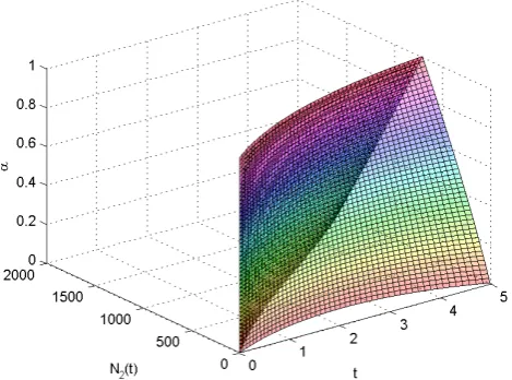
For illustration in tables and graphs, we let r= (4.9, 5, 5.1), N1 = (995, 1000, 1005), N2= (0, 0, 0),

e

λ1= (0.2, 0.3, 0.4)andeλ₂= (0.02, 0.03, 0.04)respectively. Their parametric representations can be calculated as in Definition1. The results of N1(t)and N2(t)for Case 1 are illustrated in Figs. 1and2, plotted using

MATLAB 2017 software, and the values are listed in Tables1and2. The results of N1(t)and N2(t)for Case 2

are illustrated in Figs.3and4, also using MATLAB 2017 software. The numerical values corresponding to this case are in Tables3and4.

For the sake of comparison, we would like to emphasized that the results obtained whenα=1are similar to the solutions for system of ordinary differential equations. Thus, it can be concluded that SLFDE is an extension of the system of ordinary differential equations. Furthermore, we can also said that SLFDE is a generalized version of system of ordinary differential equations since the set of real numbersRare subset of the set of fuzzy

numbers or fuzzy real numbersF(_R)The advantage of the solutions that we provided in this paper, is that this system are able to cope with uncertainties at initial values as well as having FCCs. This is very common when dealing with real life problems.

Figure 1.The graphical solution ofN1(t)in Eq. (20) for Case 1.

7. Conclusions

In this work, we have studied FST for solving SLFDEs with FCCs. One of the advantage of FST, the scale preserving property has been highlighted in Subsection3.1. This is done to justify why we chose to utilize FST in this paper. Then, procedures for obtaining the solutions of SLFDEs using FST are constructed in Section5. The process for finding the solutions is then demonstrated on a numerical

Figure 3.The graphical solution ofN1(t)in Eq. (20) for Case 2.

Figure 4.The graphical solution ofN2(t)in Eq. (20) for Case 2.

Table 1.The solutions ofN1(t)in Eq. (20) for Case 1.

α t=0.00 t=2.00 t=4.00

Table 2.The solutions ofN2(t)in Eq. (20) for Case 1.

α t=0.00 t=2.00 t=4.00

N₂(t) N2(t) N2(t) N2(t) N2(t) N2(t) 0.0 0.0000 0.0000 227.2468 682.1144 159.7583 1265.3728 0.1 0.0000 0.0000 246.7859 656.6515 202.8278 1202.1398 0.2 0.0000 0.0000 266.7095 631.4204 247.5739 1139.2478 0.3 0.0000 0.0000 287.0105 606.4306 293.9422 1076.7858 0.4 0.0000 0.0000 307.6815 581.6917 341.8578 1014.8416 0.5 0.0000 0.0000 328.7148 557.2130 391.3146 953.5020 0.6 0.0000 0.0000 350.1029 533.0038 442.1961 892.8524 0.7 0.0000 0.0000 371.8379 509.0733 494.4550 832.9766 0.8 0.0000 0.0000 393.9118 485.4305 548.0236 773.9570 0.9 0.0000 0.0000 416.3164 462.0842 602.8317 715.8741 1.0 0.0000 0.0000 439.0433 439.0433 658.8067 658.8067

Table 3.The solutions ofN1(t)in Eq. (20) for Case 2.

α t=−4.00 t=−2.00 t=0.00

N1(t) N1(t) N1(t) N1(t) N1(t) N1(t) 0.0 2183.2000 4929.4000 1471.8000 2221.7000 995.0000 1005.0000 0.1 2274.0000 4732.9000 1502.5000 2176.4000 995.5000 1004.5000 0.2 2368.7000 4544.3000 1533.7000 2132.1000 996.0000 1004.0000 0.3 2467.2000 4363.1000 1565.7000 2088.7000 996.5000 1003.5000 0.4 2569.9000 4189.2000 1598.2000 2046.1000 997.0000 1003.0000 0.5 2676.8000 4022.1000 1631.5000 2004.4000 997.5000 1002.5000 0.6 2788.1000 3861.7000 1665.4000 1963.6000 998.0000 1002.0000 0.7 2904.0000 3707.7000 1700.1000 1923.6000 998.5000 1001.5000 0.8 3024.8000 3559.8000 1735.5000 1884.4000 999.0000 1001.0000 0.9 3150.5000 3417.8000 1771.6000 1846.0000 999.5000 1000.5000 1.0 3281.4000 3281.4000 1808.4000 1808.4000 1000.0000 1000.0000

Table 4.The solutions ofN2(t)in Eq. (20) for Case 2.

α t

=−4.00 t=2.00 t=0.00

N2(t) N2(t) N2(t) N2(t) N2(t) N2(t) 0.0 4123.2773 1319.8732 1258.5979 510.5217 0.0000 0.0000 0.1 3925.9438 1415.0427 1213.9111 541.4794 0.0000 0.0000 0.2 3736.1399 1513.8730 1170.0869 573.0349 0.0000 0.0000 0.3 3553.5696 1616.5135 1127.1079 605.2005 0.0000 0.0000 0.4 3377.9487 1723.1200 1084.9570 637.9888 0.0000 0.0000 0.5 3209.0041 1833.8546 1043.6176 671.4126 0.0000 0.0000 0.6 3046.4736 1948.8858 1003.0733 705.4850 0.0000 0.0000 0.7 2890.1052 2068.3893 963.3081 740.2193 0.0000 0.0000 0.8 2739.6568 2192.5479 924.3062 775.6291 0.0000 0.0000 0.9 2594.8959 2321.5519 886.0523 811.7284 0.0000 0.0000 1.0 2455.5991 2455.5991 848.5313 848.5313 0.0000 0.0000

surrounded with fuzziness. For future research, we intend to explore other real life problems. Besides, we will also focus on integrating FST for solving system of fuzzy nonlinear problems.

8. Conflict of Interests

The authors declared that there is no conflict of interest.

Author Contributions:Conceptualization, N.A. Abdul Rahman and M.Z. Ahmad; Methodology, N.A. Abdul Rahman and M.Z. Ahmad; Validation, N.A. Abdul Rahman and M.Z. Ahmad; Writing—Original Draft Preparation, N.A. Abdul Rahman; Writing—Review & Editing,N.A. Abdul Rahman and M.Z. Ahmad; Visualization, N.A. Abdul Rahman

Acknowledgments:We would like to thank Universiti Sains Malaysia and Universiti Malaysia Perlis for providing facilities throughout this research.

Conflicts of Interest:The authors declare no conflict of interest.

Abbreviations

The following abbreviations are used in this manuscript:

FDE Fuzzy differential equation FST Fuzzy Sumudu transform

SLFDE System of linear fuzzy differential equation FCC Fuzzy constant coefficient

References

1. Guo, Y.; Wang, Y. Decay of dissipative equations and negative Sobolev spaces.Communications in Partial Differential Equations2012,37, 2165–2208.

2. Wang, M.; Zhang, Y. Two kinds of free boundary problems for the diffusive prey–predator model.Nonlinear Analysis: Real World Applications2015,24, 73–82.

3. Momani, S.; Odibat, Z. Numerical approach to differential equations of fractional order. Journal of Computational and Applied Mathematics2007,207, 96 – 110.

4. Caraballo, T.; Cheban, D. Almost periodic and almost automorphic solutions of linear differential/difference equations without Favard’s separation condition. I.Journal of Differential Equations 2009,246, 108 – 128.

5. Chirkunov, Y.A. Linear autonomy conditions for the basic Lie algebra of a system of linear differential equations. Doklady Mathematics2009,79, 415–417.

6. Zadeh, L.A. Fuzzy sets.Information and control1965,8, 338–353.

7. Chang, S.S.; Zadeh, L.A. On fuzzy mapping and control.IEEE Transactions on Systems, Man, and Cybernetics 1972, pp. 30–34.

8. Xu, J.; Liao, Z.; Hu, Z. A class of linear differential dynamical systems with fuzzy initial condition. Fuzzy Sets and Systems2007,158, 2339–2358.

9. Puri, M.L.; Ralescu, D.A. Differentials of fuzzy functions. Journal of Mathematical Analysis and Applications 1983,91, 552–558.

10. Ma, M.; Friedman, M.; Kandel, A. Numerical solutions of fuzzy differential equations. Fuzzy Sets and Systems1999,105, 133–138.

11. Chalco-Cano, Y.; Román-Flores, H. On new solutions of fuzzy differential equations. Chaos, Solitons & Fractals2008,38, 112–119.

12. Bede, B.; Rudas, I.J.; Bencsik, A.L. First order linear fuzzy differential equations under generalized differentiability.Information Sciences2007,177, 1648–1662.

13. Ahmad, M.Z.; Abdul Rahman, N.A. Explicit solution of fuzzy differential equations by mean of fuzzy Sumudu transform. International Journal of Applied Physics and Mathematics2015,5, 86–93.

14. Abdul Rahman, N.A.; Ahmad, M.Z. Applications of the fuzzy Sumudu transform for the solution of first order fuzzy differential equations. Entropy2015,17, 4582–4601.

16. Haydar, A.K. Fuzzy Sumudu transform for fuzzy nth-order derivative and solving fuzzy ordinary differential equations. International Journal of Science and Research2015,4, 1372–1378.

17. Abdul Rahman, N.A.; Ahmad, M.Z. Solving Fuzzy Fractional Differential Equations using Fuzzy Sumudu Transform.The Journal of Nonlinear Science and Applications2017,6, 19–28.

18. Abdul Rahman, N.A.; Ahmad, M.Z. Solving Fuzzy Volterra Integral Equations via Fuzzy Sumudu Transform.Applied Mathematics and Computational Intelligence2017,10, 2620–2632.

19. Fard, O.S.; Ghal-Eh, N. Numerical solutions for linear system of first-order fuzzy differential equations with fuzzy constant coefficients. Information Sciences2011,181, 4765 – 4779.

20. Gouyandeh, Z.; Armand, A. Numerical solutions of fuzzy linear system differential equations and application of a radioactivity decay model. Communications on Advanced Computational Science with Applications2013,2013, 1–11.

21. Allahviranloo, T. The Adomian decomposition method for fuzzy system of linear equations. Applied Mathematics and Computation2005,163, 553 – 563.

22. Khastan, A.; Nieto, J.J.; Rodríguez-López, R. Periodic boundary value problems for first-order linear differential equations with uncertainty under generalized differentiability. Information Sciences2013, 222, 544–558.

23. Mosleh, M. Fuzzy neural network for solving a system of fuzzy differential equations. Applied Soft Computing2013,13, 3597–3607.

24. Mosleh, M.; Otadi, M. Approximate solution of fuzzy differential equations under generalized differentiability.Applied Mathematical Modelling2015,39, 3003–3015.

25. Allahviranloo, T.; Ahmadi, M.B. Fuzzy Laplace transforms. Soft Computing2010,14, 235–243.

26. Kaleva, O. A note on fuzzy differential equations.Nonlinear Analysis: Theory, Methods & Applications2006, 64, 895–900.

27. Friedman, M.; Ma, M.; Kandel, A. Numerical solutions of fuzzy differential and integral equations. Fuzzy Sets and Systems1999,106, 35–48.

28. Kaufmann, A.; Gupta, M.M.Introduction to fuzzy arithmetic: Theory and applications; Van Nostrand Reinhold: New York, 1985.

29. Wu, H.C. The improper fuzzy Riemann integral and its numerical integration.Information Sciences1998, 111, 109–137.

30. Bede, B.; Gal, S.G. Generalizations of the differentiability of fuzzy-number-valued functions with applications to fuzzy differential equations. Fuzzy Sets and Systems2005,151, 581–599.

31. Guang-Quan, Z. Fuzzy continuous function and its properties. Fuzzy Sets and Systems1991,43, 159 – 171. 32. Allahviranloo, T.; Ahmady, N.; Ahmady, E. Numerical solution of fuzzy differential equations by

predictor–corrector method.Information sciences2007,177, 1633–1647.