www.astesj.com 66
Numerical Solution of Fuzzy Differential Equations with Z-numbers using Fuzzy Sumudu Transforms
Sina Razvarz1, Raheleh Jafari*,2, Wen Yu1
1Departamento de Control Automatico CINVESTAV-IPN (National Polytechnic Institute) Mexico City 07360, Mexico 2Department of Information and Communication Technology Agder University College, 4876 Grimstad, Norway
A R T I C L E I N F O A B S T R A C T
Article history:
Received: 14 November, 2017 Accepted: 17 January, 2017 Online: 30 January, 2018
The uncertain nonlinear systems can be modeled with fuzzy differential equations (FDEs) and the solutions of these equations are applied to analyze many engineering problems. However, it is very difficult to obtain solutions of FDEs.
In this paper, the solutions of FDEs are approximated by utilizing the fuzzy Sumudu transform (FST) method. Here, the uncertainties are in the sense of Z-numbers. Important theorems are laid down to illustrate the properties of FST. The theoretical analysis and simulation results show that this new technique is effective to estimate the solutions of FDEs.
Keywords:
K fuzzy Sumudu transform fuzzy differential equation Z-number
1. Introduction
This paper is an extension of work originally presented in [1]. In many physical and dynamical processes, mathematical modeling leads to the deterministic initial and boundary value problems. In practical the boundary values may be different from crisp and displays in the form of unknown parameters [2]. When the parameters or the states of the differential equations are uncertain, they can be modeled with FDE. In recent days, many methods have used FDE for modeling and control of uncertain nonlinear systems [3-5]. The basic idea of the fuzzy derivative was first introduced in [Chang]. Then it is extended in [6]. The first-order fuzzy initial value problem, as well as fuzzy partial differential equation, have been studied in [7]. By generalizing the differentiability, [6] gave an analytical solution. The Lipschitz condition, as well as the theorem for existence and uniqueness of the solution related to FDEs, are discussed in [10-12]. In [13], the analytical solutions of second order FDE are obtained. The analytical solutions of third order linear FDE are found in [14]. By the interval-valued method, [15] examined the basic solutions of nonlinear FDEs with generalized differentiability.
A novel technique in order to solve FDEs is laid down based on the Sumudu transform. Sumudu transform along with broad applications has been utilized in the area of system engineering and applied physics [16-18]. In [19], some simple and deeper fundamental theorems, as well as properties of the Sumudu
Transform, were generalized. In [20], Sumudu transform is applied to the system of differential equations. In [21], Sumudu transform is used in order to find the solution of the fuzzy partial differential equation. In [22], Sumudu transform has been used to solve fractional differential equations.
In this paper, we use FST to approximate the Z-number solutions of the FDEs. The FST reduces the FDE to an algebraic equation. A very important property of the FST is that it can solve the equation without resorting to a new frequency domain. The procedure of switching FDEs to an algebraic equation is cited in [10] and is stated as an operational calculus. We extend our previous work [1] by generating more theorems for describing the properties of FST and displaying the uncertainties with Z-numbers. The Z-number is a new concept that is subjected to a higher potential to demonstrate the information of the human being as well as to utilize in information processing [23]. Z-numbers can be regarded as to answer questions and carry out the decisions [24]. There exist few structure based on the theoretical concept of Z-numbers [25]. [26] gave an inception, which results in the extension of the Z-numbers. [27] generated a theorem to convert the Z-numbers to the usual fuzzy sets.
In this paper, initially, some preliminary definitions along with properties related to FST are demonstrated. After that, solving FDEs by using the methodology of FST has been discussed. At the end, two examples along with comparisons are utilized in order to demonstrate the effectiveness of our proposed method.
ASTESJ
ISSN: 2415-6698*Corresponding Author: Raheleh Jafari, [email protected]
www.astesj.com
Special issue on Advancement in Engineering Technology
2. Preliminaries
Prior to the introduction of the FST, some concepts related to the fuzzy variables and Z-numbers are laid down in this section [28, 29].
Definition 1: A fuzzy number 𝐵 is a function of
]
1
,
0
[
:
E
R
B
, in such a manner, 1) 𝐵 is normal, (there exists 𝑎0∈ 𝑅 in such a manner 𝐵(𝑎0) = 1; 2) 𝐵 is convex, 𝐵(𝛾𝑎 + (1 − 𝛾)𝑐) ≥ min{𝐵(𝑎), 𝐵(𝑐)},
a
,
c
R
,
[
0
,
1
]
; 3) 𝐵is upper semi-continuous on 𝑅 , i.e.,B
(
a
)
B
(
a
0)
,),
(
a
0N
a
a
0
R
,
0
,
N
(
a
0)
is a neighborhood; 4) The setB
{
a
R
,
B
(
a
)
0
}
is compact.Definition 2: The
r
-level of the fuzzy number 𝐵 is defined as follows}
)
(
:
{
]
[
B
r
a
R
B
a
r
(1)where
0
r
1
,B
E
.
Definition 3: Let
B
1,
B
2
E
and
R
, the operations addition, subtraction, multiplication and scalar multiplication are defined as]
,
[
]
[
]
[
]
[
1 2 1 2 1 2 1 2r r r r r r
r
B
B
B
B
B
B
B
B
(2)1 2
1 2
1 2 1 2
[
B B
?
]
r
[ ]
B
r
[
B
]
r
[
B
r
B B
r,
r
B
r]
(3)2 1 1 2
1 2 1 2
1 2
2 1 1 2
1 2 1 2
min{ , , , }
[ ? ]
max{ , , , }
r r r r
r r r r
r
r r r r
r r r r
B B B B B B B B
B B
B B B B B B B B
(4)
0
),
,
(
0
),
,
(
]
[
]
[
1 1
1 1 1
1
r r
r r r
r
B
B
B
B
B
B
(5)Definition 4: The Hausdorff distance between two fuzzy numbers
B
1 andB
2 is defined as [30,31]|)}
|
|,
(|
max
{
sup
)
,
(
1 2 1 21 0 2 1
r r r r
r
B
B
B
B
B
B
D
(6)
)
,
(
B
1B
2D
has the following properties(i)
D
(
B
1
u
,
B
2
u
)
D
(
B
1,
B
2),
B
1,
B
2,
u
E
(ii)
D
(
B
1,
B
2)
|
|
D
(
B
1,
B
2),
R
,
B
1,
B
2
E
(iii)
D
(
B
1
B
2,
u
v
)
D
(
B
1,
u
)
D
(
B
2,
v
),
E
v
u
B
B
1,
2,
,
(iv)
(
D
,
E
)
is stated as complete metric space.Definition 5: The function
:
[
a
1,
a
2]
E
is integrable on]
,
[
a
1a
2 , if it satisfies in the below mentioned relation)
)
,
(
,
)
,
(
(
)
(
1 1
1
dx
r
x
dx
r
x
dx
x
a a
a
(7)If
(
x
)
be a fuzzy value function, as well asq
(
x
)
be a fuzzy Riemann integrable on[
a
1,
]
so
(
x
)
q
(
x
)
can be a fuzzy Riemann integrable on[
a
1,
]
. Therefore,dx
x
q
dx
x
dx
x
q
x
a a
a1
(
(
)
(
))
(
)
(
)
(8)According to the fuzzy concept or in the case of interval arithmetic, equation
B
1
B
2
s
is not equivalent with1
?
2 1( 1)
2s
B B
B
B
or toB
2
B
1?
s
B
1
( 1)
s
and this is the main reason in introducing the following Hukuhara difference (H-difference).Definition 6: The definition of H-difference [32,9], is proposed by
B
1?
HB
2
s
B
1
B
2
s
. IfB
1?
HB
2 prevails, itsr
-level is[
1?
2]
[
1 2,
1 2]
r r
r r
r H
B
B
B
B B
B
.Precisely,
B
1?
HB
1
0
butB
1?
B
1
0
.Definition 7: Suppose
:[a1,a2]E andx
0
[
a
1,
a
2]
.
is strongly generalized differentiable atx
0,
if for allk
0
adequately minute,
(
x
0)
E
exists in such a manner that (i)
(
x
0
k
) ?
H
( )
x
0 ,
( ) ?
x
0 H
(
x
0
k
)
and0 0 0 0
( )? ( ) ( )? ( )
0 0
0
lim
lim
(
)
H H
x k x x x k
k k
k k
x
or (ii)
( ) ?
x
0 H
(
x
0
k
)
,
(
x
0
k
) ?
H
( )
x
0 and0 0 0 0
( )? ( ) ( )? ( )
( ) ( )
0 0
0
lim
lim
( ),
H H
x x k x k x
k k
k k
x
or (iii)
(
x
0
k
) ?
H
( )
x
0 ,
(
x
0
k
) ?
H
( )
x
0 and0 0 0 0
( )? ( ) ( )? ( )
( )
0 0
0
lim
lim
( )
H H
x k x x k x
k k
k k
x
or (iv)
( ) ?
x
0 H
(
x
0
k
)
,
( ) ?
x
0 H
(
x
0
k
)
and0 0 0 0
( )? ( ) ( )? ( )
( )
0 0
0
lim lim
( )
H H
x x k x x k
k k
k k
x
Remark 1:It is clear that case
(
i
)
is H-derivative. Furthermore, a function is (i)-differentiable only when it is H-derivative.Remark 2: It can be concluded from [32] that, the definition of differentiability is noncontradictory [33].
(i) If
be (i)-differentiable, so
(
t
,
r
)
and
(
t
,
r
)
aredifferentiable functions, moreover
(
t
)
(
(
t
,
r
),
(
t
,
r
))
. (ii) If
be (ii)-differentiable, so
(
t
,
r
)
and
(
t
,
r
)
aredifferentiable functions, moreover
(
t
)
(
(
t
,
r
),
(
t
,
r
))
. Suppose f :(a1,a2)R is differentiable on(
a
1,
a
2)
, furthermore
has finite root in (a1,a2) , andm
E
, therefore,) ( ) (x mf x
is strongly generalized differentiable on (a1,a2) along with
(
x
)
m
f
(
x
)
,
x
(
a
1,
a
2)
.Theorem 1: [9] Assume : REE is taken to be a continuous fuzzy function. If
x
0
R
, the fuzzy initial value constraint
0 0
)
(
)
,
(
)
(
x
x
t
(9)
is incorporated with two solutions: (i)-differentiable, also (ii)-differentiable. Hence the successive iterations
]
,
[
,
))
(
,
(
)
(
0 0 11
0
x
x
x
dt
t
t
x
x nx
n
(10)and
0
1
( )
0? ( 1)
( ,
( )) ,
[ , ]
0 1x
n
x
H xt
nt dt
x
x x
(11)approaches towards the two solutions sequentially.
Definition 8: A Z-number has two components Z
B(a),p~
. The primary component B(a) is restriction on a real-valueduncertain variable 𝑎. The secondary component
~
p
is a measure of the reliability of 𝐵. p~ can be reliability, the strength of belief, probability or possibility. When B(a) is a fuzzy number and ~p is the probability distribution of 𝑎, the Z-number is stated as 𝑍+-number. When
B
(
a
)
as well as~
p
are fuzzy numbers, the Z-number is stated as 𝑍− -number.The 𝑍+ -number carries more information when compared
with 𝑍− -number. In this paper, we utilize the definition of 𝑍+
-number, i.e., Z
B,~p, 𝐵 is a fuzzy number and ~ is a pprobability distribution.
To express the fuzzy number the most common membership functions are utilized in this paper. The popular membership functions are the triangular function
,
,
0
3 2
2 1
3 2 1
2 3 3
1 2
1
B a
B
otherwise
a
a
F
(12)
and trapezoidal function
01 ,
, ,
3 2
4 3
2 1
4 3 2
1 4 3
4 1 2
1
B a
a
B otherwise
a a a
F
(13)
The probability measure is defined as
da
a
p
a
P
BR
(
)
~
)
(
~
(14)where
~
p
is the probability density ofa
, also 𝑅 is the restriction on~
p
.
For discrete Z-numbers)
(
~
)
(
)
(
~
1
i i B n
i
a
p
a
B
P
(15)Definition 9: The
r
-level of the Z-numberZ
(
B
,
P
~
)
is illustrated as
r r
r
p
B
Z
]
[
]
,
[
~
]
[
(16)where
0
r
1
.[
p
~
]
r is computed by the Nguyen's theorem
r r r r rr
P
P
B
B
p
B
p
p
]
~
([
]
)
~
([
,
])
~
,
~
~
[
(17)where
~
p
([
B
]
r)
~
p
(
a
)
|
a
[
B
]
r
. So[
Z
]
r can be demonstrated as the formr
-level of a fuzzy number
r r r r r rr
P
B
P
B
Z
Z
Z
]
,
,
~
,
,
~
[
(18)where
P
~
r
B
rp
~
(
a
ir)
, ~ ~( ir)r r
a p B
P ,
[
]
(
,
ir).
r i r
i
a
a
a
Similar with the fuzzy numbers, the Z-numbers are also incorporated with three primary operations, addition, subtraction, and multiplication. The operations in this paper are different definitions with [34]. The
r
-level of Z-numbers is applied to simplify the operations.Suppose Z1(B1,~p1) and Z2 (B2,~p2) be two discrete
Z-numbers expressing the uncertain variables
a
1 anda
2,
,
1
)
(
~
1 1
1
np
a
1~
p
2(
a
2)
1
n . The operations are displayed
as
)
~
~
,
(
1 2 1 22 1
12
Z
Z
B
B
p
p
Z
(19)where
{ , ?, ?}
.For all
~
p
1
~
p
2 operations, we use convolutions for the discrete probability distributions
)
~
(
)
(
~
)
(
~
~
~
12 ,
2 2 , 1 1 2
1
p
p
a
p
a
p
a
p
i n ii
(20)The above definitions satisfy the Hukuhara difference [35],
1 2 12
1 2 12
?
HZ
Z
Z
Z
Z
Z
If
Z
1?
HZ
2 prevails, ther
-level is1 2
1 2
1 2
[
Z
?
HZ
]
r
[
Z
r
Z
r,
Z
r
Z
r]
(22)Obviously,
Z
1?
HZ
1
0
,Z
1?
Z
1
0
.Also the above definitions satisfy the generalized Hukuhara difference [7]
1 2 12
1 2 12
2 1 12
1)
?
2)
( 1)
gH
Z
Z
Z
Z
Z
Z
Z
Z
Z
(23)It is easy to display that 1) and 2) in combination are genuine if and only if
Z
12 is a crisp number. With respect tor
-level we have1 2 1 2
1 2 1 2
1 2
[ ? ]r [min{ r r, r r}, max{ r r, r r}]
gH
Z Z Z Z Z Z Z Z Z Z
and If Z1gHZ2 and Z1HZ2 subsist, Z1?HZ2Z1?gHZ2. The circumstances for the inerrancy of
12 1?gH 2
Z Z Z E are
12 1 2
12 1 2
12 12
12 12
1 2 12
12 1 2
12 12
12 12
1)
sin ,
sin ,
2)
sin ,
sin ,
r r r
r r r
r r
r r
r r r
r r r
r r
r r
Z
Z
Z and Z
Z
Z
with Z increa
g Z decrea
g Z
Z
Z
Z
Z and Z
Z
Z
with Z increa
g Z decrea
g Z
Z
(24)
where
r
[
0
,
1
]
If
B
is a triangular function, the absolute value of the Z-number) ~ , (B p
Z is defined as
|))
|
|
|
|
(|
~
|,
|
|
|
|
(|
)
(
a
11
12
13p
21
22
23Z
(25)If 𝐵1, as well as 𝐵2 are triangular functions, the supremum metric for 𝑍-numbers Z1(B1,~p1) and Z2 (B2,~p2) is illustrated as
)
~
,
~
(
)
,
(
)
,
(
Z
1Z
2d
B
1B
2d
p
1p
2D
(26)in this case
d
(
,
)
is defined as the supremum metrics with fuzzy sets [3].D
(
Z
1,
Z
2)
is incorporated with the following possessions)
,
(
)
,
(
)
,
(
)
,
(
|
|
)
,
(
)
,
(
)
,
(
)
,
(
)
,
(
2 1
2 1
2 1 2
1
2 1 1
2
2 1 2
1
Z
Z
D
Z
Z
D
Z
Z
D
Z
Z
D
Z
Z
D
Z
Z
D
Z
Z
D
Z
Z
D
Z
Z
Z
Z
D
where
R
, Z(B,~p) is Z-number and 𝐵 is triangle function, for proof refer to [36].Definition 10: Suppose
Z
ˆ
demonstrates the space of Z -numbers, then ther
level of Z -number valued functionZ
a
a
,
]
ˆ
[
:
1 2
is defined as)]
,
(
),
,
(
[
)
,
(
r
r
r
where
Z
ˆ
, and r[0,1] .Based on the definition of Generalized Hukuhara difference,
the gH-derivative of
at
0 is defined as0 0 0
0
1
(
)
lim [ (
) ?
gH(
)]
h
h
h
(27)In (27),
(
0
h
)
and
(
0)
represents similar style with 𝑍1and 𝑍2respectively defined in (laiop).
By implementing the 𝑟 − level (16) to initial value problem,
))
(
,
(
)
(
t
t
t
, we generate two Z-number valued functions:
t
,
(
a
,
r
),
(
a
,
r
)
and
t,
(a,r),
(a,r)
.The initial value problem can be equivalent to the following relation
)
,
(
),
,
(
,
)
,
(
),
,
(
,
)
)
,
(
),
,
(
,
)
,
(
),
,
(
,
)
r
a
r
a
t
r
a
r
a
t
ii
r
a
r
a
t
r
a
r
a
t
i
(28)
3. Fuzzy Sumudu transform
Fuzzy initial and boundary value problems can be resolved by utilizing fuzzy Laplace transform [10]. In this paper, the FST methodology for Z-number is illustrated, furthermore the properties of this methodology is stated. By applying the FST methodology, the FDE based on Z-number is reduced to an algebraic equation. The main advantage of the FST is that it can resolve the equation without resorting to a new frequency domain. The methodology of converting FDEs to an algebraic equation is expressed in [10].
Definition 11: Suppose
(
t
)
be a continuous Z-number valued function, also,(
) ?
tBt
e
be an improper Z-number
Riemann integrable on
[
0
,
)
. Accordingly,0 ( ) ?
t
Bt e dt
is
expressed as FST and it is defined by
0
( )B [ ( )] t (Bt) ?e dtt
S , where
0
B
K
,K
0
, also
e
t is a real-valued function. Based on the Theorem 3 we have the following relation0 ( ) ? ( 0 ( , ) , 0 ( , ) )
t t t
Bt e dt Bt r e dt Bt r e dt
(29)Let
0
0
[ ( , )]
(
, )
[ ( , )]
(
, )
t
t
t r
Bt r e dt
t r
Bt r e dt
S
S
(30)
hence we obtain the following relation
)])
,
(
),
,
(
[
(
)]
(
[
t
S
t
r
S
t
r
Theorem 2: Suppose
(
t
)
be a Z-number valued integrable function, as well as
(
t
)
be the primitive of
(
t
)
on[
0
,
)
. Therefore,1 1
[ ( )]t ? [ ( )]?(t ?[ (0)])
B B
S S (32)
where
is considered to be (i)-differentiable, or1
1
[
( )]
t
?[ (0)]?(
? [ ( )])
t
B
B
S
S
(33)where
is considered to be (ii)-differentiable.Proof. For arbitrary fixed
r
[
0
,
1
]
we have1 1
1 1 1 1
? [ ( )]?( ? (0))
(
[ ( , )]
[ (0, )],
[ ( , )]
[ (0, )])
B B
B B B B
t
t r
r
t r
r
S
S
S
S
S
(34)
We have the following relations
)]
,
0
(
[
)]
,
(
[
)]
,
(
[
)]
,
0
(
[
)]
,
(
[
)]
,
(
[
1 1
1 1
r
r
t
r
t
r
r
t
r
t
B B
B B
S
S
S
S
(35)
Hence, we obtain
1 1
? [ ( )]?(t ? (0)) ( [ ( , )], [t r ( , )])t r
B
B
S S S (36)
If
is considered to be (i)-differentiable, so1
1
? [ ( )]?(
t
? (0))
[
( )]
t
B
S
B
S
(37)Let
is (ii)-differentiable. For arbitrary fixed
[
0
,
1
]
weobtain
1 1
1 1 1 1
?[ (0)]?( ? [ ( )])
(
(0, )
[ ( , )],
(0, )
[ ( , )])
B B
B B B B
t
r
t r
r
t r
S
S
S
(38)
The above equation can be written as the following relation
1 1
1 1 1 1
?[ (0)]?( ? [ ( )])
( [ ( , )] (0, ), [ ( , )] (0, ))
B B
B B B B
t
t r r t r r
S
S S
(39)
We obtain
)
,
0
(
)]
,
(
[
)]
,
(
[
)
,
0
(
)]
,
(
[
)]
,
(
[
1 1
1 1
r
r
t
r
t
r
r
t
r
t
B B
B B
S
S
S
S
(40)
So, we have
1 1
( (0)) ?( ? [ ( )])t ( [ ( , )], [t r ( , )])t r
B
B
S S S (41)
Hence
1 1
( (0)) ?( ? [ ( )])t ([ ( , )],[t r ( , )])t r
B
B
S S (42)
Since
is (ii)-differentiable, therefore,1
1
(
(0)) ?(
? [ ( )])
t
[
( )]
t
B
B
S
S
(43)Theorem 3: Taking into consideration that Sumudu transform is a linear transformation, so if
(
t
)
and
(
t
)
be continuous Z-number valued functions, moreoverk
1 as well ask
2 be constant, therefore the following relation can be obtained1 2 1 2
[( ? ( ))k t (k ? ( ))]t ( ? [ ( )])k t (k ? [ ( )])t
S S S (44)
Proof. We have
1 2
1 2
0
1 2
0 0
1 0 2 0
1 2
[( ? ( )) ( ? ( ))]
( ? ( ) ? ( )) ?
? ( ) ? ? ( ) ?
?( ( ) ? ) ?( ( ) ? )
? [ ( )] ? [ ( )]
t
t t
t t
k t k t
k Bt k Bt e dt
k Bt e dt k Bt e dt
k Bt e dt k Bt e dt
k t k t
S
S S
(45)
Therefore, we conclude
1 2 1 2
[( ? ( ))k t (k ? ( ))]t ( ? [ ( )])k t (k ? [ ( )])t
S S S (46)
Lemma 1: Assume that
(t) is a continuous Z-number value function on[
0
,
)
, also
0
, thus[ ?
( )]
t
? [ ( )]
t
S
S
(47)Proof. Fuzzy Sumudu transform
? ( )
t
is defined as0
[ ? ( )]
t
? (
Bt
) ?
e dt
tS
(48)furthermore, we have
0
? (
) ?
?
0(
) ?
t t
Bt
e dt
Bt
e dt
(49)therefore,
[ ? ( )]t ? [ ( )] t
S S (50)
Lemma 2: Assume that
(
t
)
is a continuous Z-number valued function, and
(
t
)
0
. Furthermore, if we suppose that( ( ) ? ( )) ?
t
t
e
t is improper Z-number Reiman integrable on)
,
0
[
, then0
0 0
( (
) ? (
)) ?
(
(
) (
, )
,
(
) (
, )
)
tt t
Bt
Bt
e dt
Bt
Bt r e dt
Bt
Bt r e dt
(51)Theorem 4: Suppose (t) is a continuous Z-number valued function, also
S
[
(
t
)]
D
(
B
)
, therefore,1
1 1
1
[
? ( )]
(
)
1
1
a t
B
e
t
D
a B
a B
S
(52)where
e
a1t is considered to be a real value function, alsoProof. We have the following relation
1 1
1 1
0
(1 ) (1 )
0 0
[
? ( )]
(
)
(
(
, ) ,
(
, ) )
a t a Bt t
a B t a B t
e
t
e
e
Bt dt
e
Bt r dt
e
Bt r dt
S
(53)Let us consider
z
1
a
1Bt
, then1
1 1 1
1 1 1 1 1 1
1
1 0 1 0 1
1 1 1
1 1 1 1 1 1
[
? ( )]
(
(
, )
,
(
, )
)
{
(
),
(
)}
(
)
a t z z Bz Bza B a B a B
B B B
a B a B a B a B a B a B
e
t
r e dz
r e dz
D
D
D
S
(54)4. Solving fuzzy initial value problem with fuzzy Sumudu transform method
Consider the following fuzzy initial value problem based on Z-numbers
1
0
)),
,
0
(
),
,
0
(
(
)
0
(
)),
(
,
(
)
(
r
r
r
t
t
t
(55)where
(
t
,
(
t
))
is a Z-number function. By utilizing FST method for Z-numbers, we obtain))]
(
,
(
[
)]
(
[
t
S
t
t
S
(56)The solving process of Eq. (56) is based on the following cases.
Case 1: Assume that
(
t
)
is (i)-differentiable. Base on the Theorem 3 we extract))
,
(
),
,
(
(
)
(
t
t
r
t
r
(57)1
1
[ ( )]
t
(
? [ ( )]) ?
t
(0)
B
B
S
S
(58)Eq. (58) can be displayed as the following relation
)
,
0
(
)]
,
(
[
)]
),
(
,
(
[
)
,
0
(
)]
,
(
[
)]
),
(
,
(
[
1 1 1 1r
r
t
r
t
t
r
t
r
t
t
B B B B
S
S
S
S
(59) where
))}
,
(
),
,
(
(
|
)
,
(
max{
)
),
(
,
(
))}
,
(
),
,
(
(
|
)
,
(
min{
)
),
(
,
(
r
t
r
t
B
B
t
r
t
t
r
t
r
t
B
B
t
r
t
t
(60)Accordingly, Eq. (60) can be resolved on the basis of the following assumptions
)
,
(
)]
,
(
[
t
r
U
1B
r
S
(61))
,
(
)]
,
(
[
t
r
U
2B
r
S
(62)where U1(B,r) , as well as
U
2(
B
,
r
)
are the Z-number solutions of the Eq. (60). By applying inverse Sumudu transform,
(
t
,
r
)
as well as
(
t
,
r
)
are computed as)]
,
(
[
)
,
(
1 1r
B
U
r
t
S
(63))]
,
(
[
)
,
(
2 1r
B
U
r
t
S
(64)Case 2: Assume that
(
t
)
is (ii)-differentiable. Based on the Theorem 3 we extract))
,
(
),
,
(
(
)
(
t
t
r
t
r
65)1
1
[ ( )]
t
(
? (0)) ?(
? [ ( )])
t
B
B
S
S
(66)Eq. (66) can be displayed as the following relation
)
,
0
(
)]
,
(
[
)]
),
(
,
(
[
)
,
0
(
)]
,
(
[
)]
),
(
,
(
[
1 1 1 1r
r
t
r
t
t
r
r
t
r
t
t
B B B B
S
S
S
S
(67) where
))}
,
(
),
,
(
(
|
)
,
(
max{
)
),
(
,
(
))}
,
(
),
,
(
(
|
)
,
(
min{
)
),
(
,
(
r
t
r
t
B
B
t
r
t
t
r
t
r
t
B
B
t
r
t
t
(68)Accordingly, Eq. (68) can be resolved on the basis of the following assumptions
)
,
(
)
,
(
(
)
,
(
)
,
(
(
2 1r
B
V
r
t
r
B
V
r
t
S
S
(69)where
V
1(
B
,
r
)
, andV
2(
B
,
r
)
are the Z-number solutions of the Eq. (68). By applying inverse Sumudu transform,
(
t
,
r
)
as well as
(
t
,
r
)
are computed as)]
,
(
[
)
,
(
)]
,
(
[
)
,
(
2 1 1 1r
B
V
r
t
r
B
V
r
t
S
S
(70) 5. ExamplesThe following examples have been used to narrate the methodology proposed in this paper.
5.1.Example 1
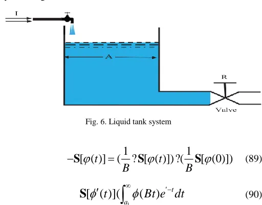
A tank with a heating system is displayed in Figure 1, where
5
.
0
~
R
, the thermal capacitance isC
~
2
also the temperature is
. The model is formulated as follows[10, 37],
)]
1
,
9
.
0
,
8
.
0
(
)),
,
0
(
),
,
0
(
[(
)
0
(
0
),
(
)
(
~1~p
r
r
T
t
t
t
RC
(71)By utilizing the FST method based on Z-number we obtain
)]
(
[
)]
(
[
t
S
t
S
(72)𝑆[𝜙′(𝐵𝑡)]⨀𝑒−𝑡𝑑𝑡 (73)
1 1 1 [ ( )]t ?( [ ( )]? (0))t [ ( )]?t (0)
B B B
S S S (74)
Therefore
1
1
[ ( )]
t
[ ( )]?
t
(0)
B
B
S
S
(75)Based on the Eq. (59), we have
)
,
0
(
)]
,
(
[
)]
,
(
[
)
,
0
(
)]
,
(
[
)]
,
(
[
1 1 1 1r
r
t
r
t
r
r
t
r
t
B B B B
S
S
S
S
(76)Therefore, the Z-number solution of Eq. (76) is extracted as
)]
1
,
94
.
0
,
8
.
0
(
)]),
,
(
[
)],
,
(
[
[(
S
t
r
S
t
r
p
whereFig. 1. A tank with a heating system
)
,
0
(
)
(
)
,
(
)
(
)]
,
(
[
)
,
0
(
)
(
)
,
0
(
)
(
)]
,
(
[
1 1 1 1 1 1 2 2 2 2r
r
t
r
t
r
r
r
t
B B B B B B
S
S
(77)By utilizing the inverse Sumudu transform for Z-numbers, we have
)
(
)
,
0
(
)
(
)
,
0
(
)]
,
(
[
)
(
)
,
0
(
)
(
)
,
0
(
)]
,
(
[
1 1 1 1 1 1 1 1 1 1 2 2 2 2 B B B B B Br
r
r
t
r
r
r
t
S
S
S
S
S
S
(78) where
)
(
)
(
)
,
(
)
(
)
(
)
,
(
2 ) , 0 ( ) , 0 ( 2 ) , 0 ( ) , 0 ( 2 ) , 0 ( ) , 0 ( 2 ) , 0 ( ) , 0 ( r r t r r t r r t r r te
e
r
t
e
e
r
t
(79)By considering case 2 for Z-numbers the following relation is obtained
1
1
[ ( )]
t
(
[ ( )]) ?(
t
(0))
B
B
S
S
(80)Hence
1
1
[ ( )]
t
(
[ ( )]) ?(
t
(0))
B
B
S
S
(81)Based on the above relations, Eq. (71) is illustrated as
)
,
0
(
)]
,
(
[
)]
,
(
[
)
,
0
(
)]
,
(
[
)]
,
(
[
1 1 1 1r
r
t
r
t
r
r
t
r
t
B B B B
S
S
S
S
(82)So, the Z-number solution of Eq. (82) is displayed as
)]
1
,
9
.
0
,
8
.
0
(
)]),
,
(
[
)],
,
(
[
[(
S
t
r
S
t
r
p
where
)
)(
,
(
)]
,
(
[
)
)(
,
0
(
)]
,
(
[
1 1 1 1 B Br
t
r
t
r
r
t
S
S
(83)By utilizing the inverse Sumudu transform for Z-numbers, we have
)
(
)
,
0
(
)
,
(
)
(
)
,
0
(
)
,
(
1 1 1 1 1 1 B Br
r
t
r
r
t
S
S
(84) where
)
,
0
(
)
,
(
)
,
0
(
)
,
(
r
e
r
t
r
e
r
t
t t
(85)If the initial condition is taken to be a symmetric triangular Z-number as
(
0
)
[(
a
(
1
r
),
a
(
1
r
)),
p
(
0
.
8
,
0
.
9
,
1
)],
soCase 1 :
))
1
(
(
)
,
(
))
1
(
(
)
,
(
r
a
e
r
t
r
a
e
r
t
t t
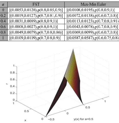
(86) Case 2:Table 1. Approximation errors based on Z-numbers
))
1
(
(
)
,
(
))
1
(
(
)
,
(
r
a
e
r
t
r
a
e
r
t
t t
(87)Approximation errors based on Z-numbers are shown in Table 1. These errors are the differences between the exact and the approximation solutions, for two different methods: FST and Average Euler method [38].
The following formula is utilized to transfer the Z-numbers to fuzzy numbers,
d
d
P P)
(
)
(
By taking in to considerationZ(B,~p)[(0.0078,0.0195),
)] 94 . 0 , 86 . 0 , 8 . 0 (
p , we obtain