INTERACTIVE LEARNING MODULES FOR PID CONTROL Jos´e Luis Guzm´an∗,Karl J.Astr¨om˚ ∗∗,Sebasti´an Dormido ∗∗∗,
Tore H¨agglund∗∗,Yves Piguet∗∗∗∗
∗Dep. de Lenguajes y Computaci´on, Universidad de Almer´ıa, 04120 Almer´ıa, Spain. E-mail:[email protected]
∗∗Department of Automatic Control, Lund University, Box 118 SE-22100 Lund, Sweden. E-mail: [email protected] ∗∗∗Dep. Inform´atica y Autom´atica, ETSI Inform´atica, UNED, 28040
Madrid, Spain. E-mail: [email protected]
∗∗∗∗Calerga S`arl, 35, av. de la Chabli`ere, 1004 Lausanne, Switzerland. E-mail: [email protected]
ABSTRACT
This paper describes a collection of interactive learn-ing modules for PID control based on the graphical spread sheet metaphor. The modules are designed to speed-up learning and to enhance understanding of the behavior of loops with PID controllers. The modules are implemented in Sysquake, a Matlab dialect with strong support of interaction. Executable versions of the modules for Mac and PC are available on the web.
1. INTRODUCTION
The idea to change properties and immediately being able to see the effects of the changes is very powerful both for learning and for designing. The dynamics of the changes provides additional information that is not available in static plots. An early effort to use interaction was made in the late 1970s by Bricklin and Frankston [3]. They developed VisiCalc which was based on the spread sheet metaphor. It contained a grid of rows and columns offigures forfinancial calcula-tions. Its implementation on the Apple II was one of the reasons why personal computers started to be used in the office. VisiCalc changed spread sheet from a calculation tool to a modeling and optimization tool. The implementation called Excel is now a standard tool in all offices.
Spread sheets were easy to implement because they only dealt with numbers. In control we have much richer graphical objects, but the value of having in-terconnected graphs that can be manipulated directly
has a great potential to enhance learning. The program VisiDyn [5] was an early implementation. Another attempt was made by Blomdell [2], who implemented a system on the Macintosh. This system has several novel features. A frame was used in the pole-zero dia-grams to indicate poles and zeros outside the plotting range. A novel way of dragging Bode plots was also introduced.
The early programs were useful but their implemen-tation required a substantial effort which significantly limited their use in education. Advances in computers and software has made implementation easier. Mat-lab has been used in several projects. Two successful efforts have resulted in ICTools [7] and CCSdemo [10]. The programs are, however, strongly version-dependent which has made support and future devel-opment cumbersome. Yves Piguet at the Federal In-stitute of Technology in Lausanne (EPFL) developed a Matlab-like program Sysquake which has strong support for interactive graphics [8], [9]. Projects based on Sysquake were developed at EPFL and elsewhere, see [8], [4], [6]. Early versions of tools for PID were developed by Piguet andAstr¨om in 2000.˚
The interactive tools can be very helpful in education but there is a danger that students try to obtain a good controller by manipulation without understand-ing. The tools should challenge the students and en-couraging them to make observations and relate them to theory in order to develop a broader and deeper understanding.
There are many interesting issues that have to be dealt with when developing interactive tools for control
which are related to the particular graphics represen-tations used. It is straight forward to see the effects of parameters on the graphics but not so obvious how the graphical objects should be manipulated. There are natural ways to modify pole-zero plots for example by adding poles and zeros and by dragging them. Bode plots can be manipulated by dragging the intersections of the asymptotes. However, it is less obvious how a Nyquist plot should be changed.
In the process of writing the book [1] the idea emerged that it would be useful to try to develop interactive learning modules (ILMs) for PID control. The idea was to develop interactive learning tools which could be used for introductory control courses at universi-ties and other schools, and for engineers in industry. The modules should be self-contained, they should be suitable both for self-study, for courses, and for demonstrations in lectures, and they should not require any additional software. Several attempts were made to structure the material. We started with the idea of a single module, but for practical reasons we ended up with several interactive learning modules. In this paper we describe three modules; PID Basics, PID Loop Shaping, andPID Windup. Work is in progress for additional modules. The modules are implemented in Sysquake. The main reasons for choosing Sysquake was its power to develop interactive graphical tools and the possibility to generate executable files that can run independently and distributed without any li-cences.
Notice that the interactive learning modules have been recently developed and feedback from the students is not yet available. The modules will be used in dif-ferent control courses at Lund University, University of Almer´ıa, UNED, and EPFL. One consideration that must be kept in mind is that the tool’s main feature, in-teractivity, cannot be easily illustrated in a written text. Nevertheless, some of the advantages of the applica-tions are shown in the paper. The reader is cordially invited to visit the web site (atwww.calerga.com) to experience the interactive features of the modules.
2. PID ESSENTIALS
In spite of all the advances in control theory the PID controller is still the workhorse of control which can be used to solve a large variety of control problems. The controller is used by persons with a wide range of control knowledge. In most cases derivative action is not used so the controller is actually a PI controller. Under certain conditions derivative action can, how-ever, give substantial improvement.
There are many different forms of PID controllers. Linear behavior differs in how set points are handled and how signals arefiltered. The derivative term is of-tenfiltered by afirst-orderfilter but an ideal derivative can also be combined with second-orderfiltering of the measured signal. All practical PID controllers are provided with some facility for avoiding windup of the
integrator if the actuator saturates. All these factors are discussed in depth in [1].
Because of its wide spread use, many aspects of PID control have been developed outside the main stream of control theory, which has had some unfortunate consequences. There is for example a long continuing debate if controllers should be tuned for load dis-turbance response or for set-point response, an issue which is completely bypassed by using a structure having two degrees of freedom. Set-point weighting is a simple way to obtain the advantages of a structure with two degrees of freedom.
In control literature it is customary to show only responses to steps in load disturbances or set-points. At best the control signals required to achieve the responses are also shown. The development of H∞
theory has shown that it is necessary to show at least six responses to completely characterize the behavior of a closed loop system. In [1] these responses are referred to as The Gang of Six. When developing the interactive tool we have made sure that all six responses are shown. Performance and robustness are also quantified in many different ways.
3. THE MODULES
The interactive learning modules have been developed to make it possible to quickly obtain a good intu-ition and a good working knowledge of PID control. The modules consist of menus where process transfer functions and PID controllers can be chosen, param-eters can be set, and results stored and loaded. A graphic display which shows time or frequency re-sponses is a central part. The graphics can be manipu-lated directly by dragging points, lines, and curves or by using sliders. Parameters that characterize robust-ness and performance are also displayed.
This paper describes three modules. The central mod-ule is calledPID Basics, two auxiliary modulesPID Loop ShapingandPID Windupillustrate loop shaping and windup. More modules are under development.
3.1 PID Basics
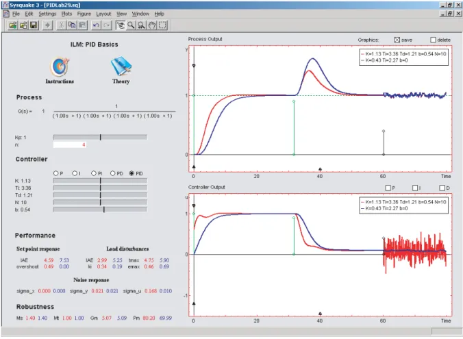
A simple and intuitive way to understand PID control is to look at the responses of the closed-loop system in the time domain and to observe how the responses depend on the controller parameters. To have a rea-sonably complete understanding of a feedback loop it is essential to consider six responses,the Gang of Six, see [1]. One possibility is to show process output and controller output for step commands in set-point and load disturbances and the response to noise in the sensor. The screen is set up for this configuration when you start it, see Figure 1. The picture on the screen is a dynamic version of Figure 4.2 in [1]. The module has a fast simulator of a closed-loop system and with a graphical user interface. It is also possible to see
Fig. 1. The user interface of the modulePID Basics. The plots show the time response of the Gang of Six. the frequency responses instead of the time responses.
Curves can be saved for easy comparison, and results can be loaded and stored for reporting.
The interaction is straight forward because it is done mainly by using sliders for controller parameters. Pro-cess models can be chosen from a menu which con-tains a wide range of transfer functions. It is also possible to enter an arbitrary transfer function in the Matlab rational function format. Process gain and time delay can be changed interactively. The PID controller has the structure
U(s) =K bYsp−Y+sT1 i E− sTd 1+sTd/N Y ,
whereU,Ysp,Y andE are the Laplace transforms of
control signal u, setpoint ysp, process output y, and
control errore=ysp−y, respectively. Controllers of
the types P, I, PD, PI and PID can be chosen and their parameters can be changed via menus or sliders. Values that characterize performance and robustness are also presented interactively.
A typical application is illustrated in Figure 1 which compares response of PI (K=0.432,Ti=2.43,b=
0) and PID (K =1.13, Ti =3.36, Td =1.21, b=
0.54,N=10) controllers for a process with the trans-fer function P(s) =1/(s+1)4. The PID controller
gives a better response to load disturbances by reacting faster, but the noise also generates more control action.
3.2 PID Loop Shaping
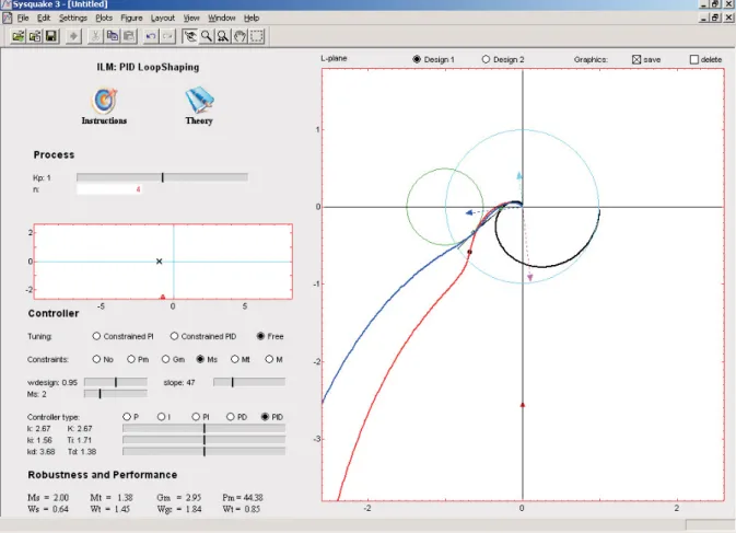
Loop shaping is a design method where it is attempted to choose a controller such that the loop transfer function obtains the desired shape. In this module the loop transfer function is illustrated by its Nyquist plot. The module shows the Nyquist plots of the process transfer functionP(s)and the loop transfer functions L(s) =P(s)C(s), see Figure 2. The key idea is that the action of the controller can be interpreted as mapping the process Nyquist plot to the Nyquist plot of the loop transfer function. For PI and PD control the mapping can be uniquely represented by mapping only one point. This point on the Nyquist plot of the process, which is called thedesign point, is characterized by its frequency. The corresponding point on the loop transfer function is called the target point. For PID control it is also possible to have an arbitrary slope of the loop transfer function at the target point. The module makes it possible to see the effects of the controller parameters and the effects of moving the design and target points.
Controllers can be represented in many different ways. In this module we use the parameterisation
C(s) =k+ksi+kds.
The loop transfer function is thus
L(s) =kP(s) +ksi+kds
P(s).
Fig. 2. The user interface of the modulePID Loop Shaping, showing bothFreeandConstrainedPID tuning. The point on the Nyquist curve of the loop transfer
function corresponding to the frequency ω is thus given by
L(iω) =kP(iω) +i−kωi+kdω
P(iω). (1) The proportional gain thus changesL(iω)in the di-rection of P(iω), integral gain ki changes it in the
direction of−iP(iω) and derivative gainkd changes
it in the direction ofiP(iω).
The design point is marked by a circle on the process transfer function which can be dragged. Alternative the frequency can be change by the slider marked (wdesign). The controller gainsk,ki, andkd can be
changed by dragging arrows as illustrated in Figure 2. The target point can be constrained to move on the unit circle, the sensitivity circles or to the real axis. In this way it is easy to make loop shaping with specifications on gain and phase margins or on the sensitivities. To find controller gains that gives the desired target point we divide (1) with P(iω) and take real and imaginary parts which gives
k=ReL(iω) P(iω)
−ωki+kdω=ImPL((iiωω))=A(ω).
(2)
Equation (2) gives directly the parameters of PI or PD controllers. An additional condition is required for a PID controller. To obtain this we observe that
L(s) =C(s)P(s) +C(s)P(s) =C(s)P(s) +L(Ps)(Ps)(s) =−sk2i+kd
P(s) +L(Ps)(Ps)(s).
The slope of the Nyquist curve is then given by dL(iω)
dω =iL(iω) =i ki
ω2+kd
P(iω)+iC(iω)P(iω).
This complex number has the argumentαif ImiL(iω)e−iα=0,
which implies that
ki ω2+kd= ReL(iω)PP(iω) (iω)e−iα ReP(iω)e−iα =B(ω). (3)
Combining this with (2) gives the controller parame-ters
ki=−ωA(ω) +ω2B(ω)
kd=A(ωω)+B(ω),
(4)
whereA(ω)andB(ω)are given by (2) and (3). Equa-tion (4) can be easily expressed in Sysquake using complex arithmetic, polynomial evaluation and poly-nomial ratio derivatives, or numerical derivatives if P(s)is not a rational transfer function with time delay. Figure 2 illustrates design a PID controller for a given sensitivity. The target point is moved to the sensitivity circle and the slope is adjusted so that the Nyquist curve is outside the sensitivity circle. The design and
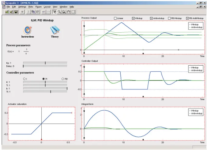
Fig. 3. The user interface of the modulePID Windup. The dashed vertical line makes it easy to compare times in the different graphs. In this particular case it is used to indicate when the process output enters the proportional band.
target points can be adjusted to maximize integral gain while maintaining a constraint on the complementary sensitivity. In the particular case we haveMs=Mt=2
and the controller parameters arek=2.51,ki=1.88
andkd=3.21.
3.3 PID Windup
Many aspects of PID control can be understood using linear models. There are, however, some important nonlinear effects that are very common even in simple loops with PID control. Integral windup can occur in loops where the process has saturations and the con-troller has integral action. When the process saturates the feedback loop is broken. If there is a control error the integral may reach large values and the control signal may be saturated for a long time resulting in large overshoots and undesirable transients.
The purpose of this module is to give a familiarity with the phenomenon of integral windup and a method for avoiding it, see [1]. The module shows process outputs and control signals for unlimited control signals, lim-ited control signals without anti-windup, and limlim-ited control signals with anti-windup, see Figure 3. Process models and controller parameters can be selected in the same way as in the other modules. The saturation limits of the control signal can be determined either
by entering the values or by dragging the lines in the saturation metaphor.
There are many different ways to protect against windup. Tracking is a simple method which is illus-trated in the block diagram in Figure 4. The system has an extra feedback path around the integrator. The signales is the difference between the nominal
con-troller outputvand the saturated controller outputu. If the saturated output is not directly available it can be obtained using a mathematical model of the satura-tion. The signales is fed to the input of the integrator
through gain 1/Tt. The signal es is zero when there
is no saturation. Under these circumstances it will not have any effect on the integrator. When the actuator saturates, the signal es is different from zero and it
will try to drive the integrator output to a value that such that the signalvis close to the saturation limit.
Actuator model Actuator − + Σ Σ Σ −y e=ysp−y K/Ti KTds 1/s 1/Tt es K v u
The notion of proportional band is useful to under-stand the windup effect. The proportional band is de-fined as the range of process outputs where the con-troller output is in the linear range. For a PI concon-troller, the proportional band is limited by
ymin=bysp+I−Kumax
ymax=bysp+I−Kumin.
The same expressions hold for PID control if we de-fine the proportional band as the band where the pre-dicted output yp=y+Tddy/dt is in the proportional
band(ymin,ymax). The proportional band has the width (umax−umin)/Kand is centred atbysp+I/K−(umax+
umin)/(2K). The proportional band can be shown in
the module.
Figure 3 illustrates windup and windup protection for a process with the transfer function P(s) =1/s where the controller saturates when the control signal has magnitude 0.2. The controller gains are k=1, Ti=1,b=1 and the tracking time constant isTt=1.
The curves shown represent system with and without windup protection. The proportional band for the con-troller with windup protection is also shown.
4. IMPLEMENTATION
The implementation of the modules is reasonably straight forward. Manipulation of graphical objects are well supported in Sysquake. Numerics for simu-lation consist of solving linear differential equations with constant coefficients and simple nonlinearities representing the saturations. For linear systems the complete system is sampled at constant sampling rate and the sampled equations are iterated. For systems with saturation the process and the controller are sam-pled separately withfirst order holds, the nonlineari-ties are added, and the difference equations are then iterated. It is straight forward to deal with delays be-cause the sampled systems are difference equations of finite order.
The numerical calculations for loop shaping are sim-ply manipulation of complex numbers. In this case we can deal with more general classes of systems by using symbolic representations of functions. The transfer functionP(s) =1/cosh√scan be represented as P=’1/cosh(sqrt(s))’. In the plots we have to evaluate the loop transfer function for complex argu-ments which is done in the following way
w=logspace(-2,2,500); s=i*w;
P=’1/cosh(sqrt(s))’; Pv=eval(P);
In this way we can represent systems that are de-scribed by partial differential equations.
The strong reasons for choosing Sysquake are its power to develop interactive graphical tools and the
facility to generate executablefiles that can run inde-pendently and distributed without any licence restric-tions.
5. SUMMARY
Three interactive learning modules for PID control, PID Basics,PID Loop ShapingandPID Windup, have been described. The modules are an attempt to make figures in the book [1] interactive. The purpose is to enhance learning by exploiting the advantages of immediately seeing the effects of changes that can never be shown in static pictures, e.g. like thefigures in [1]. The modules are implemented in Sysquake, a Matlab-like language with fast execution and excel-lent facilities for interactive graphics. The modules are available on the web atwww.calerga.com. Addi-tional modules for modeling, model reduction, design, Smith predictor, coupled loops and feedforward are under development.
REFERENCES
[1] Karl Johan Astr¨om and Tore H¨agglund.˚ Ad-vanced PID Control. ISA - The Instrumentation, Systems, and Automation Society, Research Tri-angle Park, NC 27709, 2005.
[2] Anders Blomdell. Spread-sheet for dynamic sys-tems — A graphic teaching tool for automatic control. Wheels for the Mind Europe, 2:46–47, 1989.
[3] D Bricklin and B Frankston. Visicalc ’79. Cre-ative Computing, 84.
[4] S. Dormido. The role of interactivity in control learning. 6th IFAC Symposium on Advances in
Control Education, pages 11–22, 2003. Oulu, Finland.
[5] E. Granbom and Tomas Olsson. VISIDYN—An interactive program for design of linear dynamic systems. Technical Report TFRT-5375, Depart-ment of Automatic Control, Lund Institute of Technology, Sweden, November 1987.
[6] J. L. Guzm´an, M. Berenguel, and S. Dormido. In-teractive teaching of constrained generalized pre-dictive control.IEEE Control Systems Magazine, 25(2):52–66, 2005.
[7] M. Johansson, M. G¨afvert, and K.J.Astr¨om. In-˚ teractive tools for education in automatic control. IEEE Control Systems Magazine, 18(3):33–40, 1998.
[8] Y. Piguet, U. Holmberg, and R. Longchamp. In-stantaneous performance visualization for graph-ical control design methods. 14th IFAC World Congress, 1999. Beijing (China).
[9] Y. Piguet.Sysquake 3 User Manual.Calerga S`arl, Lausanne, Switzerland, 2004.
[10] B. Wittenmark, H. Haglund, and M. Johansson. Dynamic pictures and interactive learning.IEEE Control Systems Magazine, 18(3):26–32, 1998.