ASSOCIATION RULE MINING BASED VIDEO CLASSIFIER WITH LATE ACCEPTANCE HILL CLIMBING APPROACH

MINIATURIZATION OF INERTIAL MAGNETOELECTRIC

VIBRATION VELOCITY SENSOR WITH HIGH FREQUENCY

RESPONSE AT LOW FREQUENCY BAND

1 _{XI CHEN,} 2 _{SHUIBAO YU}

1

College of Mathematics, Physics and Information Engineering, Zhejiang Normal University, Jinhua,

321004, Zhejiang, China.

2_{College of Mathematics, Physics and Information Engineering, Zhejiang Normal University, Jinhua,}

321004, Zhejiang, China.

E-mail: [email protected] , [email protected]

ABSTRACT

The frequency response of the inertial magnetoelectric vibration velocity sensor is limited in the low frequency range due to the character of second order high pass filter of the structure. For better performance in the low frequency range, the traditional method is to increase the initial mass of the sensor which will increase the size and weight tremendously. This paper presents a frequency-selected compensation network to improve the performance of the frequency response at low frequency band, keeping the sensor in small size and light weight. The frequency-selected network, which is composed of amplifiers, resisters and capacitances, is connected to the output port of the sensor in cascade without any modification of the sensor’s structure. After compensation, the frequency band of the sensor is flattened and the frequency response still has the character of second order high pass filter while the resonant frequency decreases from 10Hz to about 0.9Hz. The experimental results have shown that the sensor after been compensated has good performance in the low frequency range.

Keywords: Magnetoelectric Vibration Velocity Sensor, Compensation Network, Transfer Function,

Resonant Frequency, Low Frequency Band

1. INTRODUCTION

Some vibrations, such as seismic wave, bridge vibration, vibration of water turbine, have no static reference point relative to inertial space. Low frequency components in these vibrations are always ignored since the small acceleration values could hardly be experienced. But in some area, such as industrial machines, it is significant to monitor low frequency vibrations which are vital indicators of their health [1]. Low frequency vibration detection in these fields is mainly based on high sensitivity, excellent performance, good reliability inertial sensor which has frequency range from 1Hz to 1 kHz at least [2–4]. Several kinds of sensors have been proposed in relevant researches to detect the absolute vibration (The vibration which has no static reference point relative to inertial space), such as fiber optic sensor based on Fiber Bragg Grating (FBG) [5–8], piezoelectric vibration sensor [9–11], magnetoelectric velocity sensor or accelerometer [12, 13]. In every particular

application, there has the most appropriate sensor for it [14].

One of the most widely used sensors in the low frequency absolute vibration detection is the inertial magnetoelectric velocity sensor which has the advantages of wide bandwidth (10-1000Hz), low output impedance, high resolution and low cost [15–16]. All inertial sensors using an electrical field share a basic structure called spring-mass system [17, 18]. The inertial magnetoelectric velocity sensor with this structure has the character of second order band pass filter. In this case, the measurement of low frequency is limited due to the high frequency resonance.

dynamic characteristics of the structure to which it is mounted [20]. The typical practice to eliminate the mass loading effect is to use the lightest, smallest sensor that still satisfies all the performance requirements [14]. So it is significant to use efficient method for frequency response improvement at the condition of keeping the light and small spring-mass system.

In this paper, we investigated the amplitude-frequency characteristic of the inertial magnetoelectric velocity sensor. According to its model and transfer function, an optimized frequency-selected compensation network was put forward which expand the working bandwidth in the low frequency range. After compensation, it still has the advantages of fast real-time response, light and small spring-mass system.

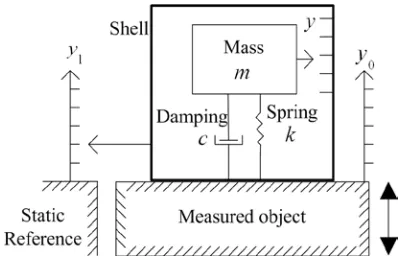
2. SENSOR MODEL

An inertial magnetoelectric velocity sensor is a mass supported on a spring and driven by an external force. The force in small sensor is normally generated electromagnetically. The suspended mass can either be the magnets with a supporting structure or in some cases the coil itself. A mechanical model of the inertial magnetoelectric velocity sensor is shown in Fig. 1.

Fig. 1. Mechanical Model Of An Inertial Magnetoelectric Velocity Sensor

It can be modeled by a simple spring-mass-damping assembly where mis the inertial mass,

k_{is spring constant and} c_{is the damping.}

Supposing y1 _{is absolute coordinate of the}

inertial mass, y0 _{is convected coordinate}

andyrepresents the relative coordinate, the motion equation can be described as

0

1 dy

dy dy

dt = dt +dt (1)

According to Newton’s second law, the kinetic equation can be established as

2 1 2

dy dy

m c ky

dt

d t = − − (2)

And the electromagnetic induction equation can be expressed as

( ) ( )

( ) dy t dy t

E t BNL

dt α dt

= = (3)

where Bis the magnetic induction intensity, N is the number of coil turns, Lis the average length of single-turn coil, α =BNL is the sensitivity. Assuming the exciter is making periodic sinusoidal vibration

0 sin

y = A ωt (4)

Then the solution of equation (2) can be given by

0 0

1 sin( ) sin( )

t

y=A e−ξ ω ω′t+ϕ′ +A′ ω ϕt− (5) where

2 2 2 2

0

/ (1 ) (2 )

A′=Aω′′ −ω′′ + ξ ω′′ (6)

2 0

tanϕ=2ξ ω′′/ (1−ω′′ ) (7)

Here, A1、ω'、ϕ'_{is constant,} ω′′ =ω ω/ 0_, f0 _is

resonant frequency,

0 2 f0 k m/

ω = π = (8)

is angular frequency of the sensor,

0 c/ 2 mk

ξ = (9)

is damping ratio. The first term in equation (5) will decrease rapidly with the increase of time. Therefore, it could be approximately written as follows

sin( )

y=A′ ω ϕt− (10)

It can be concluded from equation (10) that the inertial mass is making sinusoidal vibration and the vibration frequency is the same with the measured

object. When ω′′ >>1 and ξ <0 1 ， _{i.e., the}

vibration frequency of the measured object is much larger than the resonant frequency of the spring-mass-damping system, it can be obtained that

A′ =A，tanϕ=0. Hence, we have

sin( ) sin( ) sin( )

y=A′ ω ϕt− =A ω πt− = −A ωt (11)

0 ₀

dy dy

dt +dt = (12)

It means that the mass is in static state in absolute coordinate while the shell is making the same movement with the measured object.

decreasing the value of spring constant k , or increasing the inertial mass mcould reduce the resonant frequency. In gravity field, the

displacement y′of the spring can be expressed as

2 2

0 0

( ) (2 )

mg g g

y

k ω π f

′ = = = (13)

where g is constant of gravity acceleration.

Supposing the resonant frequency f0 =1 _{Hz, it}

could be calculated from equation (13) that the spring static elongation is more than 25cm long. Obviously, the size of the sensor is increased out of the requirement and the stability could hardly be satisfied.

3. COMPENSATION

3.1 Principle of Compensation

Appling Laplace transform to equations (1) – (3), the transfer function of the sensor can be deduced as

( )

0 0 0

2

s H s

s s

α

ξ ω ω

− =

+ + (14)

where s= jω , ω=2π f . Using equation (14), the magnitude and phase response of the sensor as a function of frequency and damping ratio can be calculated as shown in equation (15) and (16) respectively,

( )

(

)

0 0 0

( )

1 2

H jω αλ

λ ξ λ

=

 ₋  ₊

 

(15)

1 0 0

2 0

2

tan [ ]

1 ξ λ ϕ λ − = −

− (16)

whereλ =0 f / f0_{. Equation (14) shows that the}

transfer function has the character of second order high pass filter.

As shown in Fig. 2, it is feasible to seek a compensation network connected to the sensor in cascade when the compensated sensor system still has the character of second order high pass filter and the resonant frequency of the compensated sensor system is much lower than the uncompensated ones. The transfer function of the compensated sensor system can be expressed as

( )

0 0 0

2

2 2

1 1 1

( ) ( ) ( ) 2 2 o i V s

G s H s C s C s

V s s

s

s s

α

ξ ω ω

α

ξ ω ω

− = = ⋅ = ⋅ + + − = + + (17)

where ω1_{is equivalent angular frequency of the}

sensor system after been compensated, ξ1 _is

equivalent damping ratio.

Fig. 2. Schematic Of Amplitude-Frequency Characteristic Compensation

The magnitude and phase response of the compensated sensor system as can be calculated as

( )

(

)

2 1 2

2 2

1 1 1

( )

1 2

G jω αλ

λ ξ λ

=

 ₋  ₊

 

(18)

1 1 1

2 1

2

tan [ ]

1 ξ λ φ λ − = − − (19)

where λ =1 f / f1 _, f1 _{is equivalent resonant}

frequency. The transfer function of the compensation network, from equation (17), can be written as

2 2

0 0 0

2 2

1 1 1

2

( ) ( ) ( ) ( )

2 HP BP LP

s s

C s C s C s C s

s s

ξ ω ω

ξ ω ω

+ +

= = + +

+ + (20)

where

2

2 2

1 1 1

( )

2 HP

s

C s

s ξ ωs ω

=

+ + (21)

0 0

2 2

1 1 1

2 ( ) 2 BP s C s s s ξ ω

ξ ω ω

=

+ + (22)

2 0

2 2

1 1 1

( ) 2 LP C s s s ω

ξ ω ω

=

+ + (23)

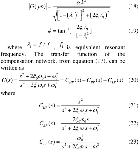
Fig. 3. Principle Block Diagram Of Frequency-Selected Compensation

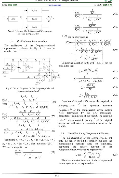
3.2 Realization of Compensation

The realization of the frequency-selected compensation is shown in Fig. 4. It can be concluded that

Fig. 4. Circuit Diagram Of The Frequency-Selected Compensation Network

2

5 6 4

5 3 4

2

2 5 6 4 6

1

5 3 4 1 1 5 1 2 1 2

( )

1 ( )

R R R

s

R R R

V s

R R R s R

V s s

R R R R C R R R C C

+ ⋅ + = + + ⋅ ⋅ + ⋅ + (24)

5 6 4

3 5 3 4 1 1

2 5 6 4 6

1

5 3 4 1 1 5 1 2 1 2

( )

1 ( )

R R R s

V s R R R R C

R R R s R

V s s

R R R R C R R R C C

+ _{⋅ ⋅} + = + + ⋅ ⋅ + ⋅ + (25)

5 6 4

5 3 4 1 2 1 2

4

2 5 6 4 6

1

5 3 4 1 1 5 1 2 1 2

1 ( )

1 ( )

R R R

R R R R R C C V s

R R R s R

V s s

R R R R C R R R C C

+ ⋅ ⋅ + = + + ⋅ ⋅ + ⋅ + (26)

SupposingC₁=C₂ =C ,R₅ =R₆=R₃ =R₄ =R ,

10 8

R =R , R₂ =2R₁=2R , then equations (24) – (26) can be simplified as

2 2 2 1 2 2 ( ) 1 ( ) 2

V s s

s V s

s

RC R C

= + + (27) 3 2 1 2 2 ( ) 1 ( ) 2 s

V s _RC

s V s

s

RC R C

= + + (28) 2 2 4 2 1 2 2 1

( ) ₂

1 ( )

2

V s _{R C}

s

V s _s

RC R C

=

+ +

(29)

( )

C s _{can be expressed as}

10 2 10 3 10 4

8 1 9 1 7 1

2 10 10

2 2 9 7 2 2 2 ( ) ( ) ( ) ( ) ( ) ( ) ( ) 1 2 1 2

R V s R V s R V s

C s

R V s R V s R V s

R s R

s

R RC R R C

s s

RC R C

  = −_ + + _    _{+ +}      = −  _{+ +}      (30)

Comparing equation (20) with (30), it can be concluded that 2 1 1 2 2 2 R R

ξ = = (31)

1

1 2 1 2

1 1

2 2 f

R R C C πRC

= = (32)

7 10 0 9 2 2 R R R

ξ = (33)

10 0 7 1 2 2 R f

R πRC

= (34)

Equation (31) and (32) mean the equivalent

damping ratio ξ1 _{and equivalent resonant}

frequency f1 _{of the compensated sensor system}

were determined by the R-C (resistance-capacitance) parameters of the circuit. The damping

ratio ξ0 _{and resonant frequency} f0 _{of the original}

sensor will influence the summation factor of the circuit.

3.3 Simplification of Compensation Network

For miniaturization of the sensor system, not only the sensor should be smaller, but also the compensation network need be simplified. Supposing the transfer function of the compensation network can be expressed as

2 2

0 0 0

2 2

1 1 1

2 ( ) 2 s s C s s s

ξ ω ω

ξ ω ω

+ +

′ =

− + (35)

( )

1 1 1

( ) ( )

2 s

G s H s C s

s s

α

ξ ω ω

−

′ = ⋅ ′ =

− + (36)

The magnitude and phase response of the compensated sensor system can be calculated as

( )

(

)

2 1 2

2 2

1 1 1

( )

1 2

G jω αλ

λ ξ λ

′ =

 ₋  ₊

 

(37)

1 1 1

2 1

2

tan [ ]

1 ξ λ φ

λ

−

′ =

− (38)

Comparing equation (18) with (37), (19) with (38), it could be concluded that the sensor system using these two kinds of compensation networks has the same magnitude response while the phase response is reverse.

Supposing f0 =10 _Hz, f1=1 _Hz, ξ =1 0.707 _,

0 0.707

ξ = _{, α =1，the simulation curves of the}

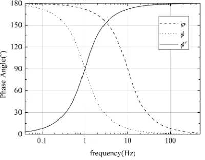
normalized frequency response before and after compensation can be plotted as shown in Fig. 5. The simulation curves of phase response before and after compensation are shown in Fig. 6. Obviously, the sensor has much better performance in frequency response at low frequency band after been compensated.

From Fig. 6, it can be seen that there is a corresponding time lag associated with a sensor’s output when compared to the input at frequencies near the natural frequency of the sensor. Data collected using the sensor is subject to considerable phase shifts when its frequency content is around the natural frequency of the sensor. The smaller phase errors, the more accurate data analysis will be.

The compensation network G s( ) translates the curve of the phase response to lower frequency direction, keeping the curve shape unchangeable. As a result, the compensated sensor has less phase error than the original one at the same frequency point. And both the phase response of the

compensation network G s'( ) and G s( ) have the same phase error. Therefore, according to equation (35), the circuit of compensation network could be simplified as shown in Fig. 7.

Fig. 5. Simulation Curves Of The Normalized Frequency Response Before And After Compensation

(f0=10Hz, f1=1Hz, ξ ξ1= 0=0.707，α =1)

Fig. 6. Simulation Curves Of Phase Response Before And After Compensation (f0=10Hz, f1=1Hz,

1 0 0.707

ξ ξ= = ，α =1)

Fig. 7. Simplified Circuit Diagram Of The Frequency-Selected Compensation Network

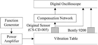
4. EXPERIMENT AND RESULTS

4.1 Experimental Setup

network was rigidly mounted on the vibration table (another commercially available inertial magnetoelectric velocity sensor, Bently 9200 from GE Measurement & Control Solutions, was also mounted on the vibration table for comparison test) which has the capability of controlling the vibration parameters precisely. The sensor was exposed to sinusoidal forces at different frequencies. The output signals from the sensors and compensation network were measured using a digital oscilloscope without any external signal conditioner or amplifier.

Fig. 8. Experimental system for vibration test

4.2 Parameters Determination

The nominal resonant frequency f0_{of the}

CS-CD-005 sensor and the damping ratio ξ0 _is

undetermined. The exact value of f0_andξ0_{can be}

obtained as follows: get a group of normalized

amplitudes A1_, A2_,A3_…… An_{with corresponding}

frequencies f1_, f2_, f3_…… fn _{, substituting them} into equation (15), we get

2

2 2

0 0

0

1

1 2

n

n n

A

f f

f ξ f

=

 _{ }  _{ }

 −_{ }  +_{ }

     

 

(39)

where nis natural number. Therefore, f0_, ξ0

can be derived as equation (40) and (41).

(

) (

)

0

2

2 2

0 0 2

1

1 2 1 2 1

n

n f

f

A

ξ ξ

=

 

− + − +_ − _

 

(40)

2 2 4 4

0 0 2

0

0

1

2 1

2 n n

n

n

f f f f

A

f f

ξ

 

− + _ − _

 

= (41)

Solving equation (40) and (41) yields n

solutions of f0 _and ξ0 _{. The average value of}

0

f _andξ0_{was used as final resonant frequency and}

damping ratio.

The test results at 200mm/s velocity is shown in table 1. The calculated average value of the

resonant frequency f0 _{was 10.409Hz and the}

damping ratio ξ0 _{was 0.523. Therefore, the main}

parameter values of the compensation network can be determined as shown in table 2. Fig. 9 is a photograph of the actual sensor that has been compensated by frequency-selected network.

Table I

Experimental Data Of Frequency Response For The Original Sensor Cs-Cd-005

Frequencyf_n (Hz) Normalized amplitudeA_n

5 0.276

10 0.869

15 1.141

20 1.103

30 1.003

Table II

Main Parameter Values Of The Compensation Network

Parameters Values Parameters Values

1

ξ 0.707 R(kΩ) 120

1

f (Hz) 0.9328 R₇(kΩ) 1.02

8

R (kΩ) 127 R₉(kΩ) 15.4

10

R (kΩ) 127 C(µF) 1

Fig. 9. Photograph Of The Sensor With Frequency-Selected Compensation Network

4.3 Experimental Setup

A clear comparison between the theoretical

experimental ones before and after compensation is shown in Fig. 10. It shows that the experimental normalized frequency response is very close to the theoretical ones. Some experimental data deviated from the theoretical curve is due to an approximation of theR, Cvalue. The normalized frequency response before compensation has small resonant peak and was flattened after been compensated.

Experimental comparison between 9200 and compensated CS-CD-005 were also carried out. The main parameters for comparison are listed in table 3. The sensor CS-CD-005 we used for compensation has much smaller size and weight than 9200, but higher resonant frequency. However, the resonant frequency of the CS-CD-005 sensor decreases from 10Hz to 0.93 Hz after been compensated while it still keeps the small size and light weight.

Table III

Main Parameters For Comparison Between 9200 And Compensated Cs-Cd-005

Parameters 9200 CS-CD-005

Compensated CS-CD-005 Height (mm) 102 33 43.1 Diameter (mm) 41 26 28.5 Weight(g) 480 78 90.2 Frequency

Response (Hz, -3dB)

5-1000 10-1000 0.93-1000

Sensitivity (mV/(mm·s-1_),

100Hz)

20 100 100

Dynamic Operating

Range (mm) 2.54 2.0 2.0

Fig. 10. Experimental And Theoretical Frequency Responses Before And After Compensation (f0=10.409Hz, f1=0.9328Hz, ξ0=0.523, ξ1=0.707)

Fig. 11. Output Waveform Quality Comparison Between 9200 And Compensated CS-CD-005 At

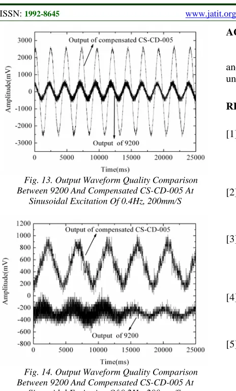
Sinusoidal Excitation Of 10 Hz, 400mm/S The comparison of the output waveform quality between 9200 and compensated CS-CD-005 at different frequencies with the same sinusoidal excitation velocity is shown in Figs. 11-14. Obviously, the compensated CS-CD-005 has better performance in frequency response in the low frequency range. It should be pointed out that the output waveform of 9200 has little distortion at 0.4Hz while the compensated ones of CS-CD-005 still has good waveform quality. Both 9200 and compensated CS-CD-005 output waveforms were distorted seriously at 0.2Hz. However, the output waveform of compensated CS-CD-005 can still reflect the characteristic of sinusoidal vibration while the ones of 9200 is submerged in noise.

Fig. 12. Output Waveform Quality Comparison Between 9200 And Compensated CS-CD-005 At

Fig. 13. Output Waveform Quality Comparison Between 9200 And Compensated CS-CD-005 At

Sinusoidal Excitation Of 0.4Hz, 200mm/S

Fig. 14. Output Waveform Quality Comparison Between 9200 And Compensated CS-CD-005 At

Sinusoidal Excitation Of 0.2Hz, 200mm/S.

5. CONCLUSION

The inertial magnetoelectric velocity sensor has the character of second order high pass filter and the resonant frequency cannot be very low according to the mechanical model. Since the frequency response cannot meet the demand in the low frequency range, the scope of application is limited. To improve the performance at low frequency, a frequency-selected network for amplitude-frequency characteristic compensation was developed. Experimental verification was performed and found to be in good agreement with the theoretical analysis.

At the circumstance of unchanging the original sensor’s structure, the frequency-selected network improved the frequency response in the low frequency range by changing theR, Cparameters of the circuit. Therefore, it still has the characters of small size and light weight. It can meet the demand in vibration measurement especially in the low frequency range.

ACKNOWLEDGEMENTS

This work was supported in part by the Science and Technology Hall of Zhejiang Province in China under Grant 2009C31006.

REFRENCES:

[1] T. K. Gangopadhyay, Prospects for Fibre Bragg Gratings and Fabry-Perot Interferometers in fibre-optic vibration sensing, Sensors and Actuators A, vol. 113, n. 1, pp. 20–38, 2004.

[2] T. C. Liang, Y. L. Lin, Ground vibrations detection with fiber optic sensor, Optics Communications, vol. 285, n. 9, pp. 2363– 2367, 2012.

[3] Y. Itakura, N. Fujii, T. Sawada, Basic characteristics of ground vibration sensors for the detection of debris flow, Physics and Chemistry of the Earth, Part B, vol. 25, n. 9, pp. 717–720, 2000.

[4] D. Pfeffer, C. Hatzfeld, R. Werthschützky, Development of an electrodynamic velocity sensor for active mounting structures, Procedia Engineering, vol. 25, pp. 547–550, 2011. [5] J. Wu, V. Masek, M. Cada, The possible use of

fiber Bragg grating based accelerometers for seismic measurements, Canadian Conference on Electrical and Computer Engineering (Page: 860–863 Year of Publication: 2009 ISBN: 978-1-4244-3508-1) .

[6] N. Basumallick, I. Chatterjee, P. Biswa, et al., Fiber Bragg grating accelerometer with enhanced sensitivity, Sensors and Actuators A, vol. 173, n. 1, pp. 108–115, 2012.

[7] L. H. Kang, D. K. Kim, J. H. Han, Estimation of dynamic structural displacements using fiber Bragg grating strain sensors, Journal of Sound and Vibration, vol. 305, n. 3, pp. 534–542, 2007.

[8] F.Xie, J. Ren, Z. Chen, et al., Vibration-displacement measurements with a highly stabilised optical fiber Michelson interferometer system, Optics & Laser Technology, vol. 42, n. 1, pp. 208–213, 2010. [9] T. Li, Y. H. Chen, J. Ma, Frequency

dependence of piezoelectric vibration velocity, Sensors and Actuators A, vol. 138, n. 2, pp. 404–410, 2007.

[11]S. Shanmugavel, K. Yao, T. D. Luong, et al., Miniaturized acceleration sensors with in-plane polarized piezoelectric thin films produced by micromachining, IEEE Transactions on Ultrasonics, Ferroelectrics and Frequency Control, vol. 58, no. 11, pp. 2289-2296, 2011. [12]S. Wakui, A. Noda, T. Akiyama, et al.,

Development of velocity sensor with high frequency band and its application to a vibration isolate table, Precision Engineering, vol.31, pp. 146–155, 2007.

[13]A. S. Ebrahim, R. S. Huang, C. Y. Kwok, A linear electromagnetic accelerometer, Sensors and Actuators A, vol. 44, no. 2, pp. 103-109, 1994.

[14]J. Shieh, J. E. Huber, N. A. Fleck, et al., The selection of sensors, Progress in Materials Science, vol. 46, no. 3-4, pp. 461-504, 2001. [15]X. Yi, P. Yan, H. Zhang, et al., Vibration

measurement of railway bridge with seismic low-frequency transducer based on signal reconstruction technique, Proceedings of SPIE-The International Society for Optical Engineering (Page: 201-208 Year of Publication: 1996 ISBN: 0471970247 ).

[16]L. Benassi, S. J. Elliott, Active vibration isolation using an inertial actuator with local displacement feedback control, Journal of Sound and Vibration, vol. 278, no. 4-5, pp. 705–724, 2004.

[17]I. Lee, G. H. Yoon, J. Park, et al., Development and analysis of the vertical capacitive accelerometer, Sensors and Actuators A, vol. 119, no. 1, pp. 8–18, 2005. [18]W. Hernández, Improving the response of an

accelerometer by using optimal filtering, Sensors and Actuators A, vol. 88, no. 3, pp. 198-208, 2001.

[19]F. Braghin, S. Cinquemani, F. Resta, A low frequency magnetostrictive inertial actuator for vibration control, Sensors and Actuators A, vol. 180, pp. 67–74, 2012