Turbo Coding, Turbo Equalisation and Space Time Coding

(1)

Turbo Coding, Turbo Equalisation and

Space-Time Coding

by

c

L. Hanzo, T.H. Liew, B.L. Yeap

(2)

Contents

Preface xiii

Acknowledgments xxv

I

Convolutional and Block Coding

1

1 Convolutional Channel Coding 3

1.1 Brief Channel Coding History . . . 3

1.2 Convolutional Encoding . . . 4

1.3 State and Trellis Transitions . . . 6

1.4 The Viterbi Algorithm . . . 7

1.4.1 Error-Free Hard-Decision Viterbi Decoding . . . 7

1.4.2 Erroneous Hard-Decision Viterbi Decoding . . . 11

1.4.3 Error-Free Soft-Decision Viterbi Decoding . . . 13

1.5 Summary and Conclusions . . . 15

2 Block-Based Channel Coding 17 2.1 Introduction . . . 17

2.2 Finite Fields . . . 18

2.2.1 Definitions . . . 18

2.2.2 Galois Field Construction . . . 21

2.2.3 Galois Field Arithmetic . . . 23

2.3 Reed-Solomon and Bose-Chaudhuri-Hocquenghem Block Codes . . . 24

2.3.1 Definitions . . . 24

2.3.2 RS Encoding . . . 26

2.3.3 RS Encoding Example . . . 28

2.3.4 Linear Shift-Register Circuits for Cyclic Encoders . . . 32

2.3.4.1 Polynomial Multiplication . . . 32

2.3.4.2 Systematic Cyclic Shift-Register Encoding Example . . . . 33

2.3.5 RS Decoding . . . 35

(3)

2.3.5.1 Formulation of the Key Equations [1–9] . . . 35

2.3.5.2 Peterson-Gorenstein-Zierler Decoder . . . 40

2.3.5.3 PGZ Decoding Example . . . 42

2.3.5.4 Berlekamp-Massey Algorithm [1–9] . . . 48

2.3.5.5 Berlekamp-Massey Decoding Example . . . 54

2.3.5.6 Computation of the Error Magnitudes by the Forney Algo-rithm . . . 57

2.3.5.7 Forney Algorithm Example . . . 61

2.3.5.8 Error Evaluator Polynomial Computation . . . 63

3 Soft-Decoding and Performance of BCH Codes 67 3.1 Introduction . . . 67

3.2 BCH codes . . . 67

3.2.1 BCH Encoder . . . 69

3.2.2 State and Trellis Diagrams . . . 71

3.3 Trellis Decoding . . . 73

3.3.1 Introduction . . . 73

3.3.2 Viterbi Algorithm . . . 73

3.3.3 Hard Decision Viterbi Decoding . . . 76

3.3.3.1 Correct Hard Decision Decoding . . . 76

3.3.3.2 Incorrect Hard Decision Decoding . . . 76

3.3.4 Soft Decision Viterbi Decoding . . . 77

3.3.5 Simulation Results . . . 79

3.3.5.1 The Berlekamp-Massey Algorithm . . . 79

3.3.5.2 Hard Decision Viterbi Decoding . . . 82

3.3.5.3 Soft Decision Viterbi Decoding . . . 82

3.3.6 Conclusion On Block Coding . . . 84

3.4 Soft Input Algebraic Decoding . . . 84

3.4.2 Chase Algorithms . . . 89

3.4.2.1 Chase Algorithm 1 . . . 92

3.4.2.2 Chase Algorithm 2 . . . 94

II

Turbo Convolutional and Turbo Block Coding

99

4 Turbo Convolutional Coding 101 4.1 Introduction . . . 101

4.2 Turbo Encoder . . . 102

4.3 Turbo Decoder . . . 104

4.3.2 Log Likelihood Ratios . . . 105

(4)

4.3.3.1 Introduction and Mathematical Preliminaries . . . 108

4.3.3.2 Forward Recursive Calculation of the k (s)Values . . . . 112

4.3.3.3 Backward Recursive Calculation of the k (s)Values . . . . 113

4.3.3.4 Calculation of the k (s;s)Values . . . 114

4.3.3.5 Summary of the MAP Algorithm . . . 117

4.3.4 Iterative Turbo Decoding Principles . . . 118

4.3.4.1 Turbo Decoding Mathematical Preliminaries . . . 118

4.3.4.2 Iterative Turbo Decoding . . . 120

4.3.5 Modifications of the MAP algorithm . . . 124

4.3.5.1 Introduction . . . 124

4.3.5.2 Mathematical Description of the Max-Log-MAP Algorithm 124 4.3.5.3 Correcting the Approximation – the Log-MAP Algorithm . 128 4.3.6 The Soft-Output Viterbi Algorithm . . . 128

4.3.6.1 Mathematical Description of the SOVA Algorithm . . . 128

4.3.6.2 Implementation of the SOVA Algorithm . . . 131

4.3.7 Turbo Decoding Example . . . 133

4.3.8 Comparison of the Component Decoder Algorithms . . . 141

4.3.9 Conclusions . . . 145

4.4 Turbo Coded BPSK Performance Over Gaussian Channels . . . 146

4.4.1 Effect of the Number of Iterations Used . . . 146

4.4.2 Effects of Puncturing . . . 148

4.4.3 Effect of the Component Decoder Used . . . 149

4.4.4 Effect of the Frame-Length of the Code . . . 150

4.4.5 The Component Codes . . . 152

4.4.6 Effect of the Interleaver . . . 155

4.4.7 Effect of Estimating the Channel Reliability ValueL c. . . 159

4.5 Turbo Coding Performance Over Rayleigh Channels . . . 164

4.5.2 Performance Over Perfectly Interleaved Narrow-Band Rayleigh Channels . . . 164

4.5.3 Performance Over Correlated Narrow-Band Rayleigh Channels . . . 166

5 The Super-Trellis Structure of Convolutional Turbo Codes 171 5.1 Introduction . . . 171

5.2 System model and terminology . . . 172

5.3 Introducing the turbo code super-trellis . . . 175

5.3.1 Turbo encoder super-state . . . 175

5.3.2 Turbo encoder super-trellis . . . 177

5.3.3 Generalised Definition of the Turbo Encoder Super–States . . . 178

5.3.4 Example of a super-trellis . . . 182

5.4 Complexity of the turbo code super-trellis . . . 186

5.4.1 Rectangular interleavers . . . 186

5.4.2 Uniform interleaver . . . 187

5.5 Optimum decoding of turbo codes . . . 189

(5)

5.5.2 Comparison with conventional convolutional codes . . . 194

5.6 Discussion of the results . . . 194

5.8 Appendix: Proof of algorithmic optimality . . . 199

6 Turbo BCH Coding 203 6.1 Introduction . . . 203

6.2 Turbo Encoder . . . 204

6.3 Turbo Decoder . . . 205

6.3.1 Log Likelihood Ratio . . . 206

6.3.2 Soft Channel Output . . . 208

6.3.3 The Maximum A-Posteriori Algorithm . . . 209

6.3.3.1 Calculation of the k (s;s)Values . . . 212

6.3.3.2 Forward Recursion . . . 213

6.3.3.3 Backward Recursion . . . 214

6.3.3.4 Summary of the MAP Algorithm . . . 215

6.3.4 Modifications of the MAP algorithm . . . 218

6.3.4.1 Introduction . . . 218

6.3.4.2 Max-Log-MAP Algorithm . . . 218

6.3.4.3 Log-MAP Algorithm . . . 220

6.3.5 The Soft Output Viterbi Algorithm . . . 220

6.3.5.1 SOVA Decoding Example . . . 223

6.4 Turbo Decoding Example . . . 226

6.5 MAP Algorithm For Extended BCH codes . . . 233

6.5.2 Modified MAP Algorithm . . . 235

6.5.2.1 The Forward and Backward Recursion . . . 235

6.5.2.2 Transition Probability . . . 236

6.5.2.3 A-Posteriori Information . . . 237

6.5.3 Max-Log-MAP and Log-MAP Algorithm for Extended BCH codes . 238 6.6 Simulation Results . . . 240

6.6.1 Number of Iterations Used . . . 241

6.6.2 The Decoding Algorithm . . . 242

6.6.3 The Effect of Estimating the Channel Reliability ValueL c . . . 244

6.6.4 The Effect of Puncturing . . . 245

6.6.5 The Effect of the Interleaver Length of the Turbo Code . . . 246

6.6.6 The Effect of the Interleaver Design . . . 248

6.6.7 The Component Codes . . . 250

6.6.8 BCH(31;k;d min) Family Members . . . 253

6.6.9 Mixed Component Codes . . . 254

6.6.10 Extended BCH codes . . . 255

6.6.11 BCH Product codes . . . 256

(6)

7 Redundant Residue Number System Codes 259

7.1 Introduction . . . 259

7.2 Background . . . 261

7.2.1 Conventional Number System . . . 261

7.2.2 Residue Number System . . . 262

7.2.3 Mixed Radix Number System . . . 263

7.2.4 Residue Arithmetic Operations . . . 264

7.2.4.1 Multiplicative Inverse . . . 265

7.2.5 Residue to Decimal Conversion . . . 266

7.2.5.1 Chinese Remainder Theorem . . . 266

7.2.5.2 Mixed Radix Conversion . . . 268

7.2.6 Redundant Residue Number System . . . 270

7.2.7 Base Extension . . . 271

7.3 Coding Theory of Redundant Residue Number Systems . . . 273

7.3.1 Minimum Free Distance of RRNS Based Codes . . . 273

7.3.2 Linearity of RRNS Codes . . . 276

7.3.3 Error Detection and Correction in RRNS Codes . . . 277

7.4 Multiple Error Correction Procedure . . . 279

7.5 RRNS Encoder . . . 286

7.5.1 Non-systematic RRNS Code . . . 286

7.5.2 Systematic RRNS Code . . . 289

7.5.2.1 Modified Systematic RRNS Code . . . 290

7.6 RRNS Decoder . . . 291

7.7 Soft Input and Soft Output RRNS Decoder . . . 292

7.7.1 Soft Input RRNS Decoder . . . 292

7.7.2 Soft Output RRNS Decoder . . . 294

7.7.3 Algorithm Implementation . . . 297

7.8 Complexity . . . 299

7.9 Simulation Results . . . 303

7.9.1 Hard Decision Decoding . . . 305

7.9.1.1 Encoder Types . . . 305

7.9.1.2 Comparison of Redundant Residue Number System codes and Reed-Solomon Codes . . . 306

7.9.1.3 Comparison Between Different Error Correction Capabili-tiest . . . 306

7.9.2 Soft Decision Decoding . . . 309

7.9.2.1 Effect of the Number of Test Positions . . . 309

7.9.2.2 Soft Decision RRNS(10,8) Decoder . . . 310

7.9.3 Turbo RRNS Decoding . . . 310

7.9.3.1 Algorithm Comparison . . . 310

7.9.3.2 Number of Iterations Used . . . 313

7.9.3.3 Imperfect Estimation of the Channel Reliability ValueL c . 315 7.9.3.4 The Effect of the Turbo Interleaver . . . 317

7.9.3.5 The Effect of the Number of Bits Per Symbol . . . 319

7.9.3.6 Coding Gain Versus Estimated Complexity . . . 319

(7)

III

Coded Modulation: TCM, TTCM, BICM, BICM-ID

325

8 Coded Modulation Theory and Performance 327

8.2 Trellis Coded Modulation . . . 328

8.2.1 TCM Principle . . . 329

8.2.2 Optimum TCM Codes . . . 334

8.2.3 TCM Code Design for Fading Channels . . . 336

8.2.4 Set-Partitioning . . . 337

8.3 The Symbol-based MAP Algorithm . . . 339

8.3.1 Problem Description . . . 339

8.3.2 The MAP Algorithm . . . 341

8.3.3 Recursive Metric Update Formulae . . . 344

8.3.3.1 Backward Recursive Computation of k (i) . . . 345

8.3.3.2 Forward Recursive Computation of k (i). . . 347

8.3.4 The MAP Algorithm in the Logarithmic-Domain . . . 348

8.3.5 MAP Algorithm Summary . . . 349

8.4 Turbo Trellis Coded Modulation . . . 351

8.4.1 TTCM Encoder . . . 351

8.4.2 TTCM Decoder . . . 353

8.5 Bit-Interleaved Coded Modulation . . . 356

8.5.1 BICM Principle . . . 356

8.5.2 BICM Coding Example . . . 359

8.6 Bit-Interleaved Coded Modulation with Iterative Decoding . . . 361

8.6.1 Labelling Method . . . 361

8.6.2 Interleaver Design . . . 365

8.6.3 BICM-ID Coding Example . . . 365

8.7 Coded Modulation Performance . . . 368

8.7.2 Coded Modulation in Narrowband Channels . . . 368

8.7.2.1 System Overview . . . 368

8.7.2.2 Simulation Results and Discussions . . . 371

8.7.2.2.1 Coded Modulation Performance over AWGN Channels . . . 371

8.7.2.2.2 Performance over Uncorrelated Narrowband Rayleigh Fading Channels . . . 375

8.7.2.2.3 Coding Gain Versus Complexity and Interleaver Block Length . . . 377

8.7.2.3 Conclusion . . . 381

8.7.3 Coded Modulation in Wideband Channels . . . 382

8.7.3.1 Intersymbol Interference . . . 382

8.7.3.2 Decision Feedback Equalizer . . . 383

8.7.3.2.1 Decision Feedback Equalizer Principle . . . 383

8.7.3.2.2 Equalizer Signal To Noise Ratio Loss . . . 385

(8)

8.7.3.3.1 Introduction . . . 387

8.7.3.3.2 System Overview . . . 387

8.7.3.3.3 Fixed-Mode Based Performance . . . 391

8.7.3.3.4 System I and System II Performance . . . 392

8.7.3.3.5 Overall Performance . . . 396

8.7.3.3.6 Conclusions . . . 397

8.7.3.4 Orthogonal Frequency Division Multiplexing . . . 398

8.7.3.4.1 Orthogonal Frequency Division Multiplexing Principle . . . 398

8.7.3.5 Orthogonal Frequency Division Multiplexing Aided Coded Modulation . . . 401

8.7.3.5.1 Introduction . . . 401

8.7.3.5.2 System Overview . . . 403

8.7.3.5.3 Simulation Parameters . . . 404

8.7.3.5.4 Simulation Results And Discussions . . . 404

8.7.3.5.5 Conclusions . . . 407

IV

Space-Time Block and Space-Time Trellis Coding

409

9 Space-Time Block Codes 411 9.1 Introduction . . . 411

9.2 Background . . . 412

9.2.1 Maximum Ratio Combining . . . 413

9.3 Space-Time Block Codes . . . 414

9.3.1 A Twin-Transmitter Based Space-Time Block Code . . . 415

9.3.1.1 The Space-Time CodeG 2Using One Receiver . . . 416

9.3.1.2 The Space-Time CodeG 2Using Two Receivers . . . 418

9.3.2 Other Space-Time Block Codes . . . 420

9.3.3 MAP Decoding of Space-Time Block Codes . . . 421

9.4 Channel Coded Space-Time Block Codes . . . 423

9.4.1 System Overview . . . 424

9.4.2 Channel Codec Parameters . . . 425

9.4.3 Complexity Issues and Memory Requirements . . . 429

9.5 Performance Results . . . 431

9.5.1 Performance Comparison Of Various Space-Time Block Codes With-out Channel Codecs . . . 433

9.5.1.1 Maximum Ratio Combining and the Space-Time CodeG 2 433 9.5.1.2 Performance of 1 BPS Schemes . . . 434

9.5.1.3 Performance of 2 BPS Schemes . . . 434

9.5.1.4 Performance of 3 BPS Schemes . . . 436

9.5.1.5 Channel Coded Space-Time Block Codes . . . 439

9.5.2 Mapping Binary Channel Codes to Multilevel Modulation . . . 440

(9)

9.5.2.3 Turbo BCH Codes . . . 446

9.5.2.4 Convolutional Codes . . . 448

9.5.3 Performance Comparison of Various Channel Codecs Using theG 2 Space-time Code and Multi-level Modulation . . . 449

9.5.3.1 Comparison of Turbo Convolutional Codes . . . 450

9.5.3.2 Comparison of Different Rate TC(2,1,4) Codes . . . 451

9.5.3.3 Convolutional Codes . . . 453

9.5.3.4 G 2Coded Channel Codec Comparison Throughput of 2 BPS . . . 453

9.5.3.5 G 2-Coded Channel Codec Comparison Throughput of 3 BPS . . . 455

9.5.3.6 Comparison ofG 2-Coded High-Rate TC and TBCH Codes 456 9.5.3.7 Comparison of High-Rate TC and Convolutional Codes . . 457

9.5.4 Coding Gain Versus Complexity . . . 457

9.5.4.1 Complexity Comparison of Turbo Convolutional Codes . . 458

9.5.4.2 Complexity Comparison of Channel Codes . . . 458

10 Space-Time Trellis Codes 465 10.1 Introduction . . . 465

10.2 Space-Time Trellis Codes . . . 466

10.2.1 The 4-State, 4PSK Space-Time Trellis Encoder . . . 466

10.2.1.1 The 4-State, 4PSK Space-Time Trellis Decoder . . . 468

10.2.2 Other Space-Time Trellis Codes . . . 470

10.3 Space-Time Coded Transmission Over Wideband Channels . . . 472

10.3.1 System Overview . . . 473

10.3.2 Space-Time and Channel Codec Parameters . . . 475

10.3.3 Complexity Issues . . . 477

10.4.1 Space-Time Coding Comparison Throughput of 2 BPS . . . 480

10.4.2 Space-Time Coding Comparison Throughput of 3 BPS . . . 483

10.4.3 The Effect of Maximum Doppler Frequency . . . 488

10.4.4 The Effect of Delay Spreads . . . 489

10.4.5 Delay Non-sensitive System . . . 493

10.4.6 The Wireless Asynchronous Transfer Mode System . . . 496

10.4.6.1 Channel Coded Space-Time Codes Throughput of 1 BPS 497 10.4.6.2 Channel Coded Space-Time Codes Throughput of 2 BPS 498 10.5 Space-Time Coded Adaptive Modulation for OFDM . . . 499

10.5.2 Turbo-Coded and Space-Time-Coded Adaptive OFDM . . . 500

10.5.3.1 Space-Time Coded Adaptive OFDM . . . 501

10.5.3.2 Turbo and Space-Time Coded Adaptive OFDM . . . 507

(10)

11 Turbo Coded Adaptive QAM versus Space-Time Trellis Coding 511

11.2 System Overview . . . 513

11.2.1 SISO Equaliser and AQAM . . . 514

11.2.2 MIMO Equaliser . . . 514

11.3 Simulation Parameters . . . 516

11.4.1 Turbo-Coded Fixed Modulation Mode Performance . . . 520

11.4.2 Space-Time Trellis Code Performance . . . 522

11.4.3 Adaptive Quadrature Amplitude Modulation Performance . . . 523

V

Turbo Equalisation

535

12 Turbo Coded Partial-Response Modulation 537 12.1 Motivation . . . 537

12.2 The Mobile Radio Channel . . . 538

12.3 Continuous Phase Modulation Theory . . . 540

12.4 Digital Frequency Modulation Systems . . . 540

12.5 State Representation . . . 543

12.5.1 Minimum Shift Keying . . . 547

12.5.2 Gaussian Minimum Shift Keying . . . 552

12.6 Spectral Performance . . . 555

12.6.1 Power Spectral Density . . . 555

12.6.2 Fractional Out-Of-Band Power . . . 558

12.7 Construction of Trellis-based Equaliser States . . . 559

12.8 Soft Output GMSK Equaliser and Turbo Coding . . . 563

12.8.1 Background and Motivation . . . 563

12.8.2 Soft Output GMSK Equaliser . . . 565

12.8.3 The Calculation of the Log Likelihood Ratio . . . 567

12.8.4 Summary of the MAP Algorithm . . . 570

12.8.5 The Log-MAP Algorithm . . . 571

12.8.6 Summary of the Log-MAP Algorithm . . . 575

12.8.7 Complexity of Turbo Decoding and Convolutional Decoding . . . 577

12.8.8 System Parameters . . . 577

12.8.9 Turbo Coding Performance Results . . . 579

13 Turbo Equalisation for Partial Response Systems 583 13.1 Motivation . . . 585

13.2 Principle of Turbo Equalisation using Single/Multiple Decoder(s) . . . 586

13.3 Soft-In/Soft-Out Equaliser for Turbo Equalisation . . . 591

13.4 Soft-In/Soft-Out Decoder for Turbo Equalisation . . . 591

13.5 Turbo Equalisation Example . . . 596

(11)

13.7 Performance of Coded GMSK Systems using Turbo Equalisation . . . 615

13.7.1 Convolutional-coded GMSK System . . . 615

13.7.2 Convolutional-coding Based Turbo-coded GMSK System . . . 619

13.7.3 BCH-coding Based Turbo-coded GMSK System . . . 620

13.8 Discussion of Results . . . 620

14 Turbo Equalisation Performance Bound 629 14.1 Motivation . . . 629

14.2 Parallel Concatenated Convolutional Code Analysis . . . 630

14.3 Serial Concatenated Convolutional Code Analysis . . . 637

14.4 Enumerating the Weight Distribution of the Convolutional Code . . . 642

14.5 Recursive Properties of the MSK, GMSK and DPSK Modulator . . . 646

14.6 Analytical Model of Coded DPSK Systems . . . 649

14.7 Theoretical and Simulation Performance of Coded DPSK Systems . . . 651

15 Comparative Study of Turbo Equalisers 657 15.1 Motivation1 _{. . . 657}

15.2 System overview . . . 658

15.3 Simulation Parameters . . . 659

15.4 Results and Discussion . . . 663

15.4.1 Five-path Gaussian Channel . . . 663

15.4.2 Equally-weighted Five-path Rayleigh Fading Channel . . . 666

16 Reduced Complexity Turbo Equaliser 675 16.1 Motivation . . . 675

16.2 Complexity of the Multi-level Full Response Turbo Equaliser . . . 676

16.3 System Model . . . 678

16.4 In-phase/Quadrature-phase Equaliser Principle . . . 680

16.5 Overview of the Reduced Complexity Turbo Equalizer . . . 682

16.5.1 Conversion of the DFE Symbol Estimates to LLR . . . 683

16.5.2 Conversion of the DecoderA PosterioriLLRs into Symbols . . . 685

16.5.3 Decoupling Operation . . . 689

16.6 Complexity of the In-phase/Quadrature-phase Turbo Equaliser . . . 689

16.7 System Parameters . . . 691

16.8 System Performance . . . 693

16.8.1 4-QAM System . . . 693

16.8.2 16-QAM System . . . 696

16.8.3 64-QAM System . . . 696

1_{This chapter is based on B.L. Yeap, T.H. Liew, J.H´amorsk ´y and L. Hanzo: Comparative study of turbo}

(12)

17 Turbo Equalization for Space-time Trellis Coded Systems 703

17.2 System Overview . . . 704

17.3 Principle of In-phase/Quadrature-phase Turbo Equalization . . . 705

17.4 Complexity Analysis . . . 708

17.5 Results and Discussion . . . 709

17.5.1 Performance versus Complexity Trade-off . . . 717

17.5.2 Performance of STTC Systems over Channels with Long Delays . . . 721

18 Summary and Conclusions 725 18.1 Summary of the Book . . . 725

18.2 Concluding Remarks . . . 736

Bibliography 741

Subject Index 759

Author Index 767

(13)

This books is dedicated to the numerous contributors of this field, many of whom are listed in the Author Index

Contributors of the book:

Chapter 4: J.P. Woddard, L. Hanzo Chapter 5: M. Breiling, L. Hanzo

(14)

(15)

Part I

(16)

(17)

(18)

(19)

Part II

(20)

(21)

Chapter

4

Turbo Convolutional Coding

J.P. Woodard, L. Hanzo

1

4.1

Introduction

In Chapter 1 a rudimentary introduction to convolutional codes and their decoding using the Viterbi algorithm was provided. In this chapter we introduce the concept of turbo coding using convolutional codes as their constituent codes. Our discussions will become deeper, relying on basic familiarity with convolutional coding. In Chapter 5 we then further elaborate on the relationship between conventional convolutional codes and turbo convolutional codes and highlight the relationship between their trellis structure.

Turbo coding was proposed in 1993 by Berrou, Glavieux and Thitimajashima, who re-ported excellent coding gain results [21], approaching Shannonian predictions. The informa-tion sequence is encoded twice, with an interleaver between the two encoders serving to make the two encoded data sequences approximately statistically independent of each other. Often half rate Recursive Systematic Convolutional (RSC) encoders are used, with each RSC en-coder producing a systematic output which is equivalent to the original information sequence, as well as a stream of parity information. The two parity sequences can then be punctured before being transmitted along with the original information sequence to the decoder. This puncturing of the parity information allows a wide range of coding rates to be realised, and often half the parity information from each encoder is sent. Along with the original data sequence this results in an overall coding rate of 1/2.

At the decoder two RSC decoders are used. Special decoding algorithms must be used which accept soft inputs and give soft outputs for the decoded sequence. These soft inputs and outputs provide not only an indication of whether a particular bit was a 0 or a 1, but also a likelihood ratio which gives the probability that the bit has been correctly decoded. The turbo decoder operates iteratively. In the first iteration the first RSC decoder provides a soft

1_{This chapter is based on J.P. Woodard, L. Hanzo: Comparative Study of Turbo Decoding Techniques: An}

Overview; IEEE Transactions on Vehicular Technology, Nov. 2000, Vol. 49, No. 6, pp 2208-2234 cIEEE

(22)

output giving an estimation of the original data sequence based on the soft channel inputs alone. It also provides an extrinsic output. The extrinsic output for a given bit is based not on the channel input for that bit, but on the information for surrounding bits and the constraints imposed by the code being used. This extrinsic output from the first decoder is used by the second RSC decoder as a-priori information, and this information together with the channel inputs are used by the second RSC decoder to give its soft output and extrinsic information. In the second iteration the extrinsic information from the second decoder in the first iteration is used as the a-priori information for the first decoder, and using this a-priori information the decoder can hopefully decode more bits correctly than it did in the first iteration. This cycle continues, with at each iteration both RSC decoders producing a soft output and extrinsic information based on the channel inputs and a-priori information obtained from the extrinsic information provided by the previous decoder. After each iteration the Bit Error Rate (BER) in the decoded sequence drops, but the improvements obtained with each iteration falls as the number iterations increases so that for complexity reasons usually only between 4 and 12 iterations are used.

In their original proposal Berrou et al. [21] invoked a modified version of the classic minimum bit error rate maximum aposteriory algorithm (MAP) due to Bahl et al [20] in the the above iterative structure for decoding the constituent codes. Since the conception of turbo codes a large body of work has been carried out in the area, aiming for example to reduce the decoder complexity, as suggested by Robertson, Villebrun and Hoeher [59] as well as by Berrou et al [122]. Le Goff, Glavieux and Berrou [62], Wachsmann and Huber [63] as well as Robertson and Worz [64] suggested using the codes in conjunction with bandwidth efficient modulation schemes. Further advances in understanding the excellent preformance of the codes are due, for example, to Benedetto and Montorsi [65, 66] as well as to Perez, Seghers and Costello [67]. A number of authors, including Hagenauer, Offer and Papke, as well as Pyndiah [68, 123] extended the turbo concept to parallel concatenated block codes. Jung and Naßhan [72] characterised the coded performance under the constraints of short transmission frame length, which is characteristic of speech systems. In collaboration with Blanz they also applied turbo codes to a CDMA system using joint detection and antenna diversity [74]. Barbulescu and Pietrobon [75] as well as a number of other authors addressed the equally important issues of interlever design. Due to space limitations here we have to curtail listing the range of further contributors in the field, without whose advances this treatise could not have been written. Of particular importance is to note the tutorial paper authored by Sklar [76].

Here we embark on describing turbo codes in more detail. Specifically, in Section 4.2 we detail the encoder used, while in Section 4.3 the decoder is portrayed. Then in Section 4.4 we characterise the performance of various turbo codes over Gaussian channels using BPSK. Then in Section 4.5 we discuss the employment of turbo codes over Rayleigh channels, and characterise the system’s speech performance, when using the G.729 speech codec.

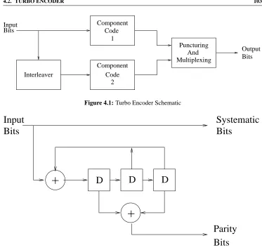
4.2

Turbo Encoder

(23)

Bits

Input Component

Code 1

Interleaver

2 Code

Component Multiplexing And Puncturing

[image:23.612.123.496.87.443.2]

Output Bits

Figure 4.1: Turbo Encoder Schematic

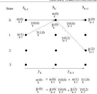
Input

Bits

Systematic

Bits

+

D

Bits

Parity

Figure 4.2: Recursive Systematic Convolutional (RSC) Encoder

it is possible to achieve good performance using a structure like that seen in Figure 4.1 with the aid of other components codes, such as for example block codes [68, 123]. Furthermore, it is also possible to employ more than two component codes. However, in this chapter we concentrate entirely on the standard turbo encoder structure using two RSC codes. Turbo codes using block codes as component codes are described in Chapter 6.

(24)

Decoder Component

Interleaver

Interleaver Soft

Channel

Inputs Parity 1

Parity 2 Systematic

De-Interleaver

-+

+

-Figure 4.3: Turbo Decoder Schematic

paper [21], but the dramatic improvement in performance that turbo codes gave arose because of the interleaver used between the encoders, and because recursive codes were used as the component codes. Recently theoretical paper have been published [65, 66] which try to ex-plain the remarkable performance of turbo codes. It appears that turbo codes can be thought of as having a performance gain proportional to the interleaver length used. However the decoding complexity per bit does not depend on the interleaver length. Therefore extremely good performance can be achieved with reasonable complexity by using very long inter-leavers. However for many important applications, such as speech transmission, extremely long frame lengths are not practical because of the delays they result in. Therefore in this chapter we have also investigated the use of turbo codes in conjunction with short frame lengths of the order of 100 bits.

4.3

Turbo Decoder

4.3.1

Introduction

(25)

described in Sections 4.3.6 and 4.3.3, respectively.

The decoder of Figure 4.3 operates iteratively, and in the first iteration the first compo-nent decoder takes channel output values only, and produces a soft output as its estimate of the data bits. The soft output from the first encoder is then used as additional information for the second decoder, which uses this information along with the channel outputs to calculate its estimate of the data bits. Now the second iteration can begin, and the first decoder decodes the channel outputs again, but now with additional information about the value of the input bits provided by the output of the second decoder in the first iteration. This additional infor-mation allows the first decoder to obtain a more accurate set of soft outputs, which are then used by the second decoder as a-priori information. This cycle is repeated, and with every it-eration the Bit Error Rate (BER) of the decoded bits tends to fall. However the improvement in performance obtained with increasing numbers of iterations decreases as the number of iterations increases. Hence, for complexity reasons, usually only about 8 iterations are used. Due to the interleaving used at the encoder, care must be taken to properly interleave and de-interleave the LLRs which are used to represent the soft values of the bits, as seen in Figure 4.3. Furthermore, because of the iterative nature of the decoding, care must be taken not to re-use the same information more than once at each decoding step. For this reason the concept of so-called extrinsic and intrinsic information was used in the original paper by Berou et al. describing iterative decoding of turbo codes [21]. These concepts and the reason for the subtraction circles shown in Figure 4.3 are described in Section 4.3.4.

Other, non-iterative, decoders have been proposed [124,125] which give optimal decoding of turbo codes. However the improvement in performance over iterative decoders was found to be only about 0.35 dB, and they are hugely complex. Therefore the iterative scheme shown in Figure 4.3 is commonly used. We now proceed with describing the concepts and algorithms used in the iterative decoding of turbo codes, commencing with the portrayal of logarithmic likelihood ratios.

4.3.2

Log Likelihood Ratios

The concept of Log Likelihood Ratios (LLRs) was shown by Robertson [126] to simplify the passing of information from one component decoder to the other in the iterative decoding of turbo codes, and so is now widely used in the turbo coding literature. The LLR of a data bit

u

kis denoted as L(u

k

)and is defined to be merely the log of the ratio of the probabilities of the bit taking its two possible values, ie:

L(u k

),ln

P(u k

=+1) P(u

k

= 1)

: (4.1)

Notice that the two possible values for the bitu

kare taken to be

+1and 1, rather than1and 0. This definition of the two values of a binary variable makes no conceptual difference, but it slightly simplifies the mathematics in the derivations which follow. Hence this convention is used throughout this chanpter. Figure 4.4 shows howL(u

k

)varies as the probability of u

k

=+1varies. It can be seen from this figure that the sign of the LLRL(u k

)of a bitu k will indicate whether the bit is more likely to be+1or 1, and the magnitude of the LLR gives an indication of how likely it is that the sign of the LLR gives the correct value ofu

k. When the LLRL(u

k

)0, we haveP(u k

=+1)P(u k

(26)

0.0 0.1 0.2 0.3 0.4 0.5 0.6 0.7 0.8 0.9 1.0

Prob (uk=+1)

-6 -4 -2 0 2 4 6

LLR(u

k

)

Figure 4.4: Log Likelihood RatioL(uk)Versus the Probability ofuk=+1

certain about the value ofu

k. Conversely, when L(u

k

) >> 0, we haveP(u k

=+1) >> P(u

k

= 1)and we can be almost certain thatu k

=+1. Given the LLRL(u

k

), it is possible to calculate the probability thatu k

=+1oru k

= 1

as follows. Remembering thatP(u k

= 1)=1 P(u

k

=+1), and taking the exponent of both sides in Equation 4.1 we can write:

e L(uk)

= P(u

k =+1)

1 P(u

k =+1)

; (4.2)

so

P(u k

=+1) =

e L(u

k ) 1+e

L(u k

)

=

1 1+e

L(u k

)

: (4.3)

Similarly

P(u k

= 1) =

1 1+e

+L(u k

)

= e

L(u k

) 1+e

L(u k

)

; (4.4)

and hence we can write

P(u k

=1)=

e

L(uk)=2 1+e

L(u k

)

e L(u

k )=2

(27)

Notice that the bracketed term in this equation does not depend on whether we are interested in the probability that u

k

= +1 or 1, and so it can be treated as a constant in certain applications, such as in Section 4.3.3 where we use this equation in the derivation of the MAP algorithm.

As well as the LLRL(u k

)based on the unconditional probabilitiesP(u k

=1), we are also interested in LLRs based on conditional probabilities. For example, in channel coding theory we are interested in the probability that u

k

= 1 based, or conditioned, on some received sequencey, and hence we may use the conditional LLRL(u

k

jy), which is defined as

L(u k

jy),ln

P(u k

=+1jy) P(u

k

= 1jy)

: (4.6)

The conditional probabilitiesP(u k

= 1jy)are known as the a-posteriori probabilities of the decoded bitu

k, and it is these a-posteriori probabilities that our soft-in soft-out decoders described in later sections attempt to find.

Apart from the conditional LLRL(u k

jy)based on the a-posteriori probabilitiesP(u k

= 1jy), we will also use conditional LLRs based on the probability that the receiver’s matched filter output would bey

kgiven that the corresponding transmitted bit x

kwas either

+1or 1. This conditional LLR is written asL(y

k jx

k

)and is defined as:

L(y k

jx k

),ln

P(y k

jx k

=+1) P(y

k jx

k

= 1)

: (4.7)

Notice the conceptual difference between the definitions of L(u k

jy) in Equation 4.6 and L(y

k jx

k

)in Equation 4.7, despite these two conditional LLRs being represented with very similar notation. This contrast in the definitions of conditional LLRs is somewhat confusing, but since these definitions are widely used in the turbo coding literature, we have introduced them here.

If we assume that the transmitted bitx k

=1has been sent over a Gaussian or fading channel using BPSK modulation, then we can write for the probability of the matched filter outputy

kthat:

P(y k

jx k

=+1)= 1

p 2

exp

E b 2

2 (y

k a)

2

; (4.8)

whereE

bis the transmitted energy per bit,

2

is the noise variance andais the fading ampli-tude (we havea=1for non-fading AWGN channels). Similarly, we have

P(y k

jx k

= 1)=

1

p 2

exp

E b 2

2 (y

k +a)

2

: (4.9)

(28)

Equation 4.7 as

L(y k

jx k

) , ln

P(y

k jx

k =+1) P(y

k jx

k

= 1)

= ln exp

E b 2

2 (y

k a)

2

exp E

b 2

2 (y

k +a)

2

!

=

E b 2

2 (y

k a)

2

E b 2

2 (y

k +a)

2

= E

b 2

2 4ay

k

= L

c y

k

; (4.10)

where

L c

=4a E

b 2

2

(4.11)

is defined as the channel reliability value, and depends only on the SNR and fading amplitude of the channel. Hence, for BPSK over a (possibly fading) Gaussian channel, the conditional LLRL(y

k jx

k

), which is referred to as the soft output of the channel, is simply the matched filter outputy

kmultiplied by the channel reliability value L

c.

Having introduced log likelihood ratios, we now proceed to describe the operation of the Maximum A-Posteriori algorithm, which is one of the possible soft-in soft-out component decoders that can be used in an iterative turbo decoder.

4.3.3

The Maximum A-Posteriori Algorithm

4.3.3.1 Introduction and Mathematical Preliminaries

In 1974 an algorithm, which is known as the Maximum A-Posteriori (MAP) algorithm, was proposed by Bahl, Cocke, Jelinek and Raviv for estimating the a-posteriori probabilities of the states and the transitions of a Markov source observed, when subjected to memoryless noise. This algorithm has also become known as the BCJR algorithm, named after its inventors. They showed, how the algorithm could be used for decoding both block and convolutional codes. When employed for decoding convolutional codes, the algorithm is optimal in terms of minimising the decoded bit error rate, unlike the Viterbi algorithm [18], which minimises the probability of an incorrect path through the trellis being selected by the decoder. Thus the Viterbi algorithm can be thought of as minimising the number of groups of bits associated with these trellis paths, rather than the actual number of bits, which are decoded incorrectly. Nevertheless, as stated by Bahl et al. in [20], in most applications the performance of the two algorithms will be almost identical. However the MAP algorithm examines every possible path through the convolutional decoder trellis and therefore initially seemed to be unfeasibly complex for application in most systems. Hence it was not widely used before the discovery of turbo codes.

(29)

this seminal paper. Since then much work has been done to reduce the complexity of the MAP algorithm to a reasonable level. In this section we describe the theory behind the MAP algorithm as used for the soft output decoding of the component convolutional codes of turbo codes. Throughout our work it is assumed that binary codes are used.

We use Bayes’ rule repeatedly throughout this section. This rule gives the joint probability ofaandb,P(a^b), in terms of the conditional probability ofagivenbas

P(a^b)=P(ajb)P(b): (4.12)

A useful consequence of Bayes’ rule is that:

P(fa^bgjc)=P(ajfb^cg)P(bjc); (4.13)

which can be derived from Equation 4.12 by consideringxa^bandy b^cas follows. From Equation 4.12 we can write

P(fa^bgjc) P(xjc)=

P(x^c) P(c)

=

P(a^b^c) P(c)

P(a^y) P(c)

=

P(ajy)P(y) P(c)

P(ajfb^cg)

P(b^c) P(c)

= P(ajfb^cg)P(bjc): (4.14)

The MAP algorithm gives, for each decoded bitu

k, the probability that this bit was +1 or 1, given the received symbol sequencey. As explained in Section 4.3.2 this is equivalent to finding the a-posteriori LLRL(u

k

jy), where

L(u k

jy)=ln

P(u k

=+1jy) P(u

k

= 1jy)

: (4.15)

Bayes’ rule allows us to rewrite this equation as

L(u k

jy)=ln

P(u k

=+1^y) P(u

k

= 1^y)

: (4.16)

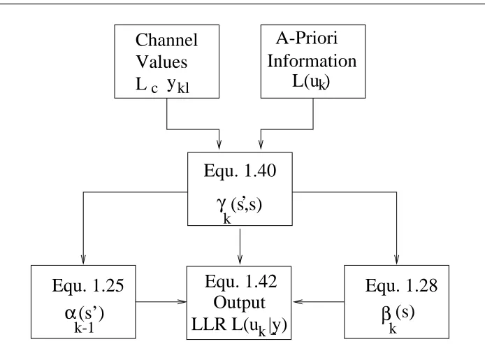
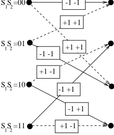
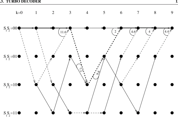
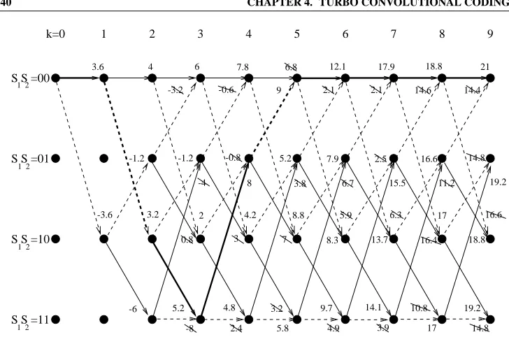
Let us now consider Figure 4.5 showing the transitions possible for theK = 3RSC code shown in Figure 4.2, which we have used for the component codes in most of our work. For thisK=3code there are four states, and as it is a binary code for each state two transitions are possible – one if the input bit is 1(shown as a solid line), and one if the input bit is a+1 (shown as a dashed line). It can be seen from Figure 4.5 that if the previous stateS

k 1and the present stateS

kare known, then the value of the input bit u

k, which caused the transition between these two states, will be known. Hence the probability thatu

k

=+1is equal to the probability that the transition from the previous stateS

k 1to the present state S

k is one of the set of four possible transitions that can occur whenu

k

(30)

S S

k-1 k

+1 -1

+1

-1

Figure 4.5: Possible Transitions inK=3 RSC Component Code

y

- j<k - ky - j>ky

S_k-3 S_k-2 S_k-1 S_k S_k+1

α

k-1

γ(s’,s)

k βk(s)

(s’)

s’

s

Figure 4.6: MAP Decoder Trellis forK=3RSC Code

have occured at the encoder), and so the probability that any one of them occurs is equal to the sum of their individual probabilities. Hence we can rewrite Equation 4.16 as

L(u k

jy)=ln 0 B B B B @

X

(s;s)) u

k =+1

P(S k 1

=s^S k

=s^y)

X

(s;s)) u

k = 1

P(S k 1

=s^S k

=s^y) 1 C C C C A

; (4.17)

where(s;s) ) u k

= +1is the set of transitions from the previous stateS k 1

=sto the present stateS

k

=sthat can occur if the input bitu k

=+1, and similarly for(s;s))u k

= 1. For brevity we shall writeP(S

k 1

=s^S k

=s^y)asP(s^s^y).

(31)

received codeword associated with the present transitiony k

, the received sequence prior to the present transitiony

j<k

and the received sequence after the present transitiony j>k

. This split is shown in Figure 4.6, again for the example of ourK=3RSC component code shown in Figure 4.2. We can thus write for the individual probabilitiesP(s^s^y)

P(s^s^y)=P(s^s^y j<k ^y k ^y j>k ): (4.18)

Using Bayes’ rule ofP(a^b)=P(ajb)P(b)and the fact that if we assume that the chan-nel is memoryless, then the future received sequencey

j>k

will depend only on the present statesand not on the previous statesor the present and previous received channel sequences y

k andy

j<k

, we can write

P(s^s^y) = P(y j>k

jfs^s^y j<k

^y k

g)P(s^s^y j<k

^y k

) = P(y

j>k

js)P(s^s^y j<k

^y k

): (4.19)

Again, using Bayes’ rule and the assumption that the channel is memoryless, we can expand Equation 4.19 as follows:

P(s^s^y) = P(y j>k

js)P(s^s^y j<k

^y k

) = P(y

j>k

js)P(fy k

^sgjfs^y j<k

g)P(s^y j<k

) = P(y

j>k

js)P(fy k

^sgjs)P(s^y j<k ) = k (s) k

(s;s) k 1

(s); (4.20)

where

k 1

(s)=P(S k 1

=s^y j<k

) (4.21)

is the probability that the trellis is in statesat timek 1and the received channel sequence up to this point isy

j<k

, as visualised in Figure 4.6,

k

(s)=P(y j>k

jS k

=s) (4.22)

is the probability that given the trellis is in state s at time k the future received channel sequence will bey

j>k

, and lastly

k

(s ;s)=P(fy k

^S k

=sgjS k 1

=s) (4.23)

is the probability that given the trellis was in statesat timek 1, it moves to statesand the received channel sequence for this transition isy

k .

Equation 4.20 shows that the probabilityP(s^s^y), that the encoder trellis took the transition from stateS

k 1

=sto stateS k

=sand the received sequence isy, can be split into the product of three terms –

k 1 (s),

k

(s;s)and k

(s). The meaning of these three probability terms is shown in Figure 4.6, for the transition S

k 1

= stoS k

= sshown by the bold line in this figure. The MAP algorithm finds

k

(s)and k

(s)for all statess throughout the trellis, ie fork=0;1N 1, and

k

(32)

α

k-1

(0)

β

k+1

(0)

y

- k

γ

(0,0)

k

α

k

(0)

α

k-1

(1)

γ

(1,0)

k

β

(0)

k

β

(2)

k+1

γ

(0,2)

k+1

α

k

(0)

β

(0)

k

α

k-1

(0)

β

(0)

k+1

γ

(0,0)

k

β

(2)

k+1

γ

k+1

(0,2)

γ

(0,0)

k+1

α

k-1

(1)

γ

k

(1,0)

γ

(0,0)

k+1

S

_k-1

S

_k

S

_k+1

1

0

2

3

State

y

- k+1

=

+

[image:32.612.119.434.89.394.2]

+

Figure 4.7: Recursive Calculation ofk(0)andk(0)

stateS k 1

=sto stateS k

=s, again fork =0;1N 1. These values are then used to find the probabilitiesP(S

k 1

=s^S k

=s^y)of Equation 4.20, which are then used in Equation 4.17 to give the LLRsL(u

k

jy)for each bitu

k.These operations are summarised in the flowchart of Figure 4.8. We now describe how the values

k (s),

k

(s)and k

(s;s)can be calculated.

4.3.3.2 Forward Recursive Calculation of the k

(s)Values Consider first

k

(s). From the definition of k 1

(s)in Equation 4.21 we can write

k

(s) = P(S k

=s^y j<k +1

) = P(s^y

j<k ^y

k )

= X

alls

P(s^s^y j<k

^y k

); (4.24)

where in the last line we split the probabilityP(s^y y<k +1

(33)

that the channel is memoryless again, we can proceed as follows:

k

(s) =

X

alls

P(s^s^y j<k ^y k ) = X

alls

P(fs^y k

gjfs^y j<k

g)P(s^y j<k

)

= X

alls

P(fs^y k

gjs)P(s^y j<k

)

= X

alls

k

(s ;s) k 1

(s): (4.25)

Thus, once the k

(s;s)values are known, the k

(s)values can be calculated recursively. Assuming that the trellis has the initial stateS

0

=0, the initial conditions for this recursion are

0

(S 0

=0) = 1

0

(S 0

=s) = 0 foralls6=0: (4.26) Figure 4.7 shows an example of how one

k

(s)value, fors =0, is calculated recursively using values of

k 1

(s)and k

(s;s)for our exampleK =3RSC code. Notice that, as we are considering a binary trellis, only two previous states,S

k =1

=0andS k 1

=1, have paths to the stateS

k

=0. Therefore k

(s;s)will be non-zero only fors=0ors=1and hence the summation in Equation 4.25 is over only two terms.

4.3.3.3 Backward Recursive Calculation of the k

(s)Values The values of

k

(s)can similarly be calculated recursively as shown below. From the defini-tion of

k

(s)in Equation 4.22, we can write k 1

(s)as

k 1

(s)=P(y j>k 1

jS k 1

=s); (4.27)

and again splitting a single probability into the sum of joint probabilities and using the deriva-tion from Bayes’ rule in Equaderiva-tion 4.13, as well as the assumpderiva-tion that the channel is memo-ryless, we have:

k 1

(s) = P(y j>k 1 js) = X alls P(fy j>k 1 ^sgjs)

= X alls P(fy k ^y j>k ^sgjs)

= X

alls P(y

j>k

jfs^s^y k

g)P(fy k

^sgjs)

= X

alls P(y

j>k

js)P(fy k

^sgjs)

= X k (s) k

(34)

Thus, once the values k

(s ;s)are known, a backward recursion can be used to calculate the values of

k 1

(s) from the values of k

(s)using Equation 4.28. Figure 4.7 again shows an example of how the

k

(0)value is calculated recursively using values of k +1

(s)and

k +1

(0;s)for our exampleK=3RSC code. The initial conditions which should be used for

N

(s)are not as clear as for 0

(s). From Equation 4.22

k

(s)is the probability that the future received sequence isy j>k

, given that the present state iss. For the last stage in the trellis however, ie whenk = N, there is no future received sequence, and hence it is not clear what the initial valuesB

N

(s)should be set to. Berrou et al. [21] used the initial values

N

(0)=1and N

(s)=0for alls6=0for a trellis terminated in the all zero state, and in [126] the initial conditions for an unterminated trellis were given by Robertson as

N

(s) = N

(s)for alls. However, as pointed out by Breiling [127], if we consider

N 1

(s)from Equation 4.22 we have

N 1

(s) = P(y N

js) =

X

alls P(fy

N ^sgjs)

= X

alls

N

(s;s) (4.29)

and from the backward recursion for k 1

(s )in Equation 4.28 we have

N 1

(s )= X

alls

N (s)

N

(s;s): (4.30)

For both Equation 4.29 and Equation 4.30 to be satisfied, we must have

N

(s)=1 foralls: (4.31)

If the trellis is terminated, so that only the final stateS N

=0is possible, this can be taken into account in the backward recursive calculation of the

k

(s)values through the k

(s ;s) values. In a terminated trellis for the lastK 1transitions, whereKis the constraint length of the convolutional code, for each statesonly one transition (the one which takes the trellis towards the all-zero state) will be possible. Hence

k

(s;s)=P(fy k

^S k

=sgjS k 1

=s) will be zero for all values ofsexcept one, and with the initial values

N

(s)=1the correct values of

N 1 (s);

N 2

(s);

N K+1 will be calculated through Equation 4.28. Thus theory indicates that we should use

N

(s)=1for allsand account for the trellis termination by setting the values of

k

(s;s)to zero for all transitions that are not possible due to trellis termination. However the same result can be achieved using values of

N

(0) = 1and

N

(s) = 0forsneq0, as suggested by Berrou et al. [21], and calculating k

(s;s)values in the same way as for all other transitions (i.e. directly from the channel inputs - see next section). This second method is simpler to implement and hence it is more commonly used in practice.

4.3.3.4 Calculation of the k

(s;s)Values We now consider how the

k

(s;s)values in Equation 4.20 can be calculated from the received channel sequence. Using the definition of

k

(35)

Bayes’ rule given in Equation 4.13 we have

k

(s;s) = P(fy k

^sgjs) = P(y

k

jfs^sg)P(sjs) = P(y

k

jfs^sg)P(u k

); (4.32)

whereu

kis the input bit necessary to cause the transition from state S

k 1

=sto stateS k

=s, andP(u

k

)is the a-priori probability of this bit. From Equation 4.5 this can be written as

P(u k ) = e L(u k )=2 1+e

L(u k ) e (ukL(uk)=2) = C (1) L(uk) e (ukL(uk)=2) ; (4.33)

where, as stated before,

C (1) L(uk) = e L(u k )=2 1+e

L(u k

)

(4.34)

depends only on the LLRL(u k

)and not on whetheru kis

+1or 1. The first term in second and third lines of Equation 4.32,P(y

k

jfs^sg), is equivalent toP(y

k jx

k

), wherex k

is the transmitted codeword associated with the transition from state

S k 1

=sto stateS k

=s. Again assuming the channel is memoryless we can write

P(y k

jfs^sg)P(y k jx k )= n Y l=1 P(y k l jx k l ); (4.35) wherex k l and

y

k l are the individual bits within the transmitted and received codewords y

k andx

k

, andnis the number of these bits in each codewordy k

or x k

. Assuming that the transmitted bitsx

k l have been transmitted over a Gaussian channel using BPSK, so that the transmitted symbols are either+1or 1, we have forP(y

k l jx k l ) P(y k l jx k l )= 1 p 2 exp E b 2 2 (y k l ax k l ) 2 ; (4.36) whereE

bis the transmitted energy per bit,

2

is the noise variance andais the fading ampli-tude (a=1 for non-fading AWGN channels). Upon substituting Equation 4.36 in Equation 4.35 we have

P(y k

(36)

where C (2) y k = 1 ( p 2) n exp E b 2 2 n X l=1 y 2 k l ! (4.38)

depends only on the channel SNR and on the magnitude of the received sequencey k , while C (3) x k = exp E b 2 2 a 2 n X l=1 x 2 k l ! = exp E b 2 2 a 2 n (4.39)

depends only on the channel SNR and on the fading amplitude. Hence we can write for

k

(s;s)

k

(s ;s) = P(u k

)P(y k

jfs^sg)

= Ce

(ukL(uk)=2) exp E b 2 2 2a n X l=1 y k l x yl !

= Ce

(u k L(u k )=2) exp L c 2 n X l=1 y k l x yl ! ; (4.40) where

C=C (1) L(uk) C (2) y k C (3) x k : (4.41)

The termCdoes not depend on the sign of the bitu

k or the transmitted codeword x

k and so is constant over the summations in the numerator and denominator in Equation 4.17 and cancels out.

From Equations 4.17 and 4.20 we can write for the conditional LLR ofu

k, given the received sequencey

k ,

L(u k

jy) = ln 0 B B B B @ X (s;s)) u k =+1 P(S k 1

=s^S k

=s^y)

X (s;s)) u k = 1 P(S k 1

=s^S k

=s^y) 1 C C C C A = ln 0 B B B B @ X (s;s)) u k =+1 k 1 (s) k

(s;s) k (s) X (s;s)) u k = 1 k 1 (s) k

(s ;s) k (s) 1 C C C C A : (4.42)

It is this conditional LLRL(u k

(37)

L(u )

k

(s,s)

’

Channel

Values

L

c

y

kl

γ

k

Equ. 1.40

Equ. 1.28

β

(s)

k

Equ. 1.25

(s’)

α

k-1

Information

A-Priori

[image:37.612.140.487.92.338.2]

Equ. 1.42

Output

LLR L(u |y)

k

Figure 4.8: Summary of the Key Operations in the MAP Algorithm

4.3.3.5 Summary of the MAP Algorithm

¿From the description given above, we see that the MAP decoding of a received sequencey to give the a-posteriori LLRL(u

k

jy)can be carried out as follows. As the channel values y

k lare received, they and the a-priori LLRs L(u

k

)(which are provided in an iterative turbo decoder by the other component decoder – see Section 4.3.4) are used to calculate

k (s;s) according to Equation 4.40. The constantCcan be omitted from the calculation of

k (s;s), as it will cancel out in the ratio in Equation 4.42. As the channel values y

k l are received, and the

k

(s;s)values are calculated, the forward recursion from Equation 4.25 can be used to calculate

k

(s ;s). Once all the channel values have been received, and k

(s ;s)has been calculated for allk = 1;2N, the backward recursion from Equation 4.28 can be used to calculate the

k

(s;s)values. Finally all the calculated values of k

(s;s), k

(s;s)and

k

(s;s)are used in Equation 4.42 to calculate the values ofL(u k

jy). These operations are summarised in the flowchart of Figure 4.8. Care must be taken to avoid numerical underflow problems in the recursive calculation of

k

(s ;s) and k

(s;s), but such problems can be avoided by careful normalisation of these values. Such normalisation cancels out in the ratio in Equation 4.42 and so causes no change in the LLRs produced by the algorithm.

The MAP algorithm is, in the form described in this section, extremely complex due to the multiplications needed in Equations 4.25 and 4.28 for the recursive calculation of

k

(s;s)and k

(s;s), the multiplications and exponential operations required to calculate

k

(s;s)using Equation 4.40, and the multiplication and natural logarithm operations required to calculateL(u

k

(38)

the numerical problems described above. We will first describe the principles behind the iterative decoding of turbo codes, and how the MAP algorithm described in this section can be used in such a scheme, before detailing the Log-MAP algorithm.

4.3.4

Iterative Turbo Decoding Principles

4.3.4.1 Turbo Decoding Mathematical Preliminaries

In this section we explain the concepts of extrinsic and intrinsic information as used by Berrou el al [21], and highlight how the MAP algorithm described in the previous section, and other soft-in soft-out decoders, can be used in the iterative decoding of turbo codes.

Consider first the expression for k

(s;s)in Equation 4.40, which is restated here for convenience

k

(s;s)=Ce (u

k L(u

k )=2)

exp L

c 2

n X

l=1 y

k l x

yl !

: (4.43)

As we are dealing with systematic codes one of thentransmitted bits will be the systematic bitu

k. If we assume that this systematic bit is the first of the

ntransmitted bits then we will havex

k 1 =u

k, and we can rewrite Equation 4.43 as

k

(s ;s) = Ce

(ukL(uk)=2) exp

L

c 2

y k s

u k

exp

L c 2

n X

l=2 y

k l x

yl !

= Ce

(u k

L(u k

)=2) exp

L

c 2

y k s

u k

k

(s;s); (4.44)

wherey

k sis the received version of the transmitted systematic bit x

k 1 =u

kand

k

(s ;s)=exp L

c 2

n X

l=2 y

k l x

yl !

: (4.45)

Using Equation 4.44 and remembering that in the numerator we haveu k

=+1for all terms in the summation, whereas in the denominator we haveu

k

(39)

as

L(u k

jy) = ln 0 B B B B @ X (s;s)) u k =+1 k 1 (s) k

(s;s) k (s) X (s;s)) u k = 1 k 1 (s) k

(s ;s) k (s) 1 C C C C A = ln 0 B B B B @ X (s;s)) u k =+1 k 1

(s)e +L(u k )=2 e +L c y k s =2 k

(s;s) k (s) X (s;s)) u k = 1 k 1

(s )e L(u k )=2 e L c y k s =2 k

(s;s) k (s) 1 C C C C A = L(u k )+L

c y k s +ln 0 B B B B @ X (s ;s)) u k =+1 k 1 (s) k

(s;s) k

(s)

X (s ;s)) u k = 1 k 1 (s) k

(s;s) k (s) 1 C C C C A = L(u k )+L

c y k s +L e (u k ); (4.46) where L e (u k

)=ln 0 B B B B @ X (s;s)) u k =+1 k 1 (s) k

(s;s) k (s) X (s;s)) u k = 1 k 1 (s) k

(s;s) k (s) 1 C C C C A : (4.47)

Thus we can see that the a-posteriori LLRL(u k

jy)calculated with the MAP algorithm can be thought of as comprising of three terms –L(u

k ),L

c y

k s and L

e (u

k

). The a-priori LLR termL(u

k

)comes fromP(u k

)in the expression for the branch transition probability k

(s;s) in Equation 4.32. This probability should come from an independent source and is called the a-priori probability of thek’th bit being+1or 1. In most cases we will have no independent or a-priori knowledge of the likely value of the bitu

k, and so the a-priori LLR L(u

k )will be zero, corresponding to an a-priori probability P(u

k

) = 0:5. However, in the case of an iterative turbo decoder, each component decoder can provide the other decoder with an estimate of the a-priori LLRL(u

k

), as described later. The second termL

c y

k sin Equation 4.46 is the soft output of the channel for the system-atic bitu

k, which was directly transmitted across the channel and received as y

k s. When the channel SNR is high, the channel reliability valueL

c of Equation 4.11 will be high and this systematic bit will have a large influence on the a-posteriori LLRL(u

k

jy). Conversely, when the channel is poor andL

cis low, the soft output of the channel for the received systematic bity

k swill have less impact on the a-posteriori LLR delivered by the MAP algorithm. The final term in Equation 4.46,L

e (u

k

), is derived, using the constraints imposed by the code used, from the a-priori information sequenceL(u

n

)and the received channel informa-tion sequencey, excluding the received systematic bity

k sand the a-priori information L(u

k ) for the bitu

k. Hence it is called the extrinsic LLR for the bit u

(40)

extrinsic information from a MAP decoder can be obtained by subtracting the a-priori infor-mationL(u

k

)and the received systematic channel inputL c

y

k sfrom the soft output L(u

k jy) of the decoder. This is the reason for the subtraction paths shown in Figure 4.3. Equations similar to Equation 4.46 can be derived for the other component decoders which can be used in iterative turbo decoding.

Notice that the expression for the branch transition probabilities k

(s;s)in Equation 4.40 uses the a-priori informationL(u

k

)and all nbits, including the systematic bity

k s, of the received codewordy

k

. These branch transition probabilities are used in the recursive cal-culations of

k

(s)and k

(s)in Equations 4.25 and 4.28 and so, as these terms appear in Equation 4.47 forL

e (u

k

), it might seem that the received systematic bity

k sand the a-priori informationL(u

k

)for the bitu

k appear indirectly in the extrinsic output L

e (u

k

). However careful examination of Equation 4.47 shows that for the bitu

k we use the values of

k 1 (s) and

k

(s). From Equations 4.25 and 4.28 for the recursive calculation of the these values we see that the branch transition probabilities

n

(s;s)for1nk 1andk+1nNwill be used to calculate the

k 1

(s)and k

(s)values. Notice however that the branch transition probability

k

(s;s), for the transition associated with the bitu

k, is not used. Hence L

e (u

k ) uses the values of the branch transition probabilities

n

(s ;s)for all the branches except the k’th branch. Therefore, although it does depend on all the other a-priori information terms L(u

n

) and received systematic bits, the termL e

(u k

) really is independent of the a-priori informationL(u

k

)and the received systematic bity

k s, and so can justifiably be called the extrinsic LLR for the bitu

k.

We summarise below what is meant by the terms a-priori, a-posteriori and extrinsic infor-mation which we use throughout this treatise.

a-priori The a-priori information about a bit is information known before decoding starts, from a source other than the received sequence or the code constraints. It is also some-times referred to as intrinsic information to contrast with the extrinsic information de-scribed next.

extrinsic The extrinsic information about a bitu

kis the information provided by a decoder based on the received sequence and on a-priori information excluding the received sys-tematic bity

k sand the a-priori information L(u

k

)for the bitu

k. Typically the compo-nent decoder provides this information using the constraints imposed on the transmitted sequence by the code used. It processes the received bits and a-priori information sur-rounding the systematic bitu

k, and uses this information and the code constraints to provide information about the value of the bitu

k.

a-posteriori The a-posteriori information about a bit is the information that the decoder gives taking into account all available sources of information aboutu

k. It is the a-posteriori LLR, ieL(u

k

jy), that the MAP algorithm gives as its output.

4.3.4.2 Iterative Turbo Decoding

(41)

Decoder Component Decoder Component Interleaver k L(u )

k L(u )

De-Interleaver Interleaver

k L (u )_e

-+ + -k L(u |y)

k L(u |y) L y_{c ks}

L y_{c ks} Soft

Channel Inputs

L y_{c kl} L y c kl Parity 1

Parity 2 Systematic

Figure 4.9: Turbo Decoder Schematic

Consider initially the first component decoder in the first iteration. This decoder receives the channel sequenceL

c y

(1)

containing the received versions of the transmitted systematic bits,L

c y

k s, and the parity bits, L

c y

k l, from the first encoder. Usually, to obtain a half-rate code, half of these parity bits will have been punctured at the transmitter, and so the turbo decoder must insert zeros in the soft channel outputL

c y

k l for these punctured bits. The first component decoder can then process the soft channel inputs and produce its estimate

L 11

(u k

jy)of the conditional LLRs of the data bitsu k,

k =1;2N. In this notation the subscript 11 inL

11 (u

k

jy)indicates that this is the a-posteriori LLR in the first iteration from the first component decoder. Note that in this first iteration the first component decoder will have no a-priori information about the bits, and henceL(u

k

)in Equation 4.40 giving k

(s;s) will be zero, corresponding to an a-priori probability of 0.5.

Next the second component decoder comes into operation. It receives the channel se-quence L

c y

(2)

containing the interleaved version of the received systematic bits, and the parity bits from the second encoder. Again, the turbo decoder will have to insert zeros into this sequence, if the parity bits generated by the encoder are punctured before transmission. However now, in addition to the received channel sequenceL

c y

(2)

, the decoder can use the conditional LLR L

11 (u

k

jy) provided by the first component decoder to generate a-priori LLRsL(u

k

)to be used by the second component decoder. Ideally these a-priori LLRsL(u k

) would be completely independent from all the other information used by the second com-ponent decoder. As can be seen in Figure 4.9 in iterative turbo decoders the extrinsic infor-mationL

e (u

k

)from the other component decoder is used as the a-priori LLRs, after being interleaved to arrange the decoded data bitsuin the same order as they were encoded by the second encoder. Again, according to Equation 4.46, the reason for the subtraction paths shown in Figure 4.9 is that the a-posteriori LLRs from one decoder have the systematic soft channel inputsL

c y

k sand the a-priori LLRs L(u

k

)(if any were available) subtracted to yield the extrinsic LLRsL

e (u

k

)which are then used as a-priori LLRs for the other component decoder. The second component decoder thus uses the received channel sequence L

c y

(2) and the a-priori LLRsL(u

k

)(derived by interleaving the extrinsic LLRsL e

(u k

)of the first component decoder) to produce its a-posteriori LLRsL

12 (u

k

(42)

For the second iteration the first component encoder again processes its received channel sequenceL

c y

(1)

, but now it also has a-priori LLRsL(u k

)provided by the extrinsic portion L

e (u

k

)of the a-posteriori LLRs L 12

(u k

jy)calculated by the second component encoder, and hence it can produce an improved a-posteriori LLRL

21 (u

k

jy). The second iteration then continues with the second component decoder using the improved a-posteriori LLRs

L 21

(u k

jy)from the first encoder to derive, through Equation 4.46, improved a-priori LLRs L(u

k

)which it uses in conjunction with its received channel sequenceL c

y (2)

to calculate

L 22

(u k

jy).

This iterative process continues, and with each iteration on average the BER of the de-coded bits will fall. However, as will be seen in Figure 4.20, the improvement in performance for each additional iteration carried out falls as the number of iterations increases. Hence for complexity reasons usually only about eight iterations are carried out, as no significant improvement in performance is obtained with a higher number of iterations. This is the ar-rangement we have used in most of our simulations, ie the decoder carries out a fixed number of iterations. However it is possible to use a variable number of iterations up to a maximum, with some termination criterion used to decide when it is deemed that further iterations will produce marginal gain. This allows the average number of iterations, and so the average complexity of the decoder, to be dramatically reduced [68] with only a small degradation in performance. Suitable termination criteria have been found to be the so-called cross-entropy of the outputs from the two component decoders [68], and the variance of the a-posteriori LLRsL(u

k

jy)of a component decoder [126].

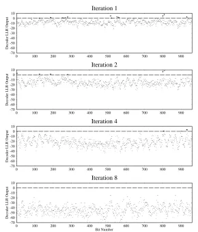
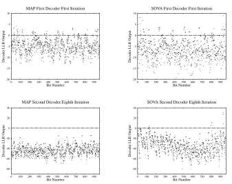
Figure 4.10 shows how the a-posteriori LLRsL(u k

jy)output from the component de-coders in an iterative decoder vary with the number of iterations used. The output from the second component decoder is shown after 1,2,4 and 8 iterations. The input sequence of the encoder consisted entirely of logical 0’s, and consequently the negative a-posteriori LLR

L(u k

jy)values correspond to a correct hard decision, while the positive values to an incor-rect hard decision. The input sequence was coded using a turbo encoder with two constraint length 3 recursive convolutional codes, and a block interleaver with 31 rows and 31 columns. This turbo encoder is used in the majority of our investigations and its performance is char-acterised in Section 4.4. The encoded bits were transmitted over an AWGN channel at a channel SNR of -1 dB, and then decoded using an iterative turbo decoder using the MAP al-gorithm. It can be seen that as the number of iterations used increases, the number of positive a-posteriori LLRL(u

k

jy)values, and hence the BER, decreases until after eight iterations there are no incorrectly decoded values. Furthermore, as the number of iterations increases, the decoders become more certain about the value of the bits and hence the magnitudes of the LLRs gradually become larger. The erroneous decisions in the figure appear in bursts, since deviating from the error-free path trellis path typically inflicts several bi