Investigation of structure and disorder in inorganic solids using solid state NMR

25=/9;21,;265 60 9;8<-;<8/ ,5. .2968./8 25 25681,52- 9632.9 <9251 9632.!9;,;/ 548

4>MOFJ 8K?BMO 4FO@EBHH

, ;EBNFN 9P?IFOOBA CKM OEB .BDMBB KC 7E. >O OEB

<JFQBMNFOT KC 9O" ,JAMBRN

&$%'

0PHH IBO>A>O> CKM OEFN FOBI FN >Q>FH>?HB FJ 8BNB>M@E+9O,JAMBRN*0PHH;BSO

>O*

EOOL*##MBNB>M@E!MBLKNFOKMT"NO!>JAMBRN">@"PG#

7HB>NB PNB OEFN FABJOFCFBM OK @FOB KM HFJG OK OEFN FOBI* EOOL*##EAH"E>JAHB"JBO#%$$&'#''()

Investigation of Structure and Disorder in

Inorganic Solids Using Solid-State NMR

Martin Robert Mitchell

This thesis is submitted in partial fulfilment for

the degree of PhD at the University of St Andrews

Declaration

I, Martin Robert Mitchell, hereby certify that this thesis, which is approximately 55000 words in length, has been written by me, that it is the record of work carried out by me and that it has not been submitted in any previous application for a higher degree.

I was admitted as a research student in September, 2008 and as a candidate for the degree of PhD in September, 2009; the higher study for which this is a record was carried out in the University of St Andrews between 2008 and 2012.

Date Signature of candidate

regulations of the University Library for the time being in force, subject to any copyright vested in the work not being affected thereby. I also understand that the title and the abstract will be published, and that a copy of the work may be made and supplied to any bona fide library or research worker, that my thesis will be electronically accessible for personal or research use unless exempt by award of an embargo as requested below, and that the library has the right to migrate my thesis into new electronic forms as required to ensure continued access to the thesis. I have obtained any third-party copyright permissions that may be required in order to allow such access and migration, or have requested the appropriate embargo below.

The following is an agreed request by candidate and supervisor regarding the electronic publication of this thesis:

Access to printed copy and electronic publication of thesis through the University of St Andrews.

Acknowledgements

First and foremost, I would like to thank my supervisor, Dr Sharon Ashbrook, for her never-ending help, support and patience throughout the last four years. Special thanks must also go to Dr John Griffin and Dr Karen Johnston for their guidance and support.

I would also like to thank in no particular order Dr Donna Arnold, Dr Frédéric Blanc, Dr Diego Carnevale, Miss Rachael Crowe, Dr Dinu Igua, Dr Finlay Morrison, Dr Robin Orr, Professor Chris Pickard and Dr Karl Whittle for their help and contributions to my research. Additional thanks also goes to the past and present members of the Ashbrook group.

Finally, I would like to thank all of my friends, notably Ryan and Bobby, my girlfriend Heather, and my parents.

M. R. Mitchell, D. Carnevale, R. Orr, K. R. Whittle and S. E. Ashbrook, J. Phys. Chem. C., 2012, 116, 4273

M. R. Mitchell, S. W. Reader, K. E. Johnston, C. J. Pickard, K. R. Whittle and S. E. Ashbrook, Phys. Chem. Chem. Phys., 2011, 13, 488

1 Introduction 1

1.1 Thesis overview 1

2 Experimental techniques 5

2.1 Basic principles of NMR 5

2.1.1 Nuclear magnetism 5

2.1.2 The vector model 7

2.1.3 Fourier transformation 8

2.1.4 Density operator formalism 10

2.2 NMR interactions 11

2.2.1 Internal interactions 11

2.2.2 J-coupling 12

2.2.3 Chemical shielding and chemical shift anisotropy 13

2.2.4 Dipolar coupling 16

2.2.5 Quadrupolar coupling 18

2.3 Magic angle spinning 22

2.3.1 Orientation dependence of interactions 22 2.3.2 Effect of MAS on the CSA interaction 23

2.4.1 Spin echo 25

2.4.2 CPMG 26

2.4.3 INADEQUATE 28

2.5 Computational chemistry 30

2.5.1 Introduction 30

2.5.2 The Schrödinger equation 30

2.5.3 Density functional theory 31

2.5.4 Wavefunctions in a periodic system 32

2.5.5 Methodology of CASTEP 36

3 Pyrochlore and defect fluorite materials: Ceramics for the

encapsulation of nuclear waste 38

3.1 Materials 38

3.1.1 Pyrochlores 38

3.1.2 Defect fluorite 41

3.2 Immobilisation of radioactive cations in ceramic wasteforms 41

3.2.1 Background 41

3.2.2 Synroc 43

3.2.3 Radiation damage processes 44

3.3 Previous work 47 3.3.1 89Y solid-state NMR of Y2SnxTi2–xO7 47 3.3.2 89Y DFT calculations of Y2SnxTi2–xO7 51

3.3 Conclusions 60

4 Multinuclear solid-state NMR investigation of Y2SnxTi2–xO7 61

4.1 Introduction 61

4.2 Experimental methods 63

4.2.1 NMR spectroscopy 63

4.2.2 DFT calculations 64

4.2.3 Sample preparation 64

4.3 119Sn and 117Sn NMR investigation of Y2SnxTi2–xO7 65

4.3.1 119Sn and 117Sn MAS NMR spectra 65

4.3.2 119Sn 2D refocused-INADEQUATE spectra 66 4.3.3 Optimisation and evaluation of 119Sn DFT calculations 69 4.3.4 119Sn DFT calculations for the study of disordered

pyrochlores 74

4.3.5 Assignment of 119Sn NMR spectra 76

4.4 17O NMR investigation of Y2SnxTi2–xO7 81

4.4.1 Introduction and previous studies 81

4.4.2 17O NMR spectra 82

4.4.3 17O DFT and point charge calculations 83

4.4.4 17O NMR conclusions 85

4.5 47/49Ti NMR investigation of Y2SnxTi2–xO7 86

4.5.1 Introduction and previous studies 86

4.5.2 47/49Ti NMR spectra 87

4.5.3 47/49Ti DFT calculations 89

4.5.4 47/49Ti NMR conclusions 91

4.6 Conclusions 91

5 Application of the 2D CSA amplified-PASS (CAPASS) experiment

to 89Y NMR 93

5.1 Introduction 93

5.2 Experimental parameters 98

5.2.1 NMR spectroscopy 98

5.2.2 Sample preparation 99

5.3 Results and discussion 99

5.3.1 Accuracy of the measurement of the CSA using 89Y slow

train 104 5.3.3 Assessment of the CAPASS fitting procedure 110 5.3.4 Investigating CAPASS experimental parameters 113 5.3.5 Effects of varying rf field strength on CAPASS 119 5.3.6 Effect of pulse imperfections on CAPASS performance 121

5.4 Conclusions 128

6 89Y and 119Sn 2D CSA-amplified PASS (CAPASS) NMR

of Y2SnxTi2–xO7 129

6.1 Introduction 129

6.2 Experimental parameters 131

6.2.1 NMR spectroscopy 131

6.2.2 DFT calculations 132

6.2.3 Sample preparation 132

6.3 89Y NMR investigation of Y2SnxTi2–xO7 133

6.3.1 89Y DFT calculations 133

6.3.2 89Y CAPASS spectra 140

6.3.3 Assignment of 89Y NMR CAPASS spectra using DFT

calculations 146

6.3.5 89Y NMR conclusions 152

6.4 119Sn NMR investigation of Y2SnxTi2–xO7 153

6.4.1 119Sn DFT calculations 153

6.4.2 119Sn CAPASS spectra 155

6.4.3 119Sn NMR conclusions 159

6.5 Conclusions 159

7 Investigation of ordered and disordered phases in Y2SnxZr2–xO7

and Y2TixZr2–xO7 161

7.1 Introduction 161

7.2 Experimental parameters 165

7.2.1 NMR spectroscopy 165

7.2.2 DFT calculations 167

7.2.3 Sample preparation 167

7.3 89Y NMR investigation of Y2SnxZr2–xO7 168

7.3.1 89Y NMR spectra 168

7.3.2 89Y CAPASS of Y2Sn1.6Zr0.4O7 180

7.3.3 89Y DFT calculations 182

7.3.4 89Y NMR discussions and conclusions 189

7.4 119Sn NMR investigation of Y2SnxZr2–xO7 191

7.4.3 Sn NMR discussion and conclusions 200

7.5 91Zr NMR investigation of Y2SnxZr2–xO7 202

7.5.1 91Zr NMR introduction 202

7.5.2 Optimisation and testing of 91Zr DFT calculations 202

7.5.3 91Zr DFT calculations 204

7.5.4 91Zr NMR spectra 206

7.5.5 91Zr NMR conclusions 212

7.6 Discussion of Y2SnxZr2–xO7 213

7.6.1 Analysis of cation ordering 213

7.6.2 Analysis of anions/vacancies ordering 215

7.7 89Y NMR investigation of Y2TixZr2–xO7 220

7.7.1 89Y NMR spectra 220

7.7.2 89Y DFT calculations 222

7.7.3 Comparison of 89Y NMR of Y2TixZr2–xO7 and Y2SnxZr2–xO7 225

7.7.4 89Y NMR conclusions 226

7.8 Conclusions 227

8 Conclusions and future work 229

8.1 Conclusions 229

9 References 234

A Theory for MAS and spinning sidebands 251

A.1 Introduction 251

A.2 Describing the CSA 251

A.3 Effects of MAS on the CSA interaction 253

B Refocused-INADEQUATE phase cycling 257

C Geometry optimisations on Y2Sn2O7 259

D Theory for 2D CSA-amplified PASS (CAPASS) 263

B.1 A carousel of spins 263

Introduction

1.1 Thesis overview

The increasing use of nuclear power stations has resulted in an increasing amount of radioactive waste for which there is not yet a preferred mode for permanent storage. Additionally, silicate glasses, widely regarded as a first-generation wasteform, are not ideal for the encapsulation of radioactive waste as they suffer from numerous problems, such as low loading and corrosion when in contact with humidity. Therefore, research into the development of an improved second-generation wasteform is critical to the safe storage of radioactive waste. One of these proposed second-generation wasteforms is SYNROC-F, which contains large quantities of a titanate pyrochlore. The pyrochlore structure in particular has proved popular due to its higher waste loading and chemical durability, in comparison with silicate glasses. Other pyrochlores such as the zirconate and stannate pyrochlores, have additional benefits as a wasteform, as atomic displacement damage results in the formation of a crystalline defect fluorite structure instead of an amorphous phase.

1.1 Thesis overview

relaxation times, resulting in lengthy experimental times. Therefore, even with the current improvements, 89_{Y NMR still remains highly challenging.}

Recent hardware and software developments have also enabled the widespread use of density functional theory (DFT) based calculations to accurately calculate NMR parameters for periodic crystal structures. When used in conjunction with solid-state NMR, DFT calculations prove to be an indispensible tool for the assignment of the NMR spectra and the analysis of crystalline solids. However, unlike the study of ordered crystalline structures, disordered structures, which possess no periodic repeating units, are particularly challenging to study through DFT calculations.

This thesis aims to use both solid-state NMR and DFT calculations to study a range of pyrochlores and defect fluorite phases (Y2SnxTi2–xO7, Y2SnxZr2–xO7 and Y2TixZr2–xO7) and accurately characterise their local structure and disorder.

Chapter 2 introduces and explains the basic principles behind solid-state NMR and describes the range of interactions present and their effects upon the NMR spectra. Additionally, an overview of the basic experimental approaches used in this work, including MAS, spin echo experiments, CPMG echo trains and two-dimensional INADEQUATE experiments, is provided. In addition, the fundamental principles behind DFT calculations are explained, before the methodology for performing these calculations in this work using the CASTEP code is described.

NMR and DFT calculations to study the pyrochlore solid solution Y2SnxTi2–xO7 is provided, as a starting point for the extensions carried out in this thesis.

As the previous analysis of Y2SnxTi2–xO7 had been carried out using 89Y only, Chapter 4 assesses the suitability of the remaining NMR-active nuclei within these systems for studying structure and disorder in these materials. In particular, at first sight 117/119Sn might appear more attractive than 89Y for solid-state NMR investigation, due to its higher receptivity and shorter relaxation times. A full investigation of Y2SnxTi2–xO7 using 119Sn NMR and DFT calculations is performed. The use of the more challenging 47/49Ti and 17O nuclei is also investigated, to ascertain the difficulty of spectral acquisition and if any additional information can be obtained through their study.

Chapter 5 addresses the possibility of utilising the anisotropic shielding (rather than the isotropic shielding used in the previous work and in Chapter 3) for the interpretation and assignment of 89Y and 119Sn NMR spectra. This would provide either an alternative or an additional probe of local structure and may help to overcome any ambiguities or problems encountered in the previous analysis. The work in this chapter describes the measurement of the span, !, using two-dimensional CSA-amplified PASS (CAPASS) experiments, extending previous work for 13C and 31P NMR. The accuracy with which this parameter can be measured from simple MAS experiments is discussed, before measurement using CAPASS is described. The limitations of the approach for low-! nuclei, such as 89_{Y, and possible improvements are discussed.}

1.1 Thesis overview

e.g., Y-O bond distances were also investigated. In the final section, 119Sn CAPASS experiments were also performed. Owing to the higher signal-to-noise ratios for the 119Sn NMR spectra in comparison to the 89Y spectra it was also possible to consider the variation in ! across the broadened spectral resonances observed for these disordered materials.

Chapter 7 is concerned with the analysis of Y2SnxZr2–xO7 and Y2TixZr2–xO7, where a phase transition between the pyrochlore structure (present in Y2Sn2O7 and Y2Ti2O7) and a defect fluorite phase (as in Y2Zr2O7) is expected. A brief outline of the previous diffraction and NMR studies on these materials is provided before the NMR investigation (using 89Y, 119Sn and 91Zr NMR and DFT calculations) is carried out.

Experimental techniques

The development of the field of nuclear magnetic resonance (NMR) spectroscopy was accredited to Purcell1 _{and Bloch}2 _{who later jointly received the} Nobel Prize in 1952 for its discovery. Since this discovery, NMR has become an incredibly sophisticated technique for investigating both solutions and solids, with a number of texts written to explain the complex theory behind the technique and the wide-ranging applications that are possible. In addition to the references cited throughout this chapter, the following textbooks were also used as reference in Sections 2.1-2.43-10 and Section 2.5.11-13

2.1 Basic principles of NMR

2.1.1 Nuclear magnetism

Magnetic nuclei possess an inherent spin angular momentum, I, with a corresponding spin quantum number, I, which may be zero or any integer or half integer value. The magnitude of I is given by

I = ! I I

(

)

The projection of this angular momentum onto an arbitrarily chosen axis, in this case the z-axis, is given by

Iz = mI!, (2.2)

2.1 Basic principles of NMR

!

Figure 2.1: The effect of the Zeeman interaction on the nuclear spin energy levels of (a) a spin I = 1/2 nucleus and (b) a spin I = 3/2 nucleus.

resulting in 2I+1 degenerate states. Nuclei with I >0 also possess a magnetic dipole moment, µ, given by

µ = !I, (2.3)

where ! is the gyromagnetic ratio of the nucleus, which may be either positive or negative, i.e., with µ being either parallel or anti-parallel to I. In the presence of an external magnetic field, B₀, applied along the z-axis, the degeneracy of the different 2I+1 states is lifted through the Zeeman interaction, in which the resulting energies of the eigenstates are defined as

E mI = !µzB0

= ! "mI!B0.

(2.4)

In NMR, the selection rule !mI = ±1 governs the observable transitions, with

the frequency of these transitions given by the following equation, where !0 is

the Larmor frequency in (rad s–1),

!0 =

"E

! = –#B0. (2.5)

m_I = –1/2

m_I = +1/2

!₀

m_I = –3/2

m_I = +3/2 m_I = –1/2

m_I = +1/2

!₀

!₀

!₀

I = 1/2 I = 3/2

The resulting effect of the Zeeman interaction on the nuclear spin energy levels of

a I = 1/2 and 3/2 nucleus is shown in Figure 2.1, where 2I degenerate transitions are obtained, each with a frequency of !0.

2.1.2 The vector model

The basic ideas involved in NMR can be explained in a clear and simple

manner using the classical ‘vector model’, first proposed by Bloch.14 Using this

model, a simple NMR experiment can be easily described and understood. Whilst

at thermal equilibrium, the nuclei will populate the energy Zeeman levels in

accordance with the Boltzmann distribution, where the resulting difference in the

population of the states results in a net magnetisation vector, M0, which lies

parallel to B0. The orientation of M0, initially aligned along the z-axis, can be controlled through “pulses” of linearly oscillating radiofrequency (rf) radiation,

with a field strength, B1. When a rf pulse with a frequency close to the Larmor

frequency, !rf " !0, is applied, this results in an interaction with the nuclear spins in the sample, which re-orientates M0. However, as M0 is nutating around

B1, and both M0 and B1 are precessing around B0, this can be complicated to

represent diagrammatically. The rotating frame can be introduced to simplify this

matter, where the frame of reference is considered to precess at a frequency, !rf.

Therefore, B1 appears to be static and M0 precesses around B0 at an offset

frequency, ! where ! = "0# "rf.

In Figure 2.2a the effects of a (!/2)ypulse are shown in the rotating frame. A rf

pulse of sufficient length is applied along the y-axis (where y is known as the phase of the pulse), which results in M0 nutating around this axis by a flip angle,

!, of !/2. Once the rf radiation is removed, the newly generated transverse

2.1 Basic principles of NMR !

Figure 2.2: Vector model description of the rotating frame, (a) the nutation of M0, during the

application of a rf pulse along the y-axis and (b) the precession of M0 around the z-axis at a

frequency !, after the pulse has been removed.

around B0 at the offset frequency, ! as shown in Figure 2.2b. The resulting decaying signal, or “free induction decay” (FID) can be acquired by detectors that

are placed in the transverse plane. The loss of magnetisation in the transverse

plane is characterised by the time constant T2 and the relaxation of M0 to its thermal equilibrium value is known as longitudinal relaxation and characterised

by the time constant T1. As the detectors are placed in the transverse plane,

maximum signal will be obtained when M0 is in the transverse plane, i.e., after a

flip angle of ! = "/2.

2.1.3 Fourier transformation

The original continuous-wave, CW spectrometers built up the NMR spectrum,

i.e., the frequency domain spectrum by slowly changing the magnetic field. This

allowed the frequency domain to be acquired one frequency at a time.

Unfortunately, noise is also acquired along with the desired frequency

components. This noise is unavoidable and can arise from numerous sources, such

(a) (b)

x

y

! M0

" M0

z

x

y

B1

Figure 2.3: The Fourier transformation of a time-domain signal or FID (s(t)) to a

frequency-domain signal S(!).

as the electronics of the spectrometer. To increase the signal to noise ratio, the

CW spectrometer can acquire each frequency for a longer period of time.

However, this is unfortunately a slow time consuming process.

Pulsed NMR, described in Section 2.1.2 acquires the signal in the time domain

and therefore, requires an additional step to produce the frequency domain

spectrum. The Fourier transformation is a mathematical process in which a signal

described as a function of time, s(t) can be converted into one as a function of frequency, S(!). This allows the individual frequency components present in an FID to be visualised. The Fourier transformation is defined as15

S

( )

( )

dt

"# #

$

where the initial time domain and resulting frequency domain signals are shown

in Figure 2.3. Therefore, in pulsed NMR, the FID can be Fourier transformed,

allowing all of the frequencies in the frequency domain spectrum to be acquired

after a single pulse, where the signal to noise ratio is increased in proportion to

n, where n is the number of summed transients. This results in a technique that is much faster and versatile, when compared to CW NMR.

Time

Intensity

Frequency

Intensity

Fourier transformation

S

( )

( )

#

2.1 Basic principles of NMR !

2.1.4 Density operator formalism

Although the vector model provides a clear representation and understanding

of some simple key experiments such as the spin echo, a more flexible approach is

required for more complex experiments. When considering an ensemble of spin

states, for a spin I = 1/2 nucleus, the Zeeman eigenvalues are ! and ! . The majority of the spins are found in-between these states and are said to be in a

superposition state, described using time-dependent superposition coefficients,

c_i

( )

wavefunction, !, which can be expanded as a series of orthonormal basis

functions

! = c_i

( )

"

As there are generally many spins to be considered a simpler more compact

approach is preferred. This involves the use of the spin density operator, _!ˆ, which

describes the quantum state of the entire ensemble of spins without referring to

the individual spin states. The matrix representation of the density operator is

given by

ˆ

! = !"" !"# !_#" !_## $

% & &

'

( )

) =

c_"

( )

( )

( )

( )

c_#

( )

( )

( )

( )

% & & &

'

( ) )

). (2.8)

The diagonal elements are referred to as the population of the Zeeman states,

where !"" indicates occupation of the ! state and !"" indicates occupation of

the ! state. The off-diagonal elements, !_"# and !_"#, are referred to as the

coherences between the Zeeman states, ! and ! , or more specifically in this example of an ensemble of I = 1/2 spins, as single-quantum coherence, i.e.,

The time evolution of the density operator to the Hamiltonian is given by the

Liouville-von Neumann equation,

d!ˆ

dt = "i ˆ H, ˆ!

#$ %&. (2.9)

If the Hamiltonian is (or made to be) time independent, the solution is given by

ˆ

!

( )

( )

Many simulation packages (such as the SIMPSON16 program used in this work)

utilise the density operator formalism when simulating the effects of rf pulses and

the response of the nuclear spins.

2.2 NMR interactions

2.2.1 Internal interactions

The basic nuclear spin interactions which occur in solids can be divided into

those which involve external fields, ext and those which involve internal fields,

int;

H =

( )

( )

=

(

)

(

)

(2.11)

where the external field interactions are the Zeeman interaction, Z and the applied

rf field during a pulse, rf and the internal field interactions are the dipolar

coupling, D; chemical shielding, CS; J-coupling, J and quadrupolar couplings, Q.

These internal interactions are important in NMR as they provide information

about the local environment of the nucleus and can have dramatic effects on the

2.2 NMR interactions !

The Hamiltonian for the internal interactions can be described in the

matrix-vector form as

H = I!R!X

=

(

)

Rxx Rxy Rxz

Ryx Ryy Ryz

Rzx Rzy Rzz

"

# $ $ $$

%

& ' ' ''

Xx

Xy

Xz

"

# $ $ $

%

& ' ' ',

(2.12)

where the spin system is described in terms of Cartesian operators, and the

second-rank Cartesian tensor, R, describes the interaction between the spin vector,

I and a second spin vector or an internal field, X.

2.2.2 J-coupling

The J-coupling, sometimes termed the scalar coupling, is a through-bond

interaction between two spins I and S. The Hamiltonian describing the J-coupling

is given by

HJ = 2! "I"J"S. (2.13)

where, in a solution, the rapid molecular tumbling results in the averaging of the

J-coupling tensor. The isotropic form of the J-coupling Hamiltonian is given by

H_Jiso ₌

2! "I"J"S = 2! "J"

(

)

where J is the isotropic J-coupling, which is the average of the diagonal elements

of the J-coupling tensor

J = 1

3

(

)

Although there is an anisotropic part of the J-coupling, it usually very small and

the resonances. However in solids this effect is usually hidden beneath the other,

larger interactions.17

2.2.3 Chemical shielding and chemical shift anisotropy

In an atom, the applied field B₀ causes the electrons to circulate within their

orbitals, generating a small magnetic field, B!. Therefore, the actual magnetic field strength felt by a nucleus is given as

B = B0! "B = B0

(

)

where ! is a shielding constant. The resonance frequency then becomes

! = –"B0

(

)

As the exact resonance frequency is dependant on both ! and B₀, two key points can be made. First, nuclei in different chemical environments can be distinguished

by a change in frequency. Secondly, as the resonance frequency is proportional to

B₀, the relative separation of resonances will differ depending on the magnetic

field strength applied. Therefore, a unit of measurement that is independent of the

magnetic field is desirable. The chemical shift, !, defined as

! = 106

(

)

"ref

, (2.18)

allows the difference in resonance frequencies between a nucleus of interest, !

and a reference nucleus, !ref to be used, creating a measurement which is

independent of the magnetic field strength.

However, the shielding is in many cases anisotropic, i.e., orientation

dependant, and it is commonly represented, not as a simple constant, but as a

2.2 NMR interactions

!

where, ! can be described in a principal axis frame, P, by three principal

components !11 P _{, !}

22

P _{and !} 33

P _{. The anisotropic nature of the shielding tensor has}

implications for solid-state NMR spectroscopy as the contribution to the

frequency of the total chemical shielding has the following relationship,

!CS

L _{= !}

0"

#11 P

sin2$

cos2%

+#22 P

sin2_$

sin2_%+# 33 P

cos2_$

& '(

)

*+, (2.20)

where the polar angles ! and " describe the orientation of the principal axis frame,

P in relation to the laboratory frame, L. It is clear that altering the orientation of

the shielding tensor with respect to B0, will alter the frequency of the chemical

shift. Therefore, when performing NMR experiments on a powdered sample, there

will be a distribution of chemical shifts relating to the different orientations of the

crystallites relative to the magnetic field. The resulting range of chemical shifts is

known as a “powder pattern” lineshape. The powder pattern, and therefore the

shielding tensor, can be described through the measurement of the chemical shift

principal tensor components

!ii =

"ii

ref # "

ii

(

)

1# "ii

(

)

ref_{# "}

ii, (2.21)

if !ii

ref _{is assumed to be << 1.}

To describe the anisotropy, there are a number of different conventions used

and additionally, the labelling of these parameters differs throughout the

literature. Therefore, to avoid any confusion, the IUPAC recommendations18-22

are used, for the labelling of the parameters in the different conventions. The

Herzfeld-Berger notation23 labels the principal components in order

!11 " !22 " !33, (2.22)

the magnitude of the anisotropy interaction is defined by the span

! = "11# "33, (2.24)

and the “shape” of the anisotropy is defined by the skew

! = 3

(

)

$ , (2.25)

with values ranging from –1 to +1. Figure 2.4a shows a powder pattern CSA

lineshape, labelled according to the Herzfeld-Berger notation.

The Haeberlen notation24 labels the principal components as,

!zz" !iso # !xx" !iso # !yy" !iso, (2.26)

where the isotropic shift or average chemical shift is given by

!iso =

1

3

(

)

The magnitude of the anisotropy is either defined as

!" = "zz#

1

2

(

)

! = "zz# "iso, (2.29)

where the two parameters are related through

!" = 3

2#, (2.30)

using this convention !" and # can possess both positive and negative values. The

“shape” of the anisotropy is defined by the asymmetry parameter

! = "yy# "xx

"zz# "iso

2.2 NMR interactions

!

Figure 2.4: (a) Herzfeld-Berger and (b) Haeberlen conventions for describing the chemical shift

anisotropy interaction and the resulting powder pattern lineshape.

with values ranging from 0 to +1. Figure 2.4b shows a powder pattern CSA lineshape which has been labelled according to the Haeberlen notation.

It is now possible to convert Equation 2.20 using the Haeberlen notation, to distinguish between the isotropic and anisotropic components,

!CS

L _{= " !}

0#iso" ! 0$

2

3cos2% "1

+&sin2%

cos2

2'

( )*

+

,-. (2.32)

The isotropic chemical shift, with a frequency !iso = " !0#iso is orientationally independent, whereas the anisotropic components are orientationally dependent.

2.2.4 Dipolar coupling

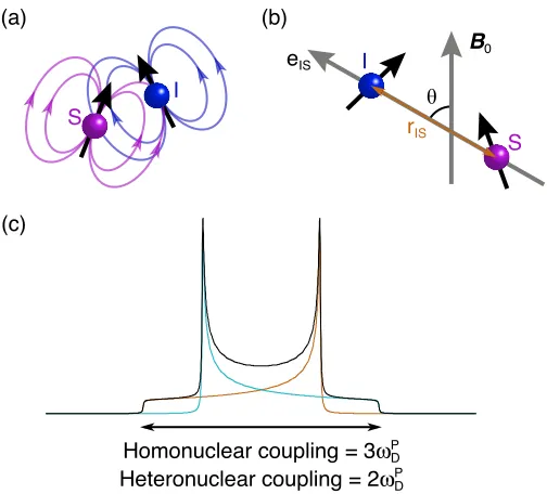
Nuclei with I ! 1/2 possess a magnetic moment or dipole, which can interact through space with other dipoles, as shown in Figure 2.5a. The resulting interaction is known as dipole-dipole coupling or more commonly, as the dipolar coupling. In the laboratory frame, the Hamiltonian is unfortunately quite complicated, as it contains many orientationally-dependent terms and therefore a simplified, truncated version of the dipolar Hamiltonian is usually used, giving

! "#

!

(a) (b)

!33

!11

!22

!iso

!xx

!zz

!yy

H_Dhomo = !

D$%3IzSz"Iz#Sz&', (2.33)

for a homonuclear dipolar coupling, and

HD

hetero _{= !}

D"#2IzSz$%, (2.34)

for a heteronuclear dipolar coupling. The dipolar splitting parameter is given by

!D = !D P 1

2 3cos

2_{" #}

1

(

)

which is dependant on the angle, !, between the internuclear vector, eIS, joining

the two dipolar coupled nuclei and the magnetic field B0, as shown in Figure 2.5b.

The dipolar coupling constant in the principal axis frame, P, is given by

!D

P ₌ µ0

4"

!#I#S

rIS

3 , (2.36)

and is dependent on the gyromagnetic ratios of the nuclei involved and the inverse

cube of the distance, rIS

3_{, between the two nuclear spins. It should also be noted}

that the dipole-coupling tensor is traceless, i.e., there is no isotropic component.

Therefore in solution, the rapid tumbling motion of the molecules effectively

removes the dipolar interaction from the spectrum.

When considering an isolated system of two spins, the dipolar coupling will

produce a splitting of 3!_DP _{for a homonuclear dipolar coupling and}

2!_DP _{for a}

hetronuclear dipolar coupling as shown in Equations 2.33 and 2.34 respectively.

However, as discussed in the previous section, in a powder sample, there will be

multiple orientations, leading to powder pattern lineshapes called “Pake

doublets”. The Pake doublet results from the overlap of two axially symmetric

anisotropicaly broadened lineshapes as shown in Figure 2.5c. In reality, however,

the classic Pake doublet lineshape is rarely found, as spins are typically affected

by numerous different dipolar couplings of different magnitudes and by different

2.2 NMR interactions

!

Figure 2.5: (a) Schematic diagram of dipole-dipole coupling, where magnetic fields of interacting

nuclear spins, I and S, are shown. (b) The distance between two dipolar coupled nuclei, rIS, is

shown along the internuclear vector, eIS, which is orientated at an angle of ! to the magnetic field

B0. (c) Powder lineshape of the I (or S) spin in a two-spin system, where the spitting is 3!D P _{for a}

homonuclear dipolar coupling and 2!D

P _{for a heteronuclear dipolar coupling.}

2.2.5 Quadrupolar coupling

Quadrupolar nuclei are those which possess a spin quantum number, I > 1/2.

The distinguishing feature of these nuclei, is the asymmetric distribution of charge

in the nucleus, described by the electric nuclear quadrupole moment, Q. This

quadrupole moment interacts with the electric field gradient tensor, V. In the

principal axis frame, V can be described by three principal components, Vxx

P_{, V}

yy

P

and Vzz

P_{. The magnitude of the interaction is defined by}

Vzz

P ₌

eq, where the

superscript P signifies the principal axis frame. It is also important to note that the

electron field gradient tensor is traceless, i.e., there is no isotropic component. The

form of the quadrupolar Hamiltonian that describes the interaction between the

nuclear electric quadrupole moment and the electric field gradient is

(b)

I

S

!

B0

eIS

(a)

I

S _r

IS

(c)

P

Homonuclear coupling = 3!D

Heteronuclear coupling = 2!D

HQ =

eQ

2I

(

)

The quadrupolar interaction is generally defined by two parameters, the

quadrupolar coupling constant, which describes the magnitude of the interaction

C_Q = eq!eQ

! =

V_zzP_! eQ

! , (2.38)

and the quadrupolar asymmetry parameter, which describes the shape of the

electric field gradient tensor,

!Q =

Vxx P_"

Vyy P

Vzz

P . (2.39)

with values between 0 and +1.

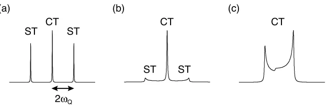
The perturbation of the Zeeman energy levels by the quadrupolar interaction to

a first-order approximation can be seen in Figure 2.6, where the single-quantum

central transition, CT,

(

)

(

)

interaction. However, the single-quantum satellite transitions, ST,

m_I = !1 / 2 " !3 / 2

(

)

(

)

transitions as shown in Figure 2.7a. The frequency of the single-quantum

transition to a first order approximation, !( )1 _{, between}

m_I = ±

(

)

where q is 1/2, 3/2, 5/2 etc, is given by

!_±( )#q"1 ±q 1

( ) _{= ±}

₍

₎

Q, (2.40)

where the quadrupole splitting parameter is

!Q =

1 2!Q

P

3cos2" #1+$Qsin 2_"

cos 2%

2.2 NMR interactions

!

Figure 2.6: Perturbation of the Zeeman energy levels for a spin I = 3/2 nucleus by the first- and second-order quadrupolar interaction. The quadrupolar broadening to the first-order approximation

results in a perturbation of the energy levels which does not affect the central single-quantum

transition and triple-quantum transitions, but does affect the two satellite transitions. The

quadrupolar broadening to the second-order approximation results in a perturbation of all energy

levels and transitions.

and the angles define the orientation of the electric field gradient tensor in the

laboratory frame. The quadrupole splitting parameter, given in rad s–1 _{in the}

principal axis frame, is

!Q

P = 3"CQ

2I

(

)

For a powdered solid, the orientational dependence of !Q results in a broadening

of the satellite transitions, while the central transition remains much sharper, as

shown in Figure 2.7b.

As the magnitude of the quadrupolar interaction increases, this first-order

perturbation will not be sufficient to fully describe the interaction and so a

second-order correction must be applied. As shown in Figure 2.6, the central

transition and triple-quantum transitions are now perturbed, resulting in a more

mI = –3/2

mI = +3/2

mI = –1/2

mI = +1/2

!0

!0

!0

!0

!0 +2!Q

!0–2!Q

Zeeman First-order quadrupolar

Figure 2.7: Static NMR spectra simulated for a I = 3/2 nucleus subject to a first-order quadrupolar

coupling for (a) a single crystal and (b) a powdered solid. In (c) the anisotropic broadening of the

CT resulting from the second-order quadrupolar interaction is shown.

anisotropic broadening of the resulting lineshapes in a powdered solid, as shown

in Figure 2.7c. The frequency of a single-quantum transition is now the sum of the

first- and second-order contributions,

!_±( )q"1#±q = !±( )q"1#±q

1

( ) _+!

±( )q"1#±q

2

( ) _{, (2.43)}

with

!_{±( )q"1#±}q 1

( ) _{= ±}

₍

₎

Q P

d0,0 2

( )

, (2.44)

!( )_±2_{( )q"1#±q =} !Q

P

( )

!0 $ % & & ' ( ) )

A0

( )

( )

2

( )

+A4

( )

4

( )

-1-, (2.45)

where the second- and fourth-rank reduced Wigner rotation matrix elements are

d0,0

2

( )

2 3cos

2_{! "}

1

(

)

d0,0

4

( )

8 35 cos 4_{! "}

30 cos2_!+ 3

(

)

and where for simplicity, axial symmetry has been assumed.25,26

ST CT ST

ST CT

ST

2!Q

(a) (b) (c)

2.3 Magic angle spinning

!

The quadrupolar interaction is typically the most dominant interaction in I >

1/2 nuclei, where, in extreme cases, the quadrupolar broadened NMR powder

patterns can be a number of MHz in breadth. This can result in extremely low

signal to noise ratios, as the total integrated signal intensity is spread out over an

extremely large spectral lineshape.

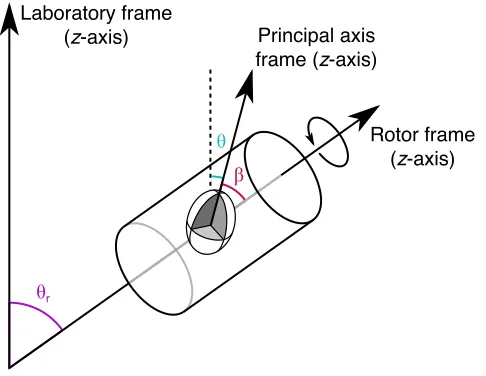
2.3 Magic angle spinning

2.3.1 Orientation dependence of interactions

Magic angle spinning, commonly abbreviated to MAS was developed by

Andrew et al.27-29 and independently by Lowe30. It is a method for mimicking the

fast molecular tumbling found in solution-state NMR which removes many of the

anisotropic interactions detailed in the previous section.31 MAS involves the rapid

rotation of a powdered sample around an axis which is inclined at an angle of

54.74° to the magnetic field B0, referred to as the “magic angle”. The rapid

rotation of the crystallites at the magic angle serves to remove or average out

specific NMR interactions that possess an orientation dependence proportional to

3cos2! "1. This includes the chemical shift anisotropy in Equation 2.32, the

dipolar coupling in Equation 2.35, the first-order quadrupolar coupling in

Equation 2.41 and part of the second-order quadrupolar coupling in Equation 2.46

(There is an additional term in Equation 2.47 which cannot be removed through

magic angle spinning).

A schematic diagram showing the implementation of MAS is shown in Figure

2.8, where a rotor is aligned and spins around an axis inclined at !r = 54.74° to

the magnetic field. As the rotor is spinning, the angle of the crystallite to the rotor

Figure 2.8: Schematic diagram showing the relevant angles between the principal axis, rotor and

laboratory frames for the purposes of MAS. The angle between the laboratory and rotor frame is

!r, the angle between the principal axis and rotor frame is ! and the angle between the principal

axis and laboratory frame is ". Under MAS !r is set to the magic angle of 54.74°, ! remains

constant and " will take on all possible values, which results in the interactions being averaged to

zero, if the rotation rate is sufficiently rapid.

field, ", will take on all possible values. Therefore, under fast MAS rates,

(typically when the MAS rate is greater than the magnitude of the interaction that

is to be removed), the anisotropy will be averaged to zero.

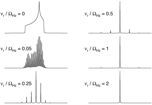
2.3.2 Effect of MAS on the CSA interaction

The effect of a variety of different MAS rates, #r, upon a CSA broadened

lineshape, where ! = 3 kHz and " = –0.5 is shown in Figure 2.9. Under static

conditions (#r/!Hz = 0), a powder pattern lineshape is observed. Under slow MAS

conditions e.g., #r/!Hz = 0.05, a large number of “spinning sidebands” appear,

which are spaced at increments of the MAS rate from the isotropic peak. The

origin of these spinning sidebands is explained in more detail in Appendix A. As Laboratory frame

(z-axis) Principal axis

frame (z-axis)

! "

"r

Rotor frame

2.3 Magic angle spinning

!

Figure 2.9: NMR spectra simulated for a spin I = 1/2 nucleus subject to CSA with ! = 3 kHz and

" = –0.5, at a variety of MAS rates, which are quoted in !r/!Hz.

MAS rate is greater than the size of the interaction e.g.,!r/!Hz = 2, the interaction

is effectively removed from the NMR spectrum and only an isotropic peak is

observed.

MAS can, therefore, be used to completely remove the CSA and similar to a

static powder pattern lineshape, the principal shielding tensor components can be

measured from a slow spinning MAS spectrum providing that that a sufficient

number of spinning sidebands are obtained.32 A more detailed description of the

number of sidebands required to accurately measure the principal tensors is given

later in Section 5.3.1.

!_r / "_Hz = 0.05

!_r / "_Hz = 0.25

!r / "Hz = 0.5

!_r / "_Hz = 1

!_r / "_Hz = 2

2.4 NMR experiments

2.4.1 Spin echo

Immediately after a rf pulse is applied to a NMR probe in a strong magnetic

field, unwanted acoustic oscillations, which are produced by the probe, generate rf

signals that are detected by the coil. Acoustic ringing is also noticeably longer at

high magnetic field strengths and when acquiring NMR spectra of nuclei with low

frequencies.33 Therefore, if the acquisition period starts immediately after the rf

pulse is turned off, these unwanted oscillations will be acquired alongside the

FID. If these unwanted oscillations overlap with a significant proportion of the

FID, significant distortions to the Fourier transformed spectrum will result.

Typically in a NMR experiment, a preacquisition delay is used after the final

pulse and before the acquisition of the FID. This time period, commonly known

as the “deadtime”, allows the unwanted acoustic ringing to die away before the

acquisition of FID, as shown in Figure 2.10a. In this thesis these intervals were

typically ~10 µs for high-! nuclei and ~100 µs for low-! nuclei. In many situations, the deadtime is only a small fraction of the length of the FID and does

not result in noticeable distortions to the FID. However, for the case of low-!

nuclei where the acoustic ringing period is longer, or static NMR spectra where

the FID length is typically much shorter, this deadtime can result in the loss of a

significant portion of the FID, leading to distortions in the Fourier transformed

spectrum. In these situations the use of a spin echo can be used to refocus the

magnetisation after the deadtime, allowing the acquisition of a complete and

undistorted FID.

The spin echo,

(

)

( )

2.4 NMR experiments

!

Figure 2.10: (a) In a conventional NMR experiment, after a !/2 pulse, acoustic ringing effects

(shown in purple) will take time to decay, overlapping with the FID (shown in blue). (b) A spin

echo pulse sequence, with !/2 pulses shown in black and ! pulses in grey. The " interval results in

a refocusing of the magnetisation at a time " enabling the acquisition of a complete FID.

pulse is applied along the x-axis, the spins will start to dephase in the transverse

plane during the time ". Through the application of a ! pulse along the y-axis, the

spins can be inverted and if left for a second period ", the magnetisation will be

refocused. Therefore, as long as the time period " is longer than the deadtime, a

complete and undistorted FID can be acquired.

2.4.2 CPMG

The spin echo experiment described in the previous section is used to acquire

what is known as a “half echo”. Carr and Purcell35 used a series of these spin

echoes in the Carr-Purcell pulse sequence,

(

)x

( )x

( )x

Through the use of additional #$! "

( )

n blocks, the magnetisation can be

continually refocused, leading to the acquisition of a series of “whole echoes”.

However, as a result of the phase of the ! pulses, the echoes are formed along the

–y and +y axes. Therefore, if there is any error in the length of the ! pulses, this

will result in a cumulative error where the magnetisation is rotated further and

further from the transverse (xy) plane. This issue was later addressed by Meiboom (b)

! !

y x

(a)

dead time x

Figure 2.11: (a) Pulse sequence for a CPMG experiment, where !/2 pulses are shown in black and

! pulses in grey. The magnetisation is refocused at a period " after each ! pulse resulting in a

series of echoes in acquisition. (b) A simulated NMR spectrum resulting from the Fourier

transformation of a half echo and a CPMG echo train.

and Gill36 who developed the Carr-Purcell-Meiboom-Gill (CPMG) pulse

sequence,

(

)

( )

( )

change in phase of the ! pulses, all of the echoes are now all formed along the +y

axis, with any errors being cancelled out following each even-numbered pulse.

The first half echo produced in a CPMG experiment is generally included in

the Fourier transformed FID so as to minimise the phasing of the spectrum

required after Fourier transformation and also to reduce baseline distortions.37 The

Fourier transformation of the series of echoes results in a series of spikelets

spaced by 1/2", which map out the intensity of the lineshape produced from a

standard Fourier transformation of a half (or single full) echo, as shown in Figure

2.11b. Therefore, the resolution of the lineshape is significantly reduced for

CPMG. However, the resulting spectrum has significantly improved peak height

sensitivity. Therefore, CPMG is best suited for the acquisition of broad lineshapes

and for nuclei where sensitivity is limited. In the case of CPMG applied under

MAS, the " interval is set to be ! = n!r to ensure coincidence of rotary and spin

echoes, i.e., synchronised with the sample rotation

(a) (b)

half echo

CPMG

! ! ! !

n

2.4 NMR experiments

!

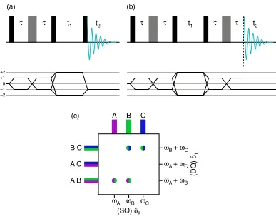
2.4.3 INADEQUATE

The incredible natural abundance double-quantum transfer experiment38,39 or

INADEQUATE, developed for solution-state NMR, is a homonuclear correlation

technique which reveals connectivities through the J-coupling, i.e., through-bond

couplings. The pulse sequence for the experiment is given in Figure 2.12a. Lesage

et al. showed that, although the INADEQUATE experiment can be carried out in

the solid state, the efficiency of the experiment was found to rapidly decrease with

increasing linewidth of the resonance owing to the resulting anti-phase

lineshapes.40 This problem can be addressed through the use of the

refocused-INADEQUATE experiment,41 shown in Figure 2.12b.

In the INADEQUATE experiment, the first !/2 pulse generates transverse

magnetisation, while the following spin echo duration creates the

antiphase-magnetisation necessary for the generation of double-quantum coherence. The

efficiency of the conversion from single-quantum (SQ) to double-quantum (DQ)

coherence is governed by the interval ", where maximum and minimum

double-quantum coherence are generated when ! = 1 / 4

( )

( )

respectively, and J is the magnitude of the isotropic J-coupling. Double-quantum

coherence can then be generated by a !/2 pulse, and it subsequently evolves

during a time, t1, (with a frequency !DQ = !SQ A _+!

SQ

B _{) for two spins A and B}

before being converted back to anti-phase magnetisation by a third !/2 pulse. In

the original solution-state experiment, the FID is acquired at this point as in

Figure 2.12a, however, in solids, particularly disordered solids, there are a range

of chemical shifts present and therefore a range of anti-phase lineshapes which

would result in unwanted cancelation of the signal. Therefore, for solids, the

efficiency of the experiment can be significantly improved by the addition of a

final refocusing step, i.e., a spin echo, which can convert the anti-phase

Figure 2.12: (a) Pulse sequence and coherence pathway diagram for the solution-state

INADEQUATE experiment, with !/2 pulses shown in black and ! pulses in grey. (b) Pulse

sequence and coherence pathway diagram for the solid-state refocused-INADEQUATE

experiment, with an additional spin echo. (c) A schematic spectrum for a

refocused-INADEQUATE experiment upon a system with three spins, A, B and C. The cross peaks show the

presence of a J-coupling between B and C, and between A and B, but not between A and C. Phase

cycling for the refocused-INADEQUATE experiment is given in Appendix B.

A schematic of a refocused-INADEQUATE NMR spectrum is shown in Figure

2.12c where the resonances in the indirect, or double-quantum dimension are at

frequencies given by the sum of the two J-coupled resonances in the direct, or

single-quantum dimension. These cross peaks show that there is a J-coupling

between spins B and C, and between A and B, but not between A and C. (c)

(a)

(SQ) !₂

(DQ)

!1

"_A + "_C

A B C

"_A + "_B "_B + "_C

"_B "_C "_A

B C

A C

A B

(b)

# # t₁ t₂ # # t₁ # # t₂

2.5 Computational chemistry !

2.5 Computational chemistry

2.5.1 Introduction

Solid-state NMR spectra are in many cases quite complex and difficult to

interpret, owing to the multitude of interactions that can affect them.

First-principles calculations are now increasingly popular, due to their proven ability to

help interpret, assign and predict NMR spectra and hence, to provide a link

between experiment and structural information. The use of computational

chemistry in this thesis is confined to the use of a single program. The Cambridge

Serial Total Energy Package (CASTEP)42,43 code exploits the inherent periodicity

of inorganic solids and calculates the NMR parameters of all nuclei in the system,

which can then be utilised to aid the interpretation of solid-state NMR spectra.

CASTEP is a first-principles approach, using density-functional theory, DFT.

2.5.2 The Schrödinger equation

The non-relativistic time-independent Schrödinger equation contains all the

information required to calculate the energies and, therefore, the properties, (such

as the NMR parameters) of a system, and is given by

ˆ

H!

(

)

(

)

where _Hˆ _{is the Hamiltonian operator for a system which contains M nuclei and N}

electrons, E is the total energy and ! is the wavefunction of the system, described

by the 3N spatial coordinates (ri)and the N spin coordinates (si) of the electrons,

collectively termed (xi) and the 3M spatial coordinates (Ri) of the nuclei. The

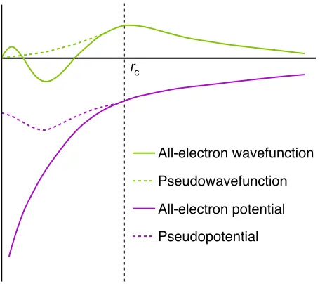
Schrödinger equation can be simplified through the use of the Born-Oppenheimer

comparison to electrons, therefore, the system can be thought of as comprising of

fixed nuclei and moving electrons. Therefore, we can remove the spatial

coordinates of the nuclei to produce the so-called electronic Hamiltonian,

ˆ

H_elec!_elec

(

)

(

)

It can be seen that the description of the wavefunction has been considerably

simplified, as it now requires only 4N instead of 4N and 3M variables. However,

owing to the number of electrons in even a modest sized molecular system, this is

still generally impossible to solve, and so a different approach is required.

2.5.3 Density functional theory

A radically different approach to the calculation of the energies of a system

was introduced by Hohenberg and Kohn,45 with the methodology later developed

by Kohn and Sham,45 in which it was realised that the complicated N-electron

wavefunction can be replaced by the electron density, !

( )

dependant on at most two particles at a time, independent of the size of the

system. We can therefore describe the complete ground state energy as a

functional of the ground state electron density,

E

[ ]

[ ]

[ ]

[ ]

[ ]

where TS is the exact kinetic energy of a system of non-interacting electrons

which produces the true ground state electron density, Vext is the external potential

energy (the interaction of the electrons with the fixed atomic nuclei) and VH is the

Hartree energy. The final term, EXC, is the exchange correlation energy which is

not known and must be approximated.

2.5 Computational chemistry !

proposed that EXC can be described by the exchange correlation energy per

particle of a uniform electron gas of similar density !XC, leading to the local

density approximation (LDA)

EXC

LDA

[ ]

r

( )

"

( )

( )

Despite working quite well in some cases, the LDA approach is not always the

best solution as it neglects to include any information about the non-homogeneity

of the true electron density. The generalised gradient approximation (GGA)47-49

approach includes an additional term that incorporates some dependence on the

gradient of the charge density, which can result in improvements to the

calculation of the energy

EXC

GGA

[ ]

r

( )

"

(

( )

)

There are numerous proposed GGA methods, each with different

improvements. One method by Perdew, Burke and Ernzerhof (PBE)50 has been

adopted as the method of choice for use with CASTEP and widely used in the

existing literature.

2.5.4 Wavefunctions in a periodic system

Any calculation involving a crystal structure which is infinitely repeating will

clearly require some form of simplification, as it is fundamentally impossible to

consider an infinite number of particles. A rudimentary approach to approximate

this situation is to simply create a cluster of atoms of significant size, so the

central atoms “feel” as if they are in an infinitely repeating structure. However, to

achieve a sufficiently accurate representation of the structure requires a large

number of atoms. Therefore, a more elegant method would be to use only the unit

be arranged in a periodic fashion, and therefore the potential acting on the

electrons will also be periodic. Bloch’s theorem states that as the potential is

periodic, so is the density and magnitude of the wavefunction. The wavefunction

can be described as

!

( )

u_k

( )

where eikr _{is an arbitrary phase factor, u}

k

( )

point in the reciprocal space, referred to as a k-point. The periodic magnitude of

the wavefunction, uk

( )

uk

( )

G

!

in turn constructed through an infinite combination of complex Fourier

coefficients, cGk and planewaves, e

iGr

.51 There are an infinite number of

reciprocal lattice vectors, G, and therefore an infinite number of coefficients and

planewaves. However, the higher energy planewaves have a correspondingly

small coefficient and therefore contribute negligibly to the formation of the

wavefunction. It is therefore possible to restrict the number of planewaves used by

defining an energy cut-off to reduce the computational cost.

1

2G

2

< Ecut. (2.55)

Now that the wavefunctions can be constructed, in principle to construct the

electron density it would be necessary to integrate over an infinite number of k

-points. However, as the wavefunctions change slowly as k is varied, an infinite

number is not always required. Instead, this can simply be approximated by the

summation of a suitable number of k-points,

!

( )

( )

2

d3k

#

$ "k

( )

2

k