An efficient clustering algorithm for class based language models

An Efficient Clustering Algorithm for Class-based Language Models

Takuya Matsuzaki

Yusuke Miyao

Department of Computer Science, University of Tokyo

Hongo 7-3-1, Bunkyo-ku, Tokyo 113-0033 JAPAN

CREST, JST (Japan Science and Technology Corporation)

Honcho 4-1-8, Kawaguchi-shi, Saitama 332-0012 JAPAN

matuzaki,yusuke,tsujii

@is.s.u-tokyo.ac.jp

Jun’ichi Tsujii

Abstract

This paper defines a general form for class-based probabilistic language models and pro-poses an efficient algorithm for clustering based on this. Our evaluation experiments re-vealed that our method decreased computation time drastically, while retaining accuracy.

1

Introduction

Clustering algorithms have been extensively studied in the research area of natural language processing because many researchers have proved that “classes” obtained by clustering can improve the performance of various NLP tasks. Examples have been class-based-gram models

(Brown et al., 1992; Kneser and Ney, 1993), smooth-ing techniques for structural disambiguation (Li and Abe, 1998) and word sense disambiguation (Sh¨utze, 1998).

In this paper, we define a general form for class-based probabilistic language models, and propose an efficient and model-theoretic algorithm for clustering based on this. The algorithm involves three operations, CLAS-SIFY, MERGE, and SPLIT, all of which decreases the optimization function based on the MDL principle (Ris-sanen, 1984), and can efficiently find a point near the lo-cal optimum. The algorithm is applicable to more general tasks than existing studies (Li and Abe, 1998; Berkhin and Becher, 2002), and computational costs are signifi-cantly small, which allows its application to very large corpora.

Clustering algorithms may be classified into three types. The first is a type that uses various heuristic mea-sure of similarity between the elements to be clustered and has no interpretation as a probability model (Widdow, 2002). The resulting clusters from this type of method are not guaranteed to work effectively as a component of a statistical language model, because the similarity used in clustering is not derived from the criterion in the

learning process of the statistical model, e.g. likelihood. The second type has clear interpretation as a probability model, but no criteria to determine the number of clusters (Brown et al., 1992; Kneser and Ney, 1993). The perfor-mance of methods of this type depend on the number of clusters that must be specified before the clustering pro-cess. It may prove rather troublesome to determine the proper number of clusters in this type of method. The third has interpretation as a probability model and uses some statistically motivated model selection criteria to determine the proper number of clusters. This type has a clear advantage compared to the second. AutoClass (Cheeseman and Stutz, 1996), the Bayesian model merg-ing method (Stolcke and Omohundro, 1996) and Li’s method (Li, 2002) are examples of this type. AutoClass and the Bayesian model merging are based on soft tering models and Li’s method is based on a hard clus-tering model. In general, computational costs for hard clustering models are lower than that for soft clustering models. However, the time complexity of Li’s method is of cubic order in the size of the vocabulary. Therefore, it is not practical to apply it to large corpora.

Our model and clustering algorithm provide a solution to these problems with existing clustering algorithms. Since the model has clear interpretation as a probability model, the clustering algorithm uses MDL as clustering criteria and using a combination of top-down clustering, bottom-up clustering, and a K-means style exchange al-gorithm, the method we propose can perform the cluster-ing efficiently.

Sec-tions 2 and 3, that the proposed method can be applied to a broader range of tasks than the test task we evalu-ate in the experiments in Section 4. We need further ex-periments to determine the performance of the proposed method with more general tasks.

2

Probability model

2.1 Class-based language modeling

Our probability model is a class-based model and it is an extension of the model proposed by Li and Abe (1998). We extend their two-dimensional class model to a multi-dimensional class model, i.e., we incorporate an arbitrary number of random variables in our model.

Although our probability model and learning algorithm are general and not restricted to particular domains, we mainly intend to use them in natural language process-ing tasks where large amounts of lexical knowledge are required. When we incorporate lexical information into a model, we inevitably face the data-sparseness problem. The idea of ‘word class’ (Brown et al., 1992) gives a gen-eral solution to this problem. A word class is a group of words which performs similarly in some linguistic phenomena. Part-of-speech are well-known examples of such classes. Incorporating word classes into linguistic models yields good smoothing or, hopefully, meaningful generalization from given samples.

2.2 Model definition

Let us introduce some notations to define our model. In our model, we have consideredkinds of discrete

ran-dom variables

and their joint

distribu-tion.

denotes a set of possible values for the

-th

vari-able

. Our probability model assumes disjunctive

par-titions of each

, which are denoted by

’s. A

disjunc-tive partition

ofis a subset of

, and satisfies

and

.

We call elements in a partition

classes of elements in

.

, or

for short, denotes a class in

which

contains an element .

With these notations, our probability model is ex-pressed as:

½

¾

(1)

In this paper, we have considered a hard clustering model, i.e., for any . Li & Abe’s model

(1998) is an instance of this joint probability model, where. Using more than 2 variables the model can

represent the probability for the co-occurrence of triplets, such assubject, verb, object.

2.3 Clustering criterion

To determine the proper number of classes in each par-tition

, we need criteria other than the

maxi-mum likelihood criterion, because likelihood always be-come greater when we use smaller classes. We can see this class number decision problem as a model selection problem and apply some statistically motivated model selection criteria. As mentioned previously (following Li and Abe (1998)) we used the MDL principle as our clustering criterion.

Assume that we have samples of co-occurrence

data:

Ü

The objective function in both clustering and parame-ter estimations in our method is the description length,

, which is defined as follows:

(2)

wheredenotes the model and

is the likelihood

of samplesunder model:

(3)

The first term in Eq.2,

, is called the data

description length. The second term,, is called the

model description length, and when sample size is

large, it can be approximated as

where is the number of free parameters in model.

We used this approximated form throughout this paper. Given the number of classes,

for each , we have

free parameters for joint

probabilities

. Also, for each class, we

havefree parameters for conditional probabilities , where. Thus, we have

Our learning algorithm tries to minimizeby

adjusting the parameters in the model, selecting partition

of each

, and choosing the numbers of classes,

3

Clustering algorithm

Our clustering algorithm is a combination of three ba-sic operations: CLASSIFY, SPLIT and MERGE. We it-eratively invoke these until a terminate condition is met. Briefly, these three work as follows. The CLASSIFY takes a partition inas input and improves the

par-tition by moving the elements infrom one class to

an-other. This operation is similar to one iteration in the K-means algorithm. The MERGE takes a partition as

in-put and successively chooses two classes and

from and replaces them with their union,

. The SPLIT

takes a class, , and tries to find the best division of

into two new classes, which will decrease the description length the most.

All of these three basic operations decrease the de-scription length. Consequently, our overall algorithm also decreases the description length monotonically and stops when all three operations cause no decrease in de-scription length. Strictly, this termination does not guar-antee the resulting partitions to be even locally opti-mal, because SPLIT operations do not perform exhaus-tive searches in all possible divisions of a class. Doing such an exhaustive search is almost impossible for a class of modest size, because the time complexity of such an exhaustive search is of exponential order to the size of the class. However, by properly selecting the number of tri-als in SPLIT, we can expect the results to approach some local optimum.

It is clear that the way the three operations are com-bined affects the performance of the resulting class-based model and the computation time required in learning. In this paper, we basically take a top-down, divisive strat-egy, but at each stage of division we do CLASSIFY op-erations on the set of classes at each stage. When we cannot divide any classes and CLASSIFY cannot move any elements, we invoke MERGE to merge classes that are too finely divided. This top-down strategy can drasti-cally decrease the amount of computation time compared to the bottom-up approaches used by Brown et al. (1992) and Li and Abe (1998).

The following is the precise algorithm for our main procedure:

Algorithm 1 MAIN PROCEDURE()

INPUT

: an integer specifying the number of trials in a

SPLIT operation

OUTPUT

Partitions

and estimated parameters in the

model

PROCEDURE

Step 0

INITIALIZE

Step 1 Do Step 2 through Step 3 until no change is made

through one iteration

Step 2 For, do Step 2.1 through Step 2.2

Step 2.1 Do Step 2.1.1 until no change occurs through it

Step 2.1.1 For,

CLASSIFY

Step 2.2 For each ,

SPLIT

Step 3 For,

MERGE

Step 4 Return the resulting partitions with the

parame-ters in the model

In the Step 0 of the algorithm, INITIALIZE creates the initial partitions of

. It first divides each

into two classes and then applies CLASSIFY

to each partition

one by one, while any

ele-ments can move.

The following subsections explain the algorithm for the three basic operations in detail and show that they decreasemonotonically.

3.1 Iterative classification

In this subsection, we explain a way of finding a local optimum in the possible classification of elements in

,

given the numbers of classes in partitions .

Given the number of classes, optimization in terms of the description length (Eq.2) is just the same as optimiz-ing the likelihood (Eq.3). We used a greedy algorithm which monotonically increases the likelihood while updating classification. Our method is a generalized version of the previously reported K-means/EM-algorithm-style, iterative-classification methods in Kneser and Ney (1993), Berkhin and Becher (2002) and Dhillon et al. (2002). We demonstrate that the method is applicable to more generic situations than those previ-ously reported, where the number of random variables is arbitrary.

To explain the algorithm more fully, we define ‘counter functions’as follows:

ÜÜ

ÜÜ

ÜÜ

Ü

ÜÜ

Ü

where the hatch () denotes the cardinality of a set and Ü

is the

-th variable in sampleÜ. We used ,

Our classification method is variable-wise. That is, to classify elements in each

, we classified the

elements in each

in order. The precise algorithm is as

follows:

Algorithm 2 CLASSIFY( )

INPUT

: a partition in

OUTPUT An improved partition in

PROCEDURE

Step 1 Do steps 2.1 through 2.3 until no elements in

can move from their current class to another one.

Step 2.1 For each element

, choose a class

which satisfies the following two conditions:

1.

is not empty , and 2.

maximizes following quantity

:

When the class containingnow,

, maximizes , select as

even if some other classes also max-imize.

Step 2.2 Update partition

by moving each

to

the classes which were selected as

forin Step

2.1.

Step 2.3 Update the parameters by maximum likelihood

estimation according to the updated partition.

Step 3 Return improved partition .

In Step 2.3, the maximum likelihood estimation of the parameters are given as follows:

(4) To see why this algorithm monotonically increases the likelihood (Eq.3), it is sufficient to check that, for vari-able

and any classification before Steps 2 and 3,

do-ing Steps 2 and 3 positively changes the log likelihood (Eq.3). We can show this as follows.

First, assume without loss of generality. Let ½ and ½ denote

the partitions before/after Step 2, respectively. Let and

denote the classes where an element

belongs, before and after Step 2, respectively.

Also, let

denote the class which was chosen for in Step 2.1 in the algorithm. Note that

is different

from

as a set. However, with these notations, it holds

that if , then

. We also use the suffixes

in notations and

as it holds that, if , then .

Using Eq.4, we can write the change in the log likeli-hood, as follows:

½ ½ (5)

To see the difference is, we insert the intermediate

terms into the right of Eq.5 and transform it as:

½ ½ ½ ½ ½ (6) ½ (7)

In the last expression, each term in the summation (7) is according to the conditions in Step 2 of the

al-gorithm. Then, the summation (7) as a whole is always

and only equals 0 if no elements are moved. We

can confirm that the summation (6) is positive, through an optimization problem:

maximize the following quantity

½

under the condition:

for any

.

isbecause

, and

is always. Thus, the solution to this problem is given

by:

for any

. Through this, we can conclude

that the summation (6) is. Therefore,

holds, i.e., CLASSIFY increases log likelihood monoton-ically.

3.2 SPLIT operation

The SPLIT takes a class as input and tries to find a way to divide it into two sub-classes in such a way as to re-duce description length. As mentioned earlier, to find the best division in a class requires computation time that is exponential to the size of the class. We will first use a brute-force approach here. Let us simply try random

divisions, rearrange them with CLASSIFY and use the best one. If the best division does not reduce the descrip-tion length, we will not change the class at all. It may possible to use a more sophisticated initialization scheme, but this simple method yielded satisfactory results in our experiment.

The following is the precise algorithm for SPLIT:

Algorithm 3 SPLIT(,)

INPUT

: a class to be split

: an integer specifying the number of trials

OUTPUT

Two new classes and

on success, or with

no modifications on failure

PROCEDURE

Step 1 Do Steps 2.1 through 2.3 J times

Step 2.1 Randomly divideinto two classes

Step 2.2 Apply CLASSIFY to these two classes

Step 2.3 Record the resulting two classes in Step 2.2 with

the reduced description length produced by this split

Step 3 Find the maximum reduction in the records

Step 4 If this maximum reduction, return the

corre-sponding two classes as output, or return if the

maximum

Clearly, this operation decreases on success

and does not change it on failure.

3.3 MERGE operation

The MERGE takes partition as input and successively

chooses two classes and

from

and replaces them

with their union

. This operation thus reduces the

number of classes inand accordingly reduces the

num-ber of parameters in the model. Therefore, if we properly choose the ‘redundant’ classes in a partition, this merging reduces the description length by the greater reduction in the model description length which surpasses the loss in log-likelihood.

Our MERGE is almost the same procedure as that de-scribed by Li (2002). We first compute the reduction in description length for all possible merges and record the amount of reduction in a table. We then do the merges in order of reduction, while updating the table.

The following is the precise algorithm for MERGE. In the pseudo code,Æ

denotes the reduction in

which results in the merging of and

.

Algorithm 4 MERGE()

INPUT : a partition in

OUTPUT An improved partition inon success, or the

same partition as the input on failure

PROCEDURE

Step 1 For each pair

in compute Æ and

store them in a table.

Step 2 Do Step 3.1 through 3.5 until the termination

con-dition in 3.2 is met

Step 3.1 Find the maximum,Æ , in allÆ

Step 3.2 IfÆ , return the updated partition, or

else go to Step 3.3.

Step 3.3 Replace the class pair

which

corre-sponds toÆ , with their union

.

Step 3.4 Delete all Æ

’s which concern the merged

classes or

from the table.

Step 3.5 For each in

, computeÆ and

store them in the table.

It is clear from the termination condition in Step 3.2 that this operation reduceson success but does

not change it on failure.

4

Evaluation

4.1 Evaluation task

We used a simplified version of the dependency analysis task for Japanese for the evaluation experiment.

In Japanese, a sentence can be thought of as an array of phrasal units called ‘bunsetsu’ and the dependency struc-ture of a sentence can be represented by the relationships between these bunsetsus. A bunsetsu consists of one or more content words and zero or more function words that follow these.

For example, the Japanese sentence

Ryoushi-ga kawa-de oyogu nezumi-wo utta. hunter-SUBJ river-in swim mouse-OBJ shot

(A hunter shot a mouse which swam in the river.)

contains five bunsetsus Ryoushi-ga, kawa-de, oyogu,

nezumi-wo, uttaand their dependency relations are as

follows:

Ryoushi-gautta kawa-deoyogu

oyogunezumi-wo nezumi-woutta

Our task is, given an input bunsetsu, to output the cor-rect bunsetsu on which the input bunsetsu depends. In this task, we considered the dependency relations of lim-ited types. That is the dependency of types: noun-pp

pred , where noun is a noun, or the head of a compound

noun, pp is one of 9 postpositionsga, wo, ni, de, to,

he, made, kara, yoriand pred is a bunsetsu which

con-tains a verb or an adjective as its content word part. We restricted possible dependee bunsetsus to be those to the right of the input bunsetsus because in Japanese, basically all dependency relations are from left to right. Thus, our test data is in the form

noun-pppred

pred

(8)

wherepred

,...,pred

is the set of all candidate

de-pendee bunsetsus that are to the right of the input depen-dent bunsetsu noun-pp in a sentence. The task is to select the correct dependee of noun-pp frompred

,..,pred .

Our training data is in the form, noun, pp, pred.

A sample of this form represents two bunsetsus,

noun-pp and pred within a sentence, in this order, and denotes whether they are in a dependency relation

( ), or not ( ). From these types of samples,

we want to estimate probabilitynounpppredand

use these to approximate probability

, where given the

test data in Eq.8, predis the correct answer, expressed

as

nounpppred

nounpppred

We approximated the probability of occurrence for sample typeexpressed as

nounppprednounpppred

and estimated these from the raw frequencies. For the probability of type , we treated a pair of pp and

pred as one variable, pp:pred, expressed as

nounpppred

nounpp:pred

and estimated

nounpp:predfrom the training data.

Thus, our decision rule given test data (Eq.8) is, to select pred where

is the index which maximizes the

value

nounpp:pred

pppred

We extracted the training samples and the test data from the EDR Japanese corpus (EDR, 1994). We ex-tracted all the positive (i.e.,) and negative ()

relation samples and divided them into 10 disjunctive sets for 10-fold cross validation. When we divided the sam-ples, all the relations extracted from one sentence were put together in one of 10 sets. When a set was used as the test data, these relations from one sentence were used as the test data of the form (Eq.8). Of course, we did not use samples with only one pred. In the results in the next subsection, the ‘training data of size’ means where we

used a subset of positive samples that were covered by the most frequentnouns and the most frequentpp:pred

pairs.

4.2 Results

In this experiments, we compared three methods: ours, Li’s described in Li (2002), and a restricted version of our method that only uses CLASSIFY operations. The last method is simply called ‘the CLASSIFY method’ in this subsection. We used 10 as parameter in our

method, which specifies the number of trials in initializa-tion and each SPLIT operainitializa-tion. Li’s method (2002) uses the MDL principle as clustering criteria and creates word classes in a bottom-up fashion. Parameters and in

his method, which specify the maximum numbers of suc-cessive merges in each dimension, were both set to 100. The CLASSIFY method performs K-means style itera-tive clustering and requires that the number of clusters be specified beforehand. We set these to be the same as the number of clusters created by our method in each train-ing set. By evaluattrain-ing the differences in the performance of ours and the CLASSIFY method, we can see advan-tages in our top-down approach guided by the MDL prin-ciple, compared to the K-means style approach that uses a fixed number of clusters.We expect that these advantages will remain when compared to other previously reported, K-means style methods (Kneser and Ney, 1993; Berkhin and Becher, 2002; Dhillon et al., 2002).

In the results, precision refers to the ratio!!"

and coverage refers to the ratio!#, where!and"denote

the numbers of correct and wrong predictions, and#

1 10 100 1000 10000 100000

1000 10000 100000

computation time (sec)

size of vocabulary

our method Li’s method CLASSIFY

Figure 1: Computation time

10 100 1000 10000 100000

0 0.05 0.1 0.15 0.2 0.25 0.3 0.35 0.4 0.45

computation time(sec)

coverage

our method Li’s method

Figure 2: Coverage-Cost plot

treated as wrong answers ("), where a ‘tie case’ means

a situation where two or more predictions are made with the same maximum probabilities.

All digits are averages of results for ten training-test pairs, except for Li’s method where the training sets were 8k or more. The results of the Li’s method on training set of 8k were the averages over two training-test pairs. We could not do more trials with Li’s method due to time constraints. All experiments were done on Pentium III 1.2-GHz computers and the reported computation times are wall-clock times.

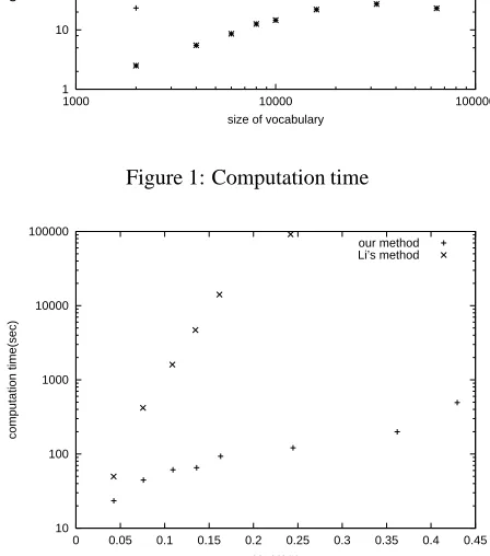
Figure 1 shows the computation time as a function of the size of the vocabulary, i.e., the number of nouns plus the number of case frame slots (i.e., pp:pred) in the train-ing data. We can clearly see the efficiency of our method in the plot, compared to Li’s method. The log-log plot re-veals our time complexity is roughly linear to the size of the vocabulary in these data sets. This is about two orders lower than that for Li’s method.

There is little relevance in comparing the speed of the

0.74 0.75 0.76 0.77 0.78 0.79 0.8 0.81

0 0.05 0.1 0.15 0.2 0.25 0.3 0.35 0.4 0.45

precision

coverage

our method Li’s method CLASSIFY

Figure 3: Coverage-precision plot

CLASSIFY method to the speed of the other two meth-ods, because its computation time does not include the time required to decide the proper number of classes. Of more interest is to see its seeming speed-up in the largest data sets. This implies that, in large and sparse training data, the CLASSIFY method was caught in some bad lo-cal optima at some early points on the way to better lolo-cal optima.

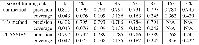
Figure 2 has the computation times as a function of the coverage which is achieved using that computation time. From this, we would expect our method to reach higher coverage within a realistic time if we used larger quantities of training data. To determine this, we need other experiments using larger corpora, which we intend to do in the future.

Table 1 lists the description lengths for training data from 1 to 32k and Table 2 shows the precision and cov-erage achieved by each method with this data. In these tables, we can see that our method works slightly better than Li’s method as an optimization method which min-imizes the description length, and also in the evaluation tasks. Therefore, we can say that our method decreased computational costs without losing accuracy. We can also see that ours always performs better than the CLASSIFY method. Both ours and the CLASSIFY method use ran-dom initializations, but from the results, it seems that our top-down, divisive strategy in combination with K-means like swapping and merging operations avoids the poor lo-cal optima where the CLASSIFY method was caught.

Figure 3 also presents the results in terms of coverage-precision trade-off. We can see that our method selected always better points in the trade-off than Li’s method or the CLASSIFY method.

ap-size of test data 1k 2k 3k 4k 5k 8k 16k 32k our method 1.15 1.88 2.38 2.76 3.13 3.77 5.03 6.21 Li’s method 1.16 1.89 2.40 2.80 3.17 3.85 N/A N/A CLASSIFY 1.16 1.89 2.39 2.77 3.14 3.79 5.08 6.31

Table 1: Description length in training data sets (unit:

)

size of training data 1k 2k 3k 4k 5k 8k 16k 32k our method precision 0.805 0.799 0.798 0.794 0.791 0.797 0.780 0.745

coverage 0.043 0.076 0.109 0.136 0.163 0.245 0.362 0.429 Li’s method precision 0.802 0.795 0.793 0.786 0.784 0.791 N/A N/A

coverage 0.043 0.076 0.109 0.135 0.162 0.242 N/A N/A CLASSIFY precision 0.797 0.792 0.789 0.785 0.786 0.789 0.768 0.741

coverage 0.042 0.075 0.108 0.135 0.162 0.242 0.356 0.427

Table 2: Performance of each method in the evaluation task

proach with the MDL principle will have advantages in large and sparse data compared to existing K-means style approaches where the number of the clusters is fixed.

5

Conclusion

This paper proposed a general, class-based probability model and described a clustering algorithm for it, which we evaluated through experiments on a disambiguation task of Japanese dependency analysis. We obtained the following results. (1) Our clustering algorithm was much more efficient than the existing method that uses the same objective function and the same kind of model. (2) It worked better as an optimization algorithm for the de-scription length than the existing method. (3) It per-formed better in the test task than an existing method and another method that is similar to other existing methods.

References

Andreas Stolcke and Stephen M. Omohundro. 1994. Best-first Model Merging for Hidden Markov Model Induction. Technical Report TR-94-003, Computer Science Division, University of California at Berkeley and International Science Institute.

Dominic Widdow and Beate Dorow. 2002. A Graph Model for Unsupervised Lexical Acquisition. Pro-ceedings of the 19th International Conference on Com-putational Linguistics, 1093–1099.

EDR. 1994. EDR (Japanese Electronic Dictionary Re-search Institute, Ltd) dictionary version 1.5 technical guide.

Hang Li. 2002. Word Clustering and Disambiguation based on Co-occurrence Data, Natural Language

En-gineering, 8(1), 25-42.

Hang Li and Naoki Abe. 1998. Word Clustering and Disambiguation Based on Co-occurrence data.

Pro-ceedings of the 18th International Conference on Com-putational Linguistics and the 36th Annual Meeting of Association for Computational Linguistics, 749–755.

Hinrich Sch¨utze. 1998. Automatic Word Sense Discrim-ination Computational Linguistics, 24(1) 97–124.

Inderjit S. Dhillon, Subramanyam Mallela and Rahul Ku-mar. 2002. Information Theoretic Feature Clustering for Text Classification. The Nineteenth International

Conference on Machine Learning, Workshop on Text Learning.

Jorma Rissanen. 1984. Universal Coding, Information, Prediction, and Estimation. IEEE Transactions on

In-formation theory, Vol. IT-30(4):629–636

Pavel Berkhin and Jonathan Becher. 2002. Learning Simple Relations: Theory and Applications. In

Pro-ceedings of the Second SIAM International Conference on Data Mining, 420–436.

Peter F. Brown, Vincent J. Della Pietra, Peter V. deSouza, Jennifer C. Lai and Robert L. Mercer. 1992. Class-Based n-gram Models of Natural Language.

Compu-tational Linguistics 18(4):467-479.

Peter Cheeseman and John Stutz. 1996. Bayesian Clas-sification (AutoClass): Theory and Results. In U. Fayyad, G. Piatetsky-Shapiro, P. Smyth and R. Uthu-rusamy (Eds.), Advances in Knowledge Discovery and

Data Mining, 153–180. AAAI Press.

Reinherd Kneser and Hermann Ney. 1993. Improved Clustering Techniques for Class-Based Statistical Lan-guage Modelling. In Proceedings of the 3rd European