Power Quality Data Compression Based on Iterative PCA Algorithm in Smart Distribution Systems

ISSN Online: 2151-4844 ISSN Print: 2151-481X

DOI: 10.4236/sgre.2017.812024 Dec. 21, 2017 366 Smart Grid and Renewable Energy

Power Quality Data Compression Based on

Iterative PCA Algorithm in Smart Distribution

Systems

Ming Zhang

1*

, Yiming Zhan

1

, Shunfan He

2

1_{School of Electronic and Electrical Engineering, Wuhan Textile University, Wuhan, China}

2_{College of Computer Science, South Central University for Nationalities, Wuhan, China}

Abstract

To reduce the stress of data transmission and storage for power quality (PQ) in smart distribution systems and help PQ analysis, a multichannel data com-pression based on iterative PCA (principal component analysis) algorithm is introduced. The proposed method uses PCA to reduce the redundancy of data to achieve the purpose of compressing data. In order to improve the calculat-ing speed, an iterative method is proposed to compute the principal compo-nents of the covariance matrix. The correctness and feasibility of the proposed method are verified by field PQ data tests. Compared with discrete wavelet transform (DWT) method, the proposed method has good performance on compression ratio and reconstruction accuracy.

Keywords

Smart Distribution Systems, Power Quality, Data Compression, Principal Component Analysis (PCA)

1. Introduction

As the growing demand for smart distribution systems, more and more power quality (PQ) monitors are especially needed for the power systems with distri-buted power sources and impulsive and sensitive loads [1][2][3]. In power sys-tems, short circuit fault, capacitor switching device for power factor compensa-tion, power electronic device for special loads etc. bring various PQ disturbances (PQD). With the deployment of a large number of PQ monitors, a big volume of data will be produced for smart distribution systems. And it becomes essential to compress this volume so that the data sets can be transmitted and stored

How to cite this paper: Zhang, M., Zhan, Y.M. and He, S.F. (2017) Power Quality Data Compression Based on Iterative PCA Algorithm in Smart Distribution Systems. Smart Grid and Renewable Energy, 8, 366-378.

https://doi.org/10.4236/sgre.2017.812024 Received: November 16, 2017

Accepted: December 19, 2017 Published: December 22, 2017 Copyright © 2017 by authors and Scientific Research Publishing Inc. This work is licensed under the Creative Commons Attribution International License (CC BY 4.0).

http://creativecommons.org/licenses/by/4.0/

DOI: 10.4236/sgre.2017.812024 367 Smart Grid and Renewable Energy promptly and efficiently. Hence, PQ data compression calls more concerns than ever before [4].

The main goal of any compression method is to achieve maximum data re-duction and preserving morphology features upon reconstruction. Data com-pression is categorized into methods on lossless and lossy techniques. Lossless methods can obtain an exact reconstruction of the original signal, but high compression ratio (CR) cannot be obtained. In contrast, lossy methods do not obtain an exacter construction, but higher CR can be achieved. Consequently, the commonly used PQ data compression methods are lossy in nature [5][6].

In general, the data compression scheme for PQ data consists of three steps: signal transform, quantization and encoding. With respect to quantization and encoding, the researchers are more concerned with signal transform. Literature

[7] firstly started the PQD data compression by wavelet transform (WT). A threshold was set to eliminate small wavelet coefficients. Improved wave-let-based methods with different threshold settings were also used in this field

[8][9][10]. Currently a popular PQD data compression is the quantization me-thod [11] [12]. These methods separate fundamental component and distur-bance components in power signals. The fundamental component and harmonic components are compressed in the data form of amplitude, frequency and phase angle by Fourier transform (FT). While other PQD components, if there are, are compressed by WT. The key of the quantization methods is how to distinguish the PQD components and separate them with little distortion to fundamental and harmonic components. Since periodical PQ signal is compressed by FT, and the signal compressed by WT is with much less low frequency components, the quantization methods have much higher CR than traditional methods. Another interesting PQ data compression method is developed based on singular value decomposition (SVD) [13]. The PQ data is transformed into singular value ma-trix that contains nonzero singular values by SVD so that the data can be com-pressed. The method is also exploring different takeoffs between data CR and loss of information. However, the SVD algorithm is easily affected by the out-liers and noises in the data.

gen-DOI: 10.4236/sgre.2017.812024 368 Smart Grid and Renewable Energy erally large, the time-consuming of the traditional PCA is very large. In order to improve the calculating speed, an iterative method is proposed to compute the principal components of the covariance matrix.

The remainder of this paper is organized as follows. The PCA algorithm is in-troduced in Part 2; Part 3 presents the proposed method; Part 4 provides field PQ data to test and compare the proposed method with related works; Part 5 summarizes the whole work.

2. PCA Algorithm

PCA algorithm was invented in 1901 by Karl Pearson, and it uses an orthogonal transformation to convert a set of measurements of possibly correlated variables into a set of values of linearly uncorrelated variables called principal compo-nents. The main advantage of PCA can reduce the dimension and redundancy of data. The eigenvalues and eigenvectors are obtained by decomposing the cova-riance matrix of data. Then the eigenvectors corresponding to several larger ei-genvalues are found as the principal components, and the projection of the measured data to the principal components is carried out to represent the origi-nal data, so as to achieve the reduction of dimension and redundancy of data.

Suppose that a sample set X contains m samples, and the dimension of each sample is n: X =

{

x x1, 2,,xm

}

,

(

1, 2, ,

)

n

i i i in

x = x x  x ∈R .

Representing each sample as a row, the m n× sample matrix S is the stack of all such rows, and m n

R ×

∈

S , then the samples are processed by zero mean, that is, the samples are centralized, to ensure that the average value of each dimen-sion of the matrix is zero.

1

1 m i i

x x

m =

=

∑

(1)

i i

x = −x x

 (2) The sample matrix composed of xi is denoted as S, where

m n

R ×

∈

S , then the covariance matrix C of S is obtained as follows:

T T

1 1

i

m

i i

x x

m m

= =

∑

C S S    (3)

where C is a real symmetric matrix, and C∈Rn n× . T

i

x

 and T

S are the transpose of xi and S, respectively. According to the matrix theory, a real

symmetric matrix can be diagonalized, therefore there is an orthogonal matrix P

that meets T =

P CP Λ. The following process is applied to obtain the matrix P. Firstly the matrix C is decomposed to get the diagonal matrix Λ and the or-thogonal matrix P. Obviously, P,Λ∈Rn n× . Then a new diagonal matrix Λ1 is

composed of the first k (k < n) largest eigenvalues of the matrix Λ, and a new orthogonal matrix P1 is composed of the k eigenvectors, which correspond to the above k eigenvalues. The k eigenvectors are the principal components obtained by the PCA.

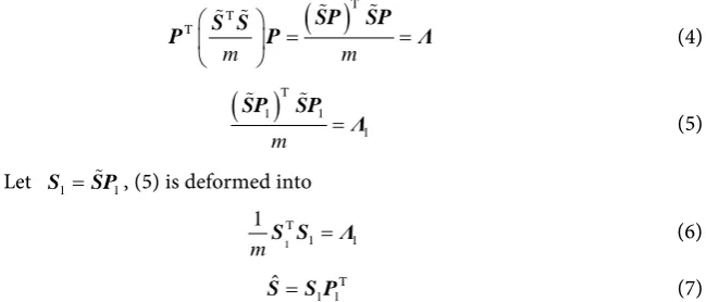
If T

DOI: 10.4236/sgre.2017.812024 369 Smart Grid and Renewable Energy

( )

T

T T m m   = =     SP SP S S

P P Λ

 

 

(4)

( )

T

1 1 1 m = SP SP Λ   (5)

Let S1=SP 1, (5) is deformed into

1

T 1 1 1

mS S = Λ (6)

T 1 1 ˆ₌

S S P (7)

As known from (6), the covariance of the dimensions is zero in the matrix S1. Each row of the matrix S is a sample. Furthermore each column of the matrix

P1 is an eigenvector, and the k eigenvectors of the matrix P1 are orthogonal to each other. So, SP 1 is the equivalent to linear transformation of each sample of S in the basis of column vectors in P₁. After the transform, each row vector of

S1 is completely irrelevant, and the dimension of each sample is k, where

1 m k R × ∈

S . If k < n, then the operation of dimension reduction is completed, while the internal structure of the original data is preserved with the maximum probability. Finally the matrix S can be approximately recovered by (7).

3. PQ Data Compression via IPCA

This section presents a methodology that allows the PQ data compression in smart distribution systems.

3.1. Data Matrix

PQ data from smart distribution systems, need to be acquired and compressed, then transmitted through the communication network to the server of the con-trol center for further analysis. Let the acquired data be put in the form of a ma-trix X, shown in Figure 1. It is convenient to represent the data, and be easily used for data compression. Here each row of X is taken from a distributed mea-surement point at each time instant.

3.2. Data Compression

After the centralization processing of the matrix X, the eigenvectors corresponding to the first k eigenvalues of the covariance matrix C are calculated as the principal components by PCA algorithm. The eigenvectors corresponding to the smaller n-k

[image:4.595.215.540.74.213.2]

eigenvalues are eliminated, and the remaining ones are constructed to the matrix P1. Then the matrix S is transformed into the matrix S1, which the CR is n:k. The

DOI: 10.4236/sgre.2017.812024 370 Smart Grid and Renewable Energy original data can be reconstructed using (7), and the mean square error of the reconstructed data is equal to the sum of the eliminated n-k eigenvalues. How-ever, the main difficulty of data compression based on PCA algorithm is to find the eigenvalues and eigenvectors of the covariance matrix.

At present there are two kinds of conventional methods: one is firstly uses of 0

λI−A = to calculate the eigenvalues of the covariance matrix A, then uses

(

λI−A

)

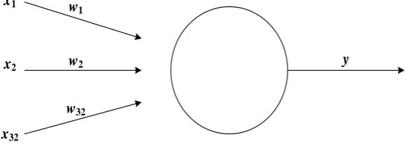
x=0to calculate all the eigenvectors corresponding to the eigenvalues. Because the size of A is generally large, the computation of this method is very large and time-consuming. So it is not suitable for data compression. Another method is realized by using neural network (NN) method. This method is simp-ler than the first method, and does not need to compute the covariance matrix. Taking the 32 samples as an example, the construction of the single-layer NN is illustrated in Figure 2.

The weights of the network are iteratively adjusted and the iterative equation is as follows:

( )

32

( ) ( )

( ) ( )

T

1

i i

i

y k w k x k w k x k

=

=

∑

= (8)

(

)

( )

( ) ( )

2

( ) ( )

1

w k+ =w k + ⋅µ _y k x k −y k w k _ (9)

From Literature [17], finally the w converges to the eigenvector corresponding to the maximum eigenvalue, but its convergence speed is closely related to the learning factor µ. Only while 1

3 2 2

0.8899 2

µλ

≤ − ≈ ₍λ_{1 is the maximum}

eigenvalue of C), (9) can converge to the eigenvector corresponding to the maximum eigenvalue. And while µλ =1 0.618, the convergence speed of (9) is

the fastest.

But λ1 is unknown, so it may lead to poor estimation of the learning factor

µ. If the estimated µ is too small, it will result in slow learning speed. In con-trast, if the estimated µ is too large, it will results in divergence of (9). There-fore the NN method has limitations for the real applications.

[image:5.595.228.523.597.700.2]

In order to solve the above problems, this paper proposes a new method for finding the eigenvectors of the covariance matrix. Firstly, prove a theorem as follows:

Figure 2. Single-layer neural network.

w

1

w

2

w

32

x

1

x

2

x

32

DOI: 10.4236/sgre.2017.812024 371 Smart Grid and Renewable Energy Theorem 1. If

( )

(

(

1

)

)

, 1

n n

Aw k

w k R

w k

× −

= Α ∈

− (10)

where A is a nonnegative symmetric matrix,

( )

1

0 n

w R ×

∀ ∈ _, w

( )

0 is not per-pendicular to the eigenvector corresponding to the largest eigenvalue of A, then

( )

( )

{

}

lim s the eigenvector corresponding to the largest eigenvalue of

k

w k

e e i A

w k

→+∞ ∈

(11) Proof.

_{A is a nonnegative symmetric matrix, where} n n

R ×

∈ A .

(

)

1

1, 2, , , , 1 1,

n

n i

p p p p R × p

∴∃ =P  ∈ = where pi is the eigenvector

cor-responding to the eigenvalue λi, and any two vectors in P are orthogonal. The

matrix P satisfies:

T ₌

P CP Λ (12)

then

( )

1

0 n

w R×

∀ ∈ _{can be linearly expressed by} p_i as follows:

( )

0 1 1 2 2 i i n n

w =a p +a p + + a p + + a p (13)

Since w

( )

0 is not perpendicular to the eigenvector corresponding to the largest eigenvalue of A, then a1 ≠1.

( )

(

(

)

)

( )

( )

( )

1 1 0 1 0 k k

w k w

w k w k

w k −w

−

= ⇒ =

−

A A

A (14)

( )

(

)

( )

1 1 ₁

1 0

k

n n _k

w k a p a p

w −

=A + +

A

 (15)

( )

( )

1 1 1 ₁

1

1 0

k

k n

n n _k

w k a p a p

w λ λ λ −  _{ }    = _ + +   _  

   A (16)

Because A is nonnegativedefinite matrix, let

1 2 i i 1 n 0

λ =λ ==λ >λ₊ ≥≥λ ≥ , then

1

lim 0, 1, , . k

m

k m i n

λ λ →+∞   = = +     

Let 1 1 11 11

1 1

k k

i n

i k i n k n

a p a λ p a λ p

β

λ λ

+ +

+ +

= + + + + , then lim

( )

( )

lim

k k w k w k β β →+∞ = →+∞

1 1 2 2

lim i i,

k→+∞β =a p +a p + +a p i<n

 

( )

( )

11 11 22 22

lim lim i i

k k

i i

w k a p a p a p

a p a p a p

w k β β →+∞ →+∞ + + + ∴ = = + + + 

 (17)

where p p1, 2,piare the eigenvectors corresponding to the largest eigenvalue

1

λ_{, so the sum of them multiplied by a scalar is still the eigenvector} correspond-ing to the largest eigenvalue λ1 of the matrix A.

DOI: 10.4236/sgre.2017.812024 372 Smart Grid and Renewable Energy matrix: firstly calculate the eigenvector e1 corresponding to the largest

eigen-value λ1 using (10), then calculate the eigenvector e2 , because of T

1 n

i i i i

A

λ

e e

=

=

∑

_{, let} T

(

T

)

1 1 1, 1 1 1

B= −A λe e λ =e Ae , so the eigenvalues of B are sorted by size to λ2 ≥≥λk ≥≥λn ≥λn+1 =0. It can be seen that if A is replaced by B, the second principal component can be calculated, and then the other prin-cipal components can be calculated by this method in turn.

The following simplified steps are applied to PQ data compression based on the IPCA:

Step 1. Get PQ data.

Step 2. Calculate the mean of PQ data using (1). Step 3. Subtract the mean from PQ data using (2).

Step 4. Construct the covariance matrix of the subtract data using (3).

Step 5. Calculate eigenvectors and eigenvalues of the covariance matrix using the iterative method.

Step 6. Choose principal components and preserve the k (the desired number) principal components which correspond to the larger eigenvalues.

Step 7: Quantization and encoding: preserve the quantized principal compo-nents and their indices as the compressed coefficients.

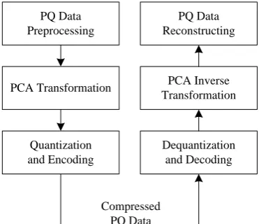
[image:7.595.279.465.527.687.2]

The PQ data compression scheme based on the PCA algorithm is shown in

Figure 3.

4. Data Test, Discussion and Comparison

IPCA and discrete wavelet transform (DWT), both methods are capable of mul-tichannel PQ data compression. PQ data are collected from various measure-ment points in the smart distribution system to test the methods. The PQ data are sampled at 12.8 kHz and quantized with 16 bits. Here there are 32-channel PQ data, and each channel data consists of 1536 samples. The tested PQ matrix is formed as m n

R × , where m is the number of sample channels and n is the number of samples of each channel PQ data. The CR of the proposed method is

Figure 3. PQ data compression scheme based on the PCA algorithm.

PQ Data Preprocessing

PCA Transformation

Quantization and Encoding

PQ Data Reconstructing

PCA Inverse Transformation

Dequantization and Decoding

DOI: 10.4236/sgre.2017.812024 373 Smart Grid and Renewable Energy given as (18). By determining different number of principal components, differ-ent CRs can be obtained.

Number of data without compression Number of data after transformation =

CR (18)

Mean absolute error (MAE) and mean percentage error (MPE) shown as (19) and (20) respectively are used to evaluate the reconstruction accuracy of PQ da-ta.

1

1

ˆ

n

i i

i

MAE x x

n =

=

∑

− ₍₁₉₎

1

ˆ 1

100

n

i i

i i

x x

MPE

n = x

−

=

∑

× ₍₂₀₎

where xˆ_i is the reconstructed data corresponding to the original data xi of

each channel.

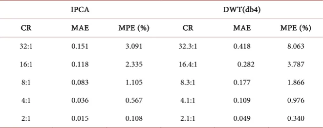
In order to compare the performance of data compression using the IPCA, DWT is proposed to carry out for the compression of the same dataset. Table 1

shows results obtained with the IPCA and with Debaucheries 4 wavelet (db4) and four levels of decomposition [7]. Different thresholds have been set, aiming to retain the number of wavelet coefficients that would result in the same CRs shown for the IPCA.

It can be seen from Table 1 that the IPCA is capable of achieving better tra-deoff for higher CRs. The MAE and MPE of reconstructed data by the IPCA are lower than those of reconstructed data by the DWT. So the performance of data compression using the IPCA is better than that using the DWT.

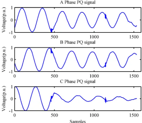
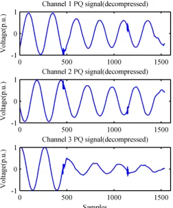
Figure 4 shows the original PQ data of the first three channels. Figures 5-8 il-lustrate the decompressed PQ data of the first three channels, which use the ex-traction of 2, 4, 8 and 16 principal components by the IPCA.

[image:8.595.208.539.589.720.2]

It can be found from Figures 5-8 that while the 2 or 4 or 8 eigenvectors are retained, there is no difference in visual reconstruction effect of the original PQ data. The CR can be as high as 8, and the more the principal components are ex-tracted, the better the reconstruction effect is. But when the CR arrives with 16, it may lead to serious distortion of the reconstructed data.

Table 1. Performances comparison of IPCA and DWT (db4).

IPCA DWT(db4)

[image:9.595.253.496.75.285.2] [image:9.595.252.500.324.610.2]

DOI: 10.4236/sgre.2017.812024 374 Smart Grid and Renewable Energy Figure 4. The original PQ data of the first three channels.

Figure 5. The reconstructed PQ data of the first three channels (CR = 2).

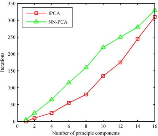
Figure 9 shows a comparison of the number of iterations for calcu-lating their principal components of the tested PQ matrix by the IPCA and NN-PCA. The horizontal axis is the number of eigenvectors and the vertical axis is the number of iterations. It can be found from Figure 9

[image:10.595.250.498.74.357.2]

DOI: 10.4236/sgre.2017.812024 375 Smart Grid and Renewable Energy Figure 6. The reconstructed PQ data of the first three channels (CR = 4).

[image:10.595.254.507.395.699.2]

[image:11.595.256.503.75.367.2]

DOI: 10.4236/sgre.2017.812024 376 Smart Grid and Renewable Energy Figure 8. The reconstructed PQ data of the first three channels (CR = 16).

Figure 9. Comparison about the number of iterations by the IPCA and NN-PCA.

[image:11.595.246.513.403.633.2]

DOI: 10.4236/sgre.2017.812024 377 Smart Grid and Renewable Energy

5. Conclusions

In summary, the benefits of PCA algorithm are used to reduce the redundancy of data. Because PCA algorithm is the optimal transform with the minimum mean square error, according to the requirements, the larger eigenvalues are re-served, and the smaller eigenvalues are omitted to reduce the dimensionality, simplify the model or compress the data. With these characteristics, PCA algo-rithm can be applied to be good for data compression. This paper proposes a multichannel PQ data compression algorithm via IPCA. PQ data is preprocessed to form the matrix. Then IPCA is used to compress the matrix and yields the compressed data. Field PQ data tests validate that the proposed method is cha-racterized with high CR, accurate reconstruction, and low computation plexity. And the iterative method is especially easy to be programmed in com-puter.

Because the test data is not particularly sufficient, and there are differences of the covariance matrices of the original data, the number of iterations will appear very different using the proposed method. The number of iterations has a great relationship with the construction of the initial vector. How to construct the ini-tial vector and reduce the number of iterations according to the different PQ da-ta needs further study.

Acknowledgements

This work is supported by National Natural Science Foundation of China (No. 51477124).

References

[1] Heydt, G.T. (2010) The Next Generation of Power Distribution Systems. IEEE-Transactions on Smart Grid, 1, 225-335. https://doi.org/10.1109/TSG.2010.2080328 [2] McBee, K.D. and Simoes, M.G. (2012) Utilizing a Smart Grid Monitoring System to

Improve Voltage Quality of Customers. IEEE Transactions on Smart Grid, 3, 738-743. https://doi.org/10.1109/TSG.2012.2185857

[3] Li, S. and Wang, X. (2015) Cooperative Change Detection for Voltage Quality Mon-itoring in Smart Grids. IEEE Transactions on Information Forensics and Security, 11, 86-99. https://doi.org/10.1109/TIFS.2015.2477796

[4] Tcheou, M.P. and Lovisolo, L. (2014) The Compression of Electric Signal Wave-forms for Smart Grid: State of the Art and Future Trend. IEEE Transactions on Smart Grid, 5, 291-304. https://doi.org/10.1109/TSG.2013.2293957

[5] Cormane, J. and Astonishment, F. (2015) Spectral Shape Estimation in Data Com-pression for Smart Grid Monitoring. IEEE Transactions on Smart Grid, 7, 1214-1221. https://doi.org/10.1109/TSG.2015.2500359

[6] Unterweger, A. and Engel, D. (2015) Resumable Load Data Compression in Smart Grids. IEEE Transactions on Smart Grid, 6, 919-929.

https://doi.org/10.1109/TSG.2014.2364686

DOI: 10.4236/sgre.2017.812024 378 Smart Grid and Renewable Energy [8] Meher, S.K., Pradhan, A.K. and Panda, G. (2004) An Integrated Data Compression

Scheme for Power Quality Events Using Spline Wavelet and Neural Network. Elec-tric Power System Research, 69, 213-220. https://doi.org/10.1016/j.epsr.2003.10.001 [9] Norman, C.F.T. and John, Y.C.C. (2012) Real-Time Power-Quality Monitoring with

Hybrid Sinusoidal and Lifting Wavelet Compression Algorithm. IEEE Transactions on Power Delivery, 27, 1718-1726. https://doi.org/10.1109/TPWRD.2012.2201510 [10] Ning, J., Wang, J., Gao, W. and Liu, C. (2011) A Wavelet-Based Data Compression

Technique for Smart Grid. IEEE Transactions on Smart Grid, 2, 212-218. https://doi.org/10.1109/TSG.2010.2091291

[11] Zhang, M., Li, K.C. and Hu, Y.S. (2011) A High Efficient Compression Method for Power Quality Applications. IEEE Transactions on Instrumentation and Measure-ment, 60, 1976-1985. https://doi.org/10.1109/TIM.2011.2115590

[12] He, S.F., Zhang, M., Tian, W., Zhang, J. and Ding, F. (2015) A Parameterization Power Data Compress Using Strong Trace Filter and Dynamics. IEEE Transactions on Instrumentation and Measurement, 64, 2636-2645.

https://doi.org/10.1109/TIM.2015.2416451

[13] Souza, J.C.S. de, Assis, T.M.L. and Pal, B.C. (2015) Data Compression in Smart Dis-tribution Systems via Singular Value Decomposition. IEEE Transactions on Smart Grid, 6, 275-284.

[14] Draper, B.A., Baek, K., Bartlett, M.S. and Beveridgea, J.R. (2003) Recognizing Faces with PCA and ICA. Computer Vision and Image Understanding, 91, 115-137. https://doi.org/10.1016/S1077-3142(03)00077-8

[15] Ding, Q. and Kolaczyk, E.D. (2010) A Compressed PCA Subspace Method for Anomaly Detection in High-Dimensional Data. IEEE Transactions on Information Theory, 59, 7419-7419. https://doi.org/10.1109/TIT.2013.2278017

[16] Liu, Y. and Pados, D.A. (2016) Compressed-Sensed-Domain L1-PCA Video Sur-veillance. IEEE Transactions on Multimedia, 18, 351-363.

https://doi.org/10.1109/TMM.2016.2514848