Procedure to Evaluate the Impact in Distribution Single Phase Transformers, Due to Massive Insertion of New Nonlinear Load, Which Changes Daily Demand Graphs

Procedure to Evaluate the Impact in Distribution

Single Phase Transformers, Due to Massive

Insertion of New Nonlinear Load, Which Changes

Daily Demand Graphs

Jorge Enrique Carrión González 1,_{*,Antonio Martínez García} 2_{,Alfredo del Castillo Serpa} 2_, Marianela Carrión González 3, Rodolfo Pabel Merino 3 and Kelvin Alulima Carrión 1

1 _{Nacional University of Loja. Electromechanical Engineering Degree. Loja, Ecuador}

2 _{Technological University of Habana “José Antonio Echeverría”. Electrical Engineering department. La} Habana, Cuba.

3 _{Nacional University of Loja. Electronics and Telecommunications Engineering Degree. Loja, Ecuador.}

*Correspondence: [email protected]/[email protected]; Tel. +593-99-4448995

Abstract: Power Electronic development determines introduction of nonlinear devices in Electric Power Systems. Introduction of nonlinear devices increase current harmonics in Transmission and Distribution Power Systems. Distribution transformers and feeders increase power losses and their nominal parameters are reduced. Present work introduces a procedure to evaluate maximum permissible load in single phase distribution transformers with massive introduction of a new type of nonlinear load which changes daily demand graphs.

Keywords:current harmonics; stray losses; statistical inference; daily demand graphs

1. Introduction and Background

The impetuous development of Power Electronics has led to the massive introduction of “Flexible Alternating Current Transmission Systems” (FACTS) in Transmission Networks. Household appliances and computer equipment that are based on applications of this discipline are growing in homes. Electric vehicles are being imposed over internal combustion vehicles, which imply an increase in charging stations that are also based on Power Electronics. The abovementioned results in harmonic currents increases in transmission and distribution networks. Current harmonics produce additional windings heating, due to stray losses caused by Eddy currents. Stray losses determine the level of decreasing the rated current for risen harmonics, according to the standard ANSI/IEEE C.57.110 [1,2,3,4,5]. This situation explains the increases in temperature, above nominal values, in transformers that feed non linear loads, even when the fundamental load current is below it nominal value, exposing it to premature failures. The transformers, until a few years ago, were designed to operate under sinusoidal conditions at the source and / or the load, but in practice, the presence of harmonics caused by non linear loads, such as electronic equipment and rectifiers, is a form of current pollution that cause problems if the effective harmonics current increases above certain limits [2,5,6,7,8].

Additionally, the massive introduction of new types of non linear loads, that modify the typical daily current demand graph, makes an evaluation of transformers heating state necessary to timely decision making.

2. Materials and Methods

In recent works [9,10,11,12,13] it has not been possible to obtain a procedure to evaluate the impact of massive introduction of new types of non linear loads in single phase distribution transformers, without measure of the fundamental current and its harmonics, in the previous hours and at the peak. If a representative database of the fundamental secondary currents and its harmonics is available, in distribution transformers during a week, it is possible to estimate hourly typical demand and harmonic loss constants, that allow, from a measurement or estimate of the fundamental current at the peak, estimation of transformer heating state without measurements of fundamental current and its harmonics during all day hours. The previous assumption presupposes homogeneity throughout analyzed period. To undertake this task, it is necessary:

a) Characterize the typical demand graph when different quantities of a type of polluting loads are introduced.

b) Identify average values of the harmonic losses factors in conductors during the different hours of the day(FHL) and in other parts of the transformer (FHL-STR) and

their confidence intervals.

c) Identify the typical hourly graph of harmonics effective current and it confidence interval when different quantities of a new type of polluting loads are introduced. d) Estimate, with the information in subsections a, b and c, initial heating state of the

transformer when the Electric Peak begins.

e) Once the fundamental peak load and ambient temperature are known or estimated, calculate the actual heating state of the transformer so that the temperature of the hottest point does not exceed the limit temperature according to its insulation class, to contribute to timely decision making.

Additionally, it is necessary to take into account some assumptions and considerations already established among which are:

a) It is assumed with some foundation, that all consumers of the identified population have a potential for installed equipments (not including new pollutant loads) that cause a similar behavior of current harmonics. That means that their behavior is a variable randomized with normal distribution in each hourly time interval.

b) The influence of iron losses on the additional heating suffered by the single-phase distribution transformer in the presence of non linear loads is considered negligible. c) The heating of the distribution transformers is a slow physical phenomenon, given their

high thermal inertia, which causes them to reach their highest temperature some time after the period of higher overload.

It is also important to estimate the value of the highest temperature that reaches the hottest point of the transformer [14,15,16,17], since this is an important indicator that determines its operational life span. The value of the maximum temperature reached by the transformer depends not only on the overload to which it is subjected, but also on it heating state before the overload occurs which is clear in the IEEE C57.110 [1,2,4,18], where it is advisable to consider as a state prior to the overload, the one corresponding to 12 hours before this overload takes place.

Heating is due to the heat generated internally for two fundamental causes: losses in iron and losses due to Joule and stray effect in windings and other parts of transformers [11,18,19].

In the vast majority of international works, [9,11,12,18,19,20] the transformers heating state is calculated only in one hour, given the connected load and known the harmonic composition of the current. In the present work it is not known how influences, the introduction of a new type of polluting load, in the typical demand graph and how change, hour by hour, the harmonic composition of the current. This paper is based on a procedure to solve the aforementioned problems, which is summarized in a synthesized way below.

2.1. Proposed procedure

1. Characterize the population. 2. Select a representative sample.

3. Obtain the typical daily current demand graph in transformers, due to the inclusion of a new type of polluting load.

4. Identify homogeneous groups of transformers (by capacity and number of users with polluting loads) considering the effective harmonics current as a normally distributed random variable.

5. Characterize harmonic losses factors FHL and FHL-STR according to the groups

determined in step 4.

6. Identify an appropriate variable of loading state of each transformer (Intensity of fundamental current in the peak), that can be measured or estimated to decode to natural values the typical graphs of fundamental and harmonics effective current corresponding to analyzed transformer and perform the calculation of its equivalent heating state. Estimate result´s confidence intervals.

2.2. Proposed procedure description

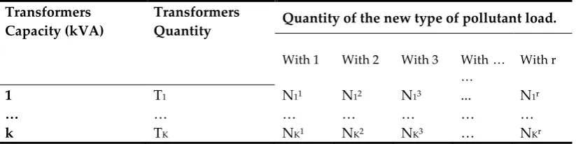
Step 1: Distribution subsystem characterization related with those transformers that have associated new type of polluting loads. This characterization corresponds to the total population of transformers that have consumers associated with this type of loads. This step concludes with Table 1.

Table 1. Subsystem characterization with a new type of polluting load.

Transformers

Capacity (kVA) Transformers Quantity Quantity of the new type of pollutant load. With 1 With 2 With 3 With …

… With r

1 T1 N11 N12 N13 ... N1r

… … … …

k TK NK1 NK2 NK3 … NKr

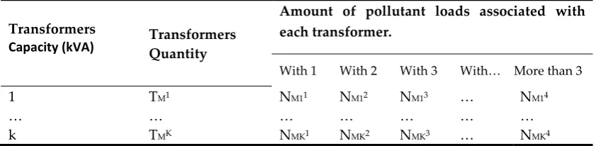
Table 2. Representative sample of the total population of transformers with new types of pollutant loads.

Transformers

Capacity (kVA) Transformers _Quantity

Amount of pollutant loads associated with each transformer.

With 1 With 2 With 3 With… More than 3

1 TM1 NM11 NM12 NM13 … NM14

… … … …

k TMK NMK1 NMK2 NMK3 … NMK4

Step 3: Analyze, according to fundamental current intensity, the base days for obtaining a characteristic daily current demand. The hourly graphs of the fundamental current component are constructed in per unit of the days of the week, based on measurements of all the transformers of the sample. The base in each day corresponds to the highest fundamental effective current intensity in the peak in each day, because what matters is the shape of the demand daily graph. Compare the graphs obtained and verify the random hourly behavior (if necessary) and select the most representative day or days in the transformer heating. These selected days are used to obtain the desired characteristic day.

Step 4: Homogeneous groups for the base day or days obtained from the previous step (classes) are identified, to obtain typical curves of average values of harmonics effective current. In this case, it is necessary to verify that the groups comply with the normal distribution law at each time interval.

Step 5: Evaluate for the base day or days obtained from step 4, the average values of harmonic factors FHL and FHL-STR in each hourly interval for each homogeneous group (classes). In this case it is necessary to verify that the groups comply in each hourly interval with the normal distribution law. At the end of this step you have the information of the hourly average harmonics effective currents and harmonics factors FHL and FHL-STR for each selected class.

Step 6: For each transformer identify a suitable value to decode the fundamental and harmonics effective current intensity to natural values. With the results of the previous step, the database for equivalent heating state calculation of all transformer groups is ready. Note that each transformer is associated with only one grouping or class.

3. Results.

As of 2010, the Ministry of Energy of Ecuador has implemented a massive replacement plan for gas cooking with induction cookers. The average demand per user of this type of cooker has been estimated at 2.4 kW [21,22]. This decision causes important changes in the typical demand graph for residential consumers in the hours of breakfast, lunch and dinner, as well as the increase in current harmonics circulation in transformers and distribution feeders.

3.1. Application of the procedure to the case of Loja City, Ecuador.

Step1: This characterization corresponds to the total population of transformers that have consumers associated with induction cookers. The information is sorted according to Table 3 from the database processing.

Table 3. Number of cookers per transformer capacity. Transformers

Capacity (kVA) Transformers Quantity Number of cookers per transformer With 1 With 2 With 3 More than 3

10 30 20 10 0 0

15 32 18 10 2 2

25 90 40 22 15 13

37,5 45 18 9 13 5

Step 2: From the previous characterization, a representative sample of transformers with induction cookers is selected see Table 4.

Table 4. Transformers sample with induction cookers.

Transformers Capacity (kVA)

Transformers Quantity

Number of cookers per transformer.

With 1 With 2 With 3 More than 3

10 20 15 5 0 0

15 20 11 5 2 2

25 78 34 16 15 13

37,5 34 14 5 10 5

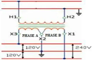
Step 3: Fundamental load current behavior of each transformer capacity in the week is analyzed in order to obtain the base days required to calculate the characteristic day in the two phases of the transformer. Phases A and B are considered the terminals of the secondary winding with central tap (figure 1). In the analyzed case, there are no substantial differences in consumption in the winter and summer months, only slightly lower ambient temperatures in the first case, that’s why the used database was for the entire year. The simple inspection method is used as an initial variant to identify potential groupings of days with respect to the average intensity during the day. Of course, this analysis is carried out in the two phases of the transformer independently.

The hourly demand graphs of the fundamental current intensity are constructed in per unit with respect to the maximum of the corresponding day, based on the measurements provided by the E.E.R.S.S.A. The results are presented in Figure 2.

Figure 2. Hourly demand graphs of the fundamental effective currents.

Comparing the graphs, two potential groupings are evident. That is, the group from Monday to Friday and the group from Saturday and Sunday. Hypothesis tests are carried out with a significance level of 0.05, verifying that the aforementioned groups are different and weekdays can be considered as a homogeneous group [23,24].

According to the statistical analysis carried out, it is concluded that the average demand on weekends are lower than the average demand from Monday to Friday, so the worsts days for transformer heating are the days during the week. These average values during the week from Monday to Friday will be considered to evaluate transformer heating, since it is additionally known that the daily peak values, to express the demand in per unit, are kept lower on weekends than on weekdays.

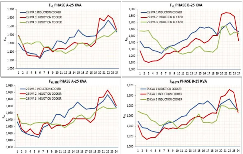
Step 4: When the same data is used by grouping all transformers with any number of cookers to calculate the typical daily demand graph of harmonics effective current, based on the maximum value of the fundamental component in each day, very similar results are obtained in the shape of the curve, with slightly higher values as shown in figure 3. However, when the compliance with the normal distribution law is checked in each time hourly interval, it is not met, so in this case is investigated new grouping by capacity with the same number of cookers.

The results obtained for the 25 kVA transformers with different number of cookers in both phases are shown in Figure 4.

Figure 4. Typical graphs of effective harmonics currents in 25 kVA transformers with different number of induction cookers.

Next, it is checked for each grouping at all time intervals and for all capacities, compliance with the normal distribution law for effective harmonics current. The goodness of fit tests used to check normality were Kolmogorov-Smirnov, Chi square and Anderson Darling with a P value greater than 0.1. The results were positive in all cases [1,4,23,24,25].

Step 5: The factors FHL (Harmonic loss factor for Eddy current losses) and FHL-STR (Harmonic loss factor for other stray losses) are calculated in each hour [1,7,26], for each phase, of each group Figure 5, and the similarity tests of average values and normality are carried out at all time intervals of the groupings made in the previous step using the same goodness fit test with the same value of P, with positive results [1,23,24].

Step 6: In this step, the transformers fundamental currents intensity must be decoded to find physical values in per unit with respect to the nominal values of the transformer.

Known the typical fundamental daily current demand graph and the peak current demand, it is always possible to estimate the rest of the values for the different hours of the day.

The same happens with the typical graphs of effective harmonics current that was calculated on the same basis as the fundamental one, so at any time considered it is possible to know the relationship between these two values and their real values from the measurement or estimation of the fundamental peak current intensity. After this step it is possible to perform the calculations to any specific case.

3.2 Calculations for a specific case of a 25 kVA transformer.

A 25 kVA transformer with one cooker in the interval 19H00 to 20H00 is analyzed. The characteristic values of transformer losses in per unit (referred to PDC), are presented in Table 5.

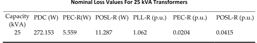
Table 5. Nominal losses in 25kVA, INATRA transformers.

Nominal Loss Values For 25 kVA Transformers

Capacity

(kVA) PDC (W) PEC-R(W) POSL-R (W) PLL-R (p.u.) PEC-R (p.u.) POSL-R (p.u.)

25 272.153 5.559 11.287 1.062 0.0204 0.0415

5 _{Source: INATRA Transformer Factory Test Protocol.}

Where:

PLL-R: Nominal copper losses at 60 Hz.

PEC-R: Losses due to eddy 60 Hz currents in conductors.

POSL-R: Losses due to 60 Hz current in other parts of the transformer. PDC: Nominal Copper losses.

If the fundamental current intensity in phases A and B in the secondary,

I

fA and

I

fB, are measured in p.u. referred to the nominal current in the time interval considered, it is possible to estimate:

 From the typical current curves shown in Figure 4, the average values of the harmonic effective current intensities of both phases: IefhA and

I

efhB and their confidence intervals in

p.u. referred to the nominal current of the transformer.

 The mean values of the stray loss factors FHLA, FHLB, FHL-STRA and FHL-STRB of phases A and B, and their confidence intervals calculated in step 5.







 

















 







2 2

max _{2 2}

2

1 1

2

fA fB LL R

efhA HLA EC R STRA OSL R efhB HLB EC R STRB OSL R

I I P I

I F P FHL P I F P FHL P

                             

 

₍₁₎

Considering the three variables in equation (1) (FHL, FHL-STR and Ief) not dependents, it is possible to calculate the upper bound error of Imax calculation using equation (1) as:



 

















 







0,5

2 2 2 2

max 1,5 2 2 2 2 0,5 1 1 2

fhA fhB fA fB

LL R EC R

ef HL

efhA HLA EC R HL STRA OSL R efhB HLB EC R HL STRB OSL R

I I I I

P P

I F

I F P F P I F P F P

            _  _         _{        }      _{ }  



 

















 







0,5

2 2 2 2

1,5

2 2

0,5

2

2

1

.

1

2

fhA fhB fA fB

LL R OSL R

HL STR

efhA HLA EC R HL STRA OSL R efhB HLB EC R HL STRB OSL R

I

I

I

I

P

P

F

I

F P

F

P

I

F

P

F

P

        















_





_

















































_

_









 

















 









 

















 







0,5 2 2 1,5 2 2

1

1

2

0,5

1

1

2

fA fB

LL R efhA HLA EC R HL STRA OSL R efhB HLB EC R HL STRB OSL R

efhA HLA EC R HL STRA OSL R efhB HLB EC R HL STRB OSL R

I

I

P

I

F P

F

P

I

F P

F

P

Ief

I

F P

F

P

I

F P

F

P

            









































 







_

_

_

_

_

_

_

_

_



















_

_







(2)

The upper level of the error is ensured by taking in equation (2) the highest values of

∆𝐹

𝐻𝐿

,

∆𝐹

and

∆𝐼𝑒𝑓

of phases A and B, calculated with a 95% confidence level.

Equation (2) is obtained by differentiating equation (1). Evaluating the heating state in p.u. with respect to nominal conditions in the interval 19H00 to 20H00 (PLLTh-Peak), using equation (3), for a 25 kVA transformer with one induction cooker of Chontacruz feeder in Loja, which has average pick demand values: IfA= 0.622 p.u., IfB = 0.63 p.u., and IefhA= 0.634 p.u., IefhB= 0.65 p.u., results in:



 

















 







2 2

P 1 1

LLTh eak efhA HLA EC R HL STRA OSL R efhB HLB EC R HL STRB OSL R

P _ I  F P _ F _ P _ I  F P _  F _ P _

(3)

0.441 . .

LLTh Peak

P

_



p u

This represents 5.8% more losses due to harmonic currents, or equivalent to the fundamental current intensity of the transformer being 2.86% higher. From equations (1) and (2) for these loading conditions:

max

maxef max I ef

0.971 0.009 . .

p u

Based on upper results 25 kVA transformers with one induction cooker, for the analyzed peak demand lose almost 3% of their capacity. Calculation confidence level is 95%.

3.3 Transformer heating estimation in a load cycle.

The objective of the developed procedure is the evaluation of transformers heating during a load cycle, not transformer nominal declassification in a certain time interval. For this, it is not necessary to use the expression that allows declassification evaluation (1) due to current harmonics, but it is required estimation of the previous heating before the peak, and with this value and the heating during the peak, evaluate if the transformer can reach temperatures at the hottest point above what allows its thermal insulation. The preheating can be estimated as:



 

















 







2 2

14 Pr

1

1 1

(2 )

efhA HLA EC R HL STRA OSL R efhB HLB EC R HL STRB OSL R LLTh evious

i

I F P F P I F P F P

P

N

     





          

 



  

 



(4)

Where:

I . I : Effective harmonics currents in phases A and B in the time interval i.

F , F , F , F : Harmonic loss factors of phases A and B in the time interval i. N: is the number of previous time intervals considered.

In this case, 14 hours are taken to account for previous heating due to the use of induction cookers for breakfast. During the peak, transformer heating state is estimated with expressions similar to the previous ones, but only averaging the number of hours the peak occurs.

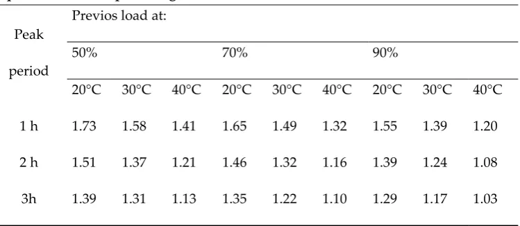
Considering the previous state of heating before the peak and during the peak and the ambient temperature, it is possible to determine using the information in Table 6 [7,16,17,18,27], if that overload is less than the maximum that the transformer can withstand without exceeding the temperature at the hottest point the maximum allowed.

Table 6. Allowable peak overloads to select the capacity of oil-cooled transformers. Allowable peak overloads to select the capacity of the oil-cooled transformers, equivalent load in percentage of the nominal.

Peak

period

Previos load at:

50% 70% 90%

20°C 30°C 40°C 20°C 30°C 40°C 20°C 30°C 40°C

1 h 1.73 1.58 1.41 1.65 1.49 1.32 1.55 1.39 1.20

2 h 1.51 1.37 1.21 1.46 1.32 1.16 1.39 1.24 1.08

3h 1.39 1.31 1.13 1.35 1.22 1.10 1.29 1.17 1.03

8 _{Source: Distribution Transformers. Dr. Héctor Silvio Llamo Laborí.}

row the average ambient temperature at analyzed heating time interval and in the rest of the rows relates the overload values to which the transformer can be subjected during the peak period without any danger of a decrease in its operational life span. Under specific manufacture’s information it is convenient to carry out calculations based on that information and not from Table 6.

3.4 Calculation of the 25 kVA transformer heating state with one cooker in a load cycle.

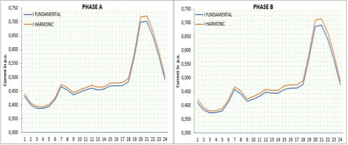
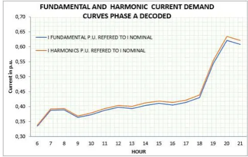
If the same 25 kVA transformer is considered with one induction cooker in the Chontacruz feeder in Loja City with known typical fundamental and harmonics standardized current demand graphs in both phases (Shown in Figure 6A for phase A) and its corresponding decoded graphs (Shown in Figure 6B for phase A), it is possible by applying equation (4), in the 14 hours prior to the peak, to determine the transformer heating state prior to the period of greatest demand. By proceeding in a similar manner with the three hours that the peak lasts equation (5), the heating state to which the transformer is subjected in this period can be estimated. If the proposed procedure is applied, the following results are reached:

Pr

0.276 . .

LLTh ior

p u

P





Figure 6A. Current daily typical standardized demand graphs for Phase A.

Figure 6B. Decoded daily current demand graphs for phase A. (p.u. respect to I nominal).



 

















 







2 2

3

P 1

1 1

(2 3)

efhA HLA EC R HL STRA OSL R efhB HLB EC R HL STRB OSL R

LTh eak

i

I F P F P I F P F P

P _      



          

 



  

 

0.3838 . .

LTh peak

P

_



p u

 Equivalent pre-peak load state = (0.276)0.5 _{p.u. = 0.525 p.u.}

 Transformer peak load state = (0.3838)0.5 _{p.u. = 0.628 p.u.}

 Confidence interval in the determination of the loading state of the transformer using equation (2), at the peak equal to: 0.009 p.u.

In Table 6 [8,18,27,28,29,30] with a 52.5% pre-peak load state (related to nominal) and extrapolated for three hours and 21˚C of ambient temperature [31], the transformer should withstand, without reaching the maximum permissible temperature in the hottest point a 37.2% overload. The error in the estimation is in the order of 0.9%. It can be concluded that the safe peak overload limit for this transformer is 36.3%. It is evident that in this case the transformer with a 95% of confidence level is not in danger of diminishing its operational life span.

4. Discussions of the Results

Proceeding in the same way with the rest of the transformers from the measurement or estimation of the fundamental load at the peak, it is possible to evaluate the maximum overload that the transformer can allow without breaking the regulations to preserve its operational life span. The above results are essential to determine when it is necessary to replace distribution single phase transformers in any feeder according to the number of installed pollution loads. In the same way, under procedure’s assumptions fulfillment it is possible to project to the future.

Proposed procedure allows, with simple measurements of fundamental peak currents at phases A, B and ambient temperature, real time determination of the loading states of transformers and its confidence intervals.

5. Conclusions

Developed procedure allows, on the basis of the statistical processing of harmonic currents measurements in distribution single phase transformers, to determine magnitudes and levels of errors necessary to evaluate their heating states.

From the measurement or estimation of the fundamental current intensity at the peak in the secondary of the distribution transformers, its average heating state is estimated in a load cycle, as well as the upper load level allowed in the peak to reduce risks of thermal isolation damage.

Developed procedure allows estimation of the effect that causes, in a load cycle, the massive introduction of a type of polluting load in the heating state of single phase distribution transformers, when these loads modify the typical demand graphs, contributing to make decisions about the current and future exploitation of transformers.

The application of the methodology to the particular case of Loja City validates the real possibility of its application.

Funding: This research received no external funding.

Conflicts of Interest: The authors declare no conflict of interest.

References

[1] IEEE. IEEE Recommended Practice for Establishing Transformer Capability When Supplying Nonsinusoidal Load Currents. IEEE Std C57110, 2004. 1-3.

[2] IEEE. IEEE Recommended Practice for Establishing Transformer Capability When Supplying Non-sinusoidal Load Currents. ANSI IEEE Std C57110, 1986. 110, 1.

[3] T. Dao, B. T. Phung, y T. Blackburn. Effects of voltage harmonics on distribution transformer losses. In 2015 IEEE PES Asia-Pacific Power and Energy Engineering Conference (APPEEC), 2015. 1-5.

[4] R. D. Henderson y P. J. Rose. Harmonics: the effects on power quality and transformers. IEEE Trans. Ind. Appl, 1994. 30, 528-532.

[5] S. B. Sadati, A. Tahani, B. Darvishi, M. Dargahi, y H. yousefi. Comparison of distribution transformer losses and capacity under linear and harmonic loads. In 2008 IEEE 2nd International Power and Energy Conference, 2008. 1265-1269.

[6] S. B. Sadati, A. Tahani, B. Darvishi, M. Dargahi. Comparison of distribution transformer losses and capacity under linear and harmonic loads. In 2008 IEEE 2nd International Power and Energy Conference, 2008. 1265-1269.

[7] S. Taheri, H. Taheri, I. Fofana, H. Hemmatjou, y A. Gholami. Effect of power system harmonics on transformer loading capability and hot spot temperature. In 2012 25th IEEE Canadian Conference on Electrical and Computer Engineering (CCECE), 2012. 1-4.

[8] L. W. Pierce. IEEE Recommended Practice for Establishing Liquid-Immersed and Dry-Type Power and Distribution Transformer Capability When Supplying Non sinusoidal Load Currents, 2018. 1-68.

[9] D. M. Said y K. M. Nor. Effects of harmonics on distribution transformers. In 2008 Australasia Universities Power Engineering Conference, 2008. 1-5.

[10] A. C. Delaiba, J. C. de Oliveira, A. L. A. Vilaca, y J. R. Cardoso. The effect of harmonics on power transformers loss of life. In 38th Midwest Symposium on Circuits and Systems. Proceedings, 1995. 2, 933-936.

[11] J. Gómez-Sarduy, E. Quispe, R. Reyes-Calvo, V. Sousa-Santos, y P. Viego-Felipe. Corriente sobre las pérdidas en los transformadores, 2014. 45, 33-43.

[12] T. Dao, B. T. Phung, y T. Blackburn. Effects of voltage harmonics on distribution transformer losses. In 2015 IEEE PES Asia-Pacific Power and Energy Engineering Conference (APPEEC), 2015. 1-5.

[13] S. F. Abdelsamad, W. G. Morsi, y T. S. Sidhu. Probabilistic Impact of Transportation Electrification on the Loss-of-Life of Distribution Transformers in the Presence of Rooftop Solar Photovoltaic. IEEE Trans. Sustain. Energy, 2015. 6, 1565-1573.

[14] A. Elmoudi, M. Lehtonen, y H. Nordman. Effect of harmonics on transformers loss of life. In Conference Record of the 2006 IEEE International Symposium on Electrical Insulation, 2006. 408-411. [15] M. A. Awadallah, T. Xu, B. Venkatesh, y B. N. Singh. On the Effects of Solar Panels on Distribution Transformers. IEEE Trans. Power Deliv, 2016. 31, 1176-1185.

[16] S. A. El-Bataway y W. G. Morsi. Distribution Transformer’s Loss of Life Considering Residential Prosumers Owning Solar Shingles, High-Power Fast Chargers and Second-Generation Battery Energy Storage. IEEE Trans. Ind. Inform, 2019. 15, 3, 1287-1297.

[17] J. W. Stahlhut, G. T. Heydt, y N. J. Selover. A Preliminary Assessment of the Impact of Ambient Temperature Rise on Distribution Transformer Loss of Life. IEEE Trans. Power Deliv, 2008. 23, 2000-2007. [18] O. A. Amoda, D. J. Tylavsky, G. A. McCulla, y W. A. Knuth. Acceptability of Three Transformer Hottest-Spot Temperature Models. IEEE Trans. Power Deliv. 2012. 27, 13-22.

[19] M, Daghrah. Experimental investigation of hot spot factor for assessing hot spot temperature in transformers. In 2016 International Conference on Condition Monitoring and Diagnosis (CMD), 2016. 948-951.

[20] S. N. Makarov y A. E. Emanuel. Corrected harmonic loss factor for transformers supplying nonsinusoidal load currents. In Ninth International Conference on Harmonics and Quality of Power. Proceedings (Cat. No.00EX441), 2000, 1, 87-90.

[22] T. Gonen, Electric Power Distribution Engineering, 3a ed. CRC Press, 2014, 4, 100-102.

[23] Murray R, S., & Larry J, S. Estadistica Shaum.4a ed, MEXICO: MC GRAW GRILL. 2004, 3, 94-97. [24] Ronald E. Walpole. Probabilidad y estadística para ingeniería y ciencias, 9a ed, Texas, 2012, 172-174. [25] G. W. Massey. Estimation methods for power system harmonic effects on power distribution transformers. IEEE Trans. Ind. Appl, 1994. 30, 485-489.

[26] A. Elmoudi, M. Lehtonen, y H. Nordman. Effect of harmonics on transformers loss of life. In Conference Record of the 2006 IEEE International Symposium on Electrical Insulation, 2006. 408-411. [27] S. Llamo Laborí. Sistemas Eléctricos de Distribución. Universidad Tecnológica de La Habana. Edición 2010. 513-516.

[28] IEEE. IEEE Standard for General Requirements for Liquid-Immersed Distribution, Power, and Regulating Transformers. 2015.

[29] C. Lopez, M. J. Rider, y Q. Wu. Parsimonious Short-Term Load Forecasting for Optimal Operation Planning of Electrical Distribution Systems. IEEE Trans. Power Syst, 2019. 34, 1427-1437.

[30] K. Najdenkoski, G. Rafajlovski, y V. Dimcev. Thermal Aging of Distribution Transformers According to IEEE and IEC Standards, 2007. 1-5.