Sketching for sequential change point detection

R E S E A R C H

Open Access

Sketching for sequential change-point

detection

Yang Cao

, Andrew Thompson

, Meng Wang

and Yao Xie

Abstract

We present sequential change-point detection procedures based on linear sketches of high-dimensional signal vectors using generalized likelihood ratio (GLR) statistics. The GLR statistics allow for an unknown post-change mean that represents an anomaly or novelty. We consider both fixed and time-varying projections, derive theoretical approximations to two fundamental performance metrics: the average run length (ARL) and the expected detection delay (EDD); these approximations are shown to be highly accurate by numerical simulations. We further characterize the relative performance measure of the sketching procedure compared to that without sketching and show that there can be little performance loss when the signal strength is sufficiently large, and enough number of sketches are used. Finally, we demonstrate the good performance of sketching procedures using simulation and real-data examples on solar flare detection and failure detection in power networks.

Keywords: Change-point detection, Streaming data, Sketching, Anomaly detection, Statistical signal processing

1 Introduction

Online change-point detection from high-dimensional streaming data is a fundamental problem arising from applications such as real-time monitoring of sensor net-works, computer network anomaly detection, and com-puter vision (e.g., [2, 3]). To reduce data dimensionality, a conventional approach issketching(see, e.g., [4]), which performs random projection of the high-dimensional data vectors into lower-dimensional ones. Sketching has now been widely used in signal processing and machine learn-ing to reduce dimensionality and algorithm complexity and achieve various practical benefits [5–11].

We consider change-point detection using linear sketches of high-dimensional data vectors. Sketching reduces the computational complexity of the detection statistic from O(N) to O(M), where N is the original dimensionality and Mis the dimensionality of sketches. Since we would like to perform real-time detection, any reduction in computational complexity (without incur-ring much performance loss) is highly desirable. Sketching

*Correspondence:yao.xie@isye.gatech.edu

This paper was presented [in part] at the GlobalSIP 2015 [1].

1_{H. Milton Stewart School of Industrial and Systems Engineering, Georgia} Institute of Technology, Atlanta, GA, USA

Full list of author information is available at the end of the article

also offers practical benefits. For instance, for large sen-sor networks, it reduces the burden of data collection and transmission. It may be impossible to collect data from all sensors and transmit them to a central hub in real time, but this can be done if we only select a small subset of sensors to collect data at each time. Sketch-ing also reduces data storage requirement. For instance, change-point detection using the generalized likelihood ratio statistic, although robust, is non-recursive. Thus, one has to store historical data. Using sketching, we only need to store the much lower dimensional sketches rather than the original high-dimensional vectors.

In this paper, we present a new sequentialsketching pro-cedure based on the generalized likelihood ratio (GLR) statistics. In particular, suppose we may choose anM×N matrix A with M N to linearly project the original data: y_t = Axt,t = 1, 2,. . .. Assume the pre-change vector is zero-mean Gaussian distributed and the post-change vector is Gaussian distributed with an unknown mean vectorμwhile the covariance matrix is unchanged. Here, we assume the mean vector is unknown since it typ-ically represents an anomaly. The GLR statistic is formed by replacing the unknownμwith its maximum likelihood ratio estimator (e.g., [12]). Then we further generalize to the setting with time-varying projectionsAtof dimension Mt ×N. We demonstrate the good performance of our

procedures by simulations, a real data example of solar flare detection, and a synthetic example of power network failure detection with data generated using real-world power network topology.

1.1 Our contribution

Our theoretical contribution is mainly in two aspects. We obtain analytic expressions for two fundamental perfor-mance metrics for the sketching procedures: the aver-age run length (ARL) when there is no change and the expected detection delay (EDD) when there is a change-point, for both fixed and time-varying projections. Our approximations are shown to be highly accurate using simulations. These approximations are quite useful in determining the threshold of the detection procedure to control false alarms, without having to resort to the onerous numerical simulations. Moreover, we character-ize the relative performance of the sketching procedure compared to that without sketching. We examine the EDD ratio when the sketching matrix Ais either a ran-dom Gaussian matrix or a sparse 0-1 matrix (in partic-ular, an expander graph). We find that, as also verified numerically, when the signal strength and M are suf-ficiently large, the sketching procedure may have little performance loss. When the signal is weak, the per-formance loss can be large when M is too small. In this case, our results can be used to find the mini-mumMsuch that performance loss is bounded, assuming certain worst case signal and for a given target ARL value.

To the best of our knowledge, our work is the first to consider sequential change-point detection using the generalized likelihood ratio statistic, assuming the post-change mean is unknown to represent an anomaly. The only other work [13] that considers change-point detec-tion using linear projecdetec-tions assumes the post-change mean is known and further to be sparse. Our results are more general since we do not make such assumptions. Assuming the post-change mean to be unknown provides a more useful procedure since in change-point detection, the post-change setup is usually unknown. Moreover, [13] considers Shiryaev-Robert’s procedure, which is based on a different kind of detection statistic than the gen-eralized likelihood ratio statistic considered here. The theoretical analyses therein consider slightly different per-formance measures, the probability of false alarm, and average detection delay, and our analyses are completely different.

Our work is also distinctive from the existing Statistical Process Control (SPC) charts using random projections (reviewed below in Section1.3) in that (1) we developed new theoretical results for the sequential GLR statistic, (2) we consider the sparse 0-1 and time-varying projections , and (3) we study the amount of dimensionality reduction

can be performed (i.e., the minimumM) such that there is little performance loss.

1.2 Notations and outline

Our notations are standard:χ_k2denotes the chi-square dis-tribution with degree-of-freedomk;Indenotes an identity matrix of sizen;X†denotes the pseudo-inverse of a matrix

X; [x]i denotes the ith coordinate of a vector x; [X]ij denotes theijth element of a matrixX; andxdenotes the transpose of a vector or matrixx.

The rest of the sections are organized as follows. We first review some related work. Section2sets up the formula-tion of the sketching problem for sequential change-point detection. Section 3 presents the sketching procedure. Section4contains the performance analysis of the sketch-ing procedures. Section5and Section6demonstrate good performance of our sketching procedures using simula-tion and real-world examples. Secsimula-tion 7 concludes the paper. All proofs are delegated to the appendix.

1.3 Related work

In this paper, we use the term “sketching” in a broader sense to mean that our observations are linear projections of the original signals. We are concerned with how to per-form sequential change-point detection using these linear projections. The traditional sketching [4] is concerned with designing linear dimensionality reduction techniques to solve the inverse linear problemAx= b, wherebis of greater dimension thanx. This can be cast as a problem of designing a dimensionality reduction (sketching) matrix

Ssuch thatSb = SAxis of smaller dimension to reduce computational cost. In our problem, the linear projections can be designed or they can be determined by problem set-up (such as missing data or subsampling procedure).

concerned with detecting sparse change but with detect-ing usdetect-ing linear projections of the original data; moreover, our analysis for the time-varying projection case is new and different from [15].

Change-point detection problems are closely related to industrial quality control and multivariate statistical pro-cess control (SPC) charts, where an observed propro-cess is assumed initially to be in control and at a change-point becomes out of control. The idea of using random projections for change detection has been explored for SPC in the pioneering work [16] based onU2 multivari-ate control chart, the follow-up work [17] for cumulative sum (CUSUM) control chart and the exponential weight-ing movweight-ing average (EWMA) schemes, and in [18, 19] based on the Hotelling statistic. These works provide a complementary perspective from SPC design, while our method takes a different approach and is based on sequen-tial hypothesis testing, treating both the change-point location and the post-change mean vector as unknown parameters. By treating the change-point location as an unknown parameter when deriving the detection statistic, the sequential hypothesis testing approach overcomes the drawback of some SPC methods due to a lack of mem-ory, such as the Shewhart chart and the Hotelling chart, since they cannot utilize the information embedded in the entire sequence [20]. Moreover, our sequential GLR statis-tic may be preferred over the CUSUM procedure in the setting when it is difficult to specify the post-change mean vector.

This paper extends on our preliminary work reported in [1] with several important extensions. We have added (1) time-varying sketching projections and their theoreti-cal analysis, (2) extensive numeritheoreti-cal examples to verify our theoretical results, and (3) new real-data examples of solar flare detection and power failure detection.

Our work is related to compressive signal processing [21], where the problem of interest is to estimate or detect (in the fixed-sample setting) a sparse signal using compressive measurements. In [22], an offline test for a non-zero vector buried in Gaussian noise using linear measurements is studied; interestingly, a conclusion sim-ilar to ours is drawn that the task of detection within this setting is much easier than the tasks of estimation and support recovery. Another related work is [23], which con-siders a problem of identifying a subset of data streams within a larger set, where the data streams in the subset follow a distribution (representing anomaly) that is differ-ent from the original distribution; the problem considered therein is not a sequential change-point detection prob-lem as the “change-point” happens at the onset (t = 1). In [24], an offline setting is considered and the goal is to identifykout ofnsamples whose distributions are differ-ent from the normal distributionf0. They use a “temporal”

mixing of the samples over the finite time horizon. This

is different from our setting since we project over the sig-nal dimension at each time. Other related works include kernel methods [25,26] that focus on offline change-point detection. Finally, detecting transient changes in power systems has been studied in [27].

Another common approach to dimensionality reduc-tion is principal component analysis (PCA) [28], which achieves dimensionality reduction by projecting the sig-nal along the singular space of the leading singular values. In this case, Aor At corresponds to the signal singular space. Our theoretical approximation for ARL and EDD can also be applied in these settings. It may not be easy to find the signal singular space when the dimensionality is high, since computing singular value decomposition can be expensive [29].

2 Formulation

2.1 Change-point detection as sequential hypothesis test

Consider a sequence of observations with an open time horizonx1,x2,. . .,xt, t = 1, 2,. . ., where xt ∈ RN and N is the signal dimension. Initially, the observations are due to noise. There can be a timeκsuch that an unknown change-point occurs and it changes the mean of the signal vector. Such a problem can be formulated as the following hypothesis test:

H0: xt∼N(0,IN), t=1, 2,. . . H1: xt∼N(0,IN), t=1, 2,. . .,κ,

xt∼N(μ,IN), t=κ+1,κ+2,. . .

(1)

where theunknownmean vector is defined as

μ[μ1,. . .,μN]∈RN.

Without loss of generality, we have assumed the noise variance is 1. Our goal is to detect the change-point as soon as possible after it occurs, subjecting to the false alarm constraint. Here, we assume the covariance of the data to be an identity matrix and the change only happens to the mean.

To reduce data dimensionality, we linearly project each observation xt into a lower dimensional space, which we refer to assketching. We aim to develop procedures that can detect a change-point using the low-dimensional sketches. In the following, we consider two types of lin-ear sketching: the fixed projection and the time-varying projection.

Note that when the covariance matrix is known, the gen-eral problem is equivalent to (1), due to the following sim-ple argument. Suppose we have the following hypothesis test:

H0: x_t∼N(0,), t=1, 2,. . .

H1: x_t∼N(0,), t=1, 2,. . .,κ, x_t∼N(μ,), t=κ+1,κ+2,. . .

where the covariance matrixis positive definite. Denote the eigen-decomposition as = QQ. Now, trans-form each observation xt using xt = −1/2Qxt, t = 1, 2,. . ., where−1/2is a diagonal matrix with the diag-onal entries being the inverse of the square root of the diagonal entries of. Then, the original hypothesis test can be written in the same form as (1), by defining μ=−1/2_Qμ.

Fixed projection.Choose anM×N(possibly random)

projection matrix A with M N. We obtain

low-dimensional sketches via:

y_tAxt, t=1, 2,. . . (3)

Then the hypothesis test for the original problem (1), becomes the following hypothesis test based on the sketches (3)

H0: y_t|A∼N(0,AA), t=1, 2,. . .

H1: y_t|A∼N(0,AA), t=1, 2,. . .,κ,

y_t|A∼N(Aμ,AA), t=κ+1,κ+2,. . . (4)

Above, the distributions for the sketches are for given pro-jections. Note that both mean and covariance structures are affected by the projectionsA.

Time-varying projection. In certain applications, one may use different sketching matrices at each time. The projections are denoted byAt ∈RMt×N and the number of sketchesMtcan change as well. The hypothesis test for sketches becomes:

H0: yt|At∼N

0,AtAt

, t=1, 2,. . .

H1: yt|At∼N

0,AtAt

, t=1, 2,. . .,κ,

y_t|At∼N

Atμ,AtAt

, t=κ+1,κ+2,. . . (5)

Above, the distributions for the sketches are for given pro-jections. Intuitively, for certain setting, the time-varying projection is preferred, e.g., when the post-change mean vectorμis sparse, and the observations corresponding to missing data (i.e., only observe a subset of entries). One would expect observing a different subset of entries at each time would be better, because if the missing locations overlap with sparse mean shift locations, then we will miss the signal entirely.

2.2 Sketching matrices

In this paper, we assume that (1) when the sketching matrices A or Ai are random, then they have to be full row rank with probability 1; (2) whenAorAi are deter-ministic, then they have to be full row rank. The sketching matrices can either be user-specified or determined by the physical sensing system and not user specified. Below, we give several examples. Examples (i)–(iv) correspond to situations where the projections are user designed, and

example (v) (missing data) corresponds to the situation where the projections are imposed by the setup.

(i) (Dimensionality reduction using random Gaussian matrices). To reduce the dimensionality of a high-dimensional vector (i.e., to compress data), one may use random projections. For instance, random Gaussian matricesA∈RM×Nwhose entries are i.i.d. Gaussian with zero mean and variance equal to1/M. (ii) (Expander graphs). Sketching matrices with{0, 1}

entries are also commonly used: such a scenario is encountered in environmental monitoring (see, e.g., [15,30]). Expander graphs are “sparse” 0-1 matrices in the sense that very few entries are zero and thus are desired for efficient computation since each linear projection only requires summing a few dimensions of the original data vector. Due to good structural properties, they have been used in

compressed sensing (e.g., [31]). We will discuss more details about the expander graph in Section4.4.3. (iii) (Pairwise comparison). In applications such as social

network data analysis and computer vision, we are interested in a pairwise comparison of variables [32,33]. This can be modeled as observing the difference between a pair of variables, i.e., at each timet, the measurements are[xt]i−[xt]j, for a set ofi=j.

There are a total ofN2possible comparisons, and we may randomly selectM out ofN2such comparisons to observe. The pairwise comparison model leads to a structured fixed projection with only{0, 1,−1}entries. (iv) (PCA). There are also approaches to change-point

detection using principal component analysis (PCA) of the data streams (e.g., [28,34]), which can be viewed as using a deterministic fixed projectionA, which is pre-computed as the signal singular space associated with the leading singular values of the data covariance matrix.

(v) (Missing data). In various applications, we may only observe a subset of entries at each time (e.g., due to sensor failure), and the locations of the observed entries also vary with time [35]. This corresponds to

At∈RMt×N being a submatrix of an identity matrix

by selecting rows from an index settat timet. When the data are missing at random, each entry of

Atis i.i.d. Bernoulli random variables.

3 Methods: sketching procedures

3.1 Sketching procedure: fixed projection 3.1.1 Derivation of GLR statistic

We now derive the likelihood ratio statistic for the hypoth-esis test in (4). The strategy for deriving the GLR statistic in this case (with the fixed projection) is similar to [14]. However, [14] only considers the univariate case, where the MLE of the post-change mean can be obtained explic-itly. Here, we consider the multi-dimensional case, and since the number of linear projections is much smaller than the original dimension, we cannot obtain a unique MLE for the post-change mean vector, but can only deter-mine the equation that the MLE needs to satisfy; we need different derivation to obtain the GLR detection statistic.

Define the sample mean within a window [k,t]

Since the observations are i.i.d. over time, for an assumed change-pointκ = k, for the hypothesis test in (4), the log-likelihood ratio of observations accumulated up to timet>k, given the projection matrixA, becomes

(t,k,μ)

denotes the probability density function ofy_i under the alternative. Note that sinceAis full row rank (with proba-bility 1),AAis invertible (with probability 1).

Sinceμis unknown, the GLR statistic replaces it with a maximum likelihood estimator (MLE) for fixed values of k and t in the likelihood ratio (7) to obtain the log-GLR statistic. Taking the derivative of(t,k,μ)in (7) with respect toμand setting it to 0, we obtain an equation that the maximum likelihood estimatorμ∗of the post-change mean vector needs to satisfy:

A(AA)−1Aμ∗=A(AA)−1y¯_t,k, (8)

or equivalently A (AA)−1Aμ∗−(AA)−1y¯_t,k = 0. Note that sinceAis of dimensionM-by-N, this defines an under-determined system of equations for the maxi-mum likelihood estimatorμ∗. In other words, anyμ∗that satisfies

(AA)−1Aμ∗=(AA)−1y¯_t,k+c,

for a vector c ∈ RN that lies in the null space of A,

Ac=0, is a maximum likelihood estimator for the post-change mean. In this case, we could use pseudo-inverse to solve forμ∗, but we choose not to do this as the resulted

detection statistic is too complex to analyze. Rather, we choose a special solution by setting c = 0, which will lead to a simple detection statistic and tractable theoreti-cal analysis. Then, the corresponding maximum estimator satisfies the equation below:

(AA)−1Aμ∗=(AA)−1y¯_t,k. (9) Now substitute such aμ∗into (7). Using (9), the first and second terms in (7) become, respectively,

¯

Combining above, from (7), we have that the log-GLR statistic is given by

(t,k,μ∗)= t−k

Since the change-point location k is unknown, when forming the detection statistic, we take the maximum over a set of possible locations, i.e., the most recent samples fromt−wtot, wherew>0 is the window size. Now we define the sketching procedure, which is a stopping time that stops whenever the log-GLR statistic raises above a thresholdb>0:

T =inf

Here, the role of the window is twofold: it reduces the data storage when implementing the detection procedure and it establishes a minimum level of change that we want to detect.

3.1.2 Equivalent formulation of fixed projection sketching procedure

We can further simplify the log-GLR statistic in (10) using the singular value decomposition (SVD) ofA. This will facilitate the performance analysis in Section4and lead into some insights about the structure of the log-GLR statistic. Let the SVD ofAbe given by

A=UV, (12)

whereU ∈RM×M,V ∈RN×Mare the left and right sin-gular spaces, ∈ RM×M _{is a diagonal matrix containing} all non-zero singular values. Then(AA)−1= U−2V. Thus, we can write the log-GLR statistic (10) as

(t,k,μ∗)= t−k 2 y¯

k,tU−2Uy¯k,t. (13)

Substitution of the sample average (6) into (13) results in

(t,k,μ∗)=

−1_Ut

i=k+1yi 2

2(t−k) . Now define transformed data

Since under the null hypothesis y_i|A ∼ N(0,AA), we have zi ∼ N(0,IM). Similarly, under the alternative hypothesis y_i|A ∼ N(Aμ,AA), we have zi ∼ N(Vμ,IM). Combing above, we obtain the following equivalent form for the sketching procedure in (11):

T=inf

This form has one intuitive explanation: the sketch-ing procedure essentially projects the data to form M (less thanN)independentdata streams and then form a log-GLR statistic for these independent data streams.

3.2 Sketching procedure: time-varying projection 3.2.1 GLR statistic

Similarly, we can derive the log likelihood ratio statistic for the time-varying projections. For an assumed change-pointκ = k, using all observations fromk+1 to timet, we find the log likelihood ratio statistic similar to (7):

(t,k,μ)

Similarly, we replace the unknown post-change mean vectorμby its maximum likelihood estimator using data in [k+1,t]. Taking the derivative of(t,k,μ)in (15) with respect toμand setting it to 0, we obtain an equation that the maximum likelihood estimatorμ∗needs to satisfy

⎡

Note that in the case of time-varying projection, we no longer have the structure in (8) for the fixed project. Thus, in this case, we will use a different strategy to derive the detection statistic based on pseudo-inverse. One needs to discuss the rank of the matrixt_i=k+1A_i AiAi the singular values. We have that

t

From above, we can see that this matrix is rank deficient whent−k<N/M, i.e., the number of post-change sam-plest−kis small. However, this is generally the case since

we want to detect the change quickly once it occurs. Since the matrix in (17) is non-invertible in general, we use the pseudo-inverse of the matrix. Define

Bk,t

From (16), we obtain an estimate of the maximum likelihood estimator for the post-change mean

μ∗=Bk,t

Substituting such aμ∗into (15), we obtain the log-GLR statistic for time-varying projection:

(t,k,μ∗)

3.2.2 Time-varying 0-1 project matrices

To further simplify the expression of GLR in (18), we con-sider a special case whenAthas only one entry equal to 1 for each row and all other entries equal to 0. This means that at each time, we only observe a subset of the entries and can correspond to the missing data case. NowAtAt is an Mt-by-Mt identity matrix, andAtAt is a diagonal matrix. For a diagonal matrixD ∈ RN×N with diagonal entriesλ1,. . .,λN, the pseudo-inverse ofDis a diagonal

matrix with diagonal entriesλ−_i1ifλi =0 and with diag-onal entries 0 ifλi = 0. Let the index set of the observed entries at timetbet. Define indicator variables

Itn=

1, ifn∈t;

0, otherwise. (19)

Then, the log-GLR statistic in (18) becomes

(t,k,μ∗)=

Hence, for 0-1 matrices, the sketching procedure based on log-GLR statistic is given by

T{0,1}=

4 Results: Theoretical

In this section, we present theoretical approximations to two performance metrics, the average run length (ARL), which captures the false alarm rate, and the expected detection delay (EDD), which captures the power of the detection statistic.

4.1 Performance metrics

We first introduce some necessary notations. Under the null hypothesis in (1), the observations are zero mean. Denote the probability and expectation in this case by

P∞_andE∞_{, respectively. Under the alternative} hypothe-sis, there exists a change-pointκ, 0 ≤ κ < ∞such that the observations have meanμfor allt > κ. Probability and expectation in this case are denoted byPκ andEκ, respectively.

The choice of the threshold b involves a tradeoff between two standard performance metrics that are com-monly used for analyzing change-point detection proce-dures [15]: (i) the ARL, defined to be the expected value of the stopping time when there is no change, and (ii) the EDD, defined to be the expected stopping time in the extreme case where a change occurs immediately atκ =0, which is denoted asE0{T}.

The following argument from [14] explains why we con-siderE0{T}. When there is a change atκ, we are interested in the expected delay until its detection, i.e., the condi-tional expectationEκ{T−κ|T > κ}, which is a function ofκ. When the shift in the mean only occurs in the posi-tive direction [μ]i≥0, it can be shown that supκEκ{T−

κ|T > κ} =E0_{{T}. It is not obvious that this remains true}

when [μ]i can be either positive or negative. However, sinceE0{T}is certainly of interest and reasonably easy to analyze, it is common to considerE0{T}in the literature and we also adopt this as a surrogate.

4.2 Fixed projection

Define a special function (cf. [36], page 82)

ν(u)=2u−2exp

where denotes the cumulative probability function (CDF) for the standard Gaussian with zero mean and unit variance. For numerical purposes, a simple and accurate approximation is given by (cf. [37])

ν(u)≈ 2/u[(u/2)−0.5] (u/2)(u/2)+φ(u/2),

where φ denotes the probability distribution function (PDF) for standard Gaussian. We obtain an approxima-tion to the ARL of the sketching procedure with a fixed projection as follows:

Theorem 1(ARL, fixed projection)Assume that 1 ≤ M≤N, b→ ∞with M→ ∞and b/M fixed. Then, with w=o(br)for some positive integer r, for a given projection matrixAthat is full rank deterministically or with proba-bility 1, the ARL of the sketching procedure defined in(11) is given by

This theorem gives an explicit expression for ARL as a function of the thresholdb, the dimension of the sketches M, and the window length w. As we will show below, the approximation to ARL given by Theorem1is highly accurate. On a higher level, this theorem characterizes the mean of the stopping time, when the detection statistic is driven by noise. The requirement forw=o(br)for some positive integer r comes from [15] that our results are based on; this ensures the correct scaling when we pass to the limit. This essentially requires that the window length be large enough when the thresholdbincreases. In prac-tice, whas to be large enough so that it does not cause a miss detection:whas to be longer than the anticipated expected detection delay as explained in [15].

Moreover, we obtain an approximation to the EDD of the sketching procedure with a fixed projection as follows. Define

= Vμ, (24)

whereV contains the left singular vectors ofA. LetS˜t

_t

i=1δi be a random walk where the increments δi are

independent and identically Gaussian distributed with mean2/2 and variance 2. We can find the expected value of the minimum is given by [37]

E verges and can be evaluated easily numerically. Also, define

E0_{{T} =} b+ρ()−M/2+E{mint≥0S˜t} +o(1)

2_/2 , (25)

The theorem finds an explicit expression for the EDD as a function of threshold b, the number of sketches M, and the signal strength captured through which depends on the post mean vector μ and the projection subspaceV.

The proofs for the above two theorems utilize the equiv-alent form of T in (14) and draw a connection of the sketching procedure to the so-called mixture procedure (cf.T2in [15]) whenMsensors are affected by the change,

and the post-change mean vector is given byVμ.

4.2.1 Accuracy of theoretical approximations

Consider a A generated as a Gaussian random matrix, with entries i.i.d. N(0, 1/N). Using the expression in Theorem 1, we can find the threshold b such that the corresponding ARL is equal to 5000. This can be done conveniently; since the ARL is an increasing function of the thresholdb, we can use bisection to find such a thresh-oldb. Then, we compare it with a thresholdbfound from the simulation.

As shown in Table 1, the threshold found using Theorem1is very close to that obtained from simulation. Therefore, even if the theoretical ARL approximation is derived forNtends to infinity, it is still applicable whenN is large but finite. Theorem1is quite useful in determin-ing a threshold for a targeted ARL, as simulations for large N andM can be quite time-consuming, especially for a large ARL (e.g., 5000 or 10,000).

Moreover, we simulate the EDD for detecting a signal such that the post-change mean vectorμhas all entries equal to a constant [μ]i= 0.5. As also shown in Table1, the approximation for EDD using Theorem 2 is quite accurate.

We have also verified that the theoretical approxima-tions are accurate for the expander graphs and details omitted here since they are similar.

4.2.2 Consequence

Theorems1and2have the following consequences:

Table 1Verification of numerical accuracy of theoretical results

M b(theo) b(simu) EDD (theo) EDD (simu)

100 84.65 84.44 3.4 4.3 (0.9)

70 64.85 64.52 4.0 5.1 (1.2)

50 51.04 50.75 4.8 5.9 (1.6)

30 36.36 36.43 7.7 7.6 (2.5)

10 19.59 19.63 19.8 17.4 (9.8)

Abeing a fixed Gaussian random matrix.N= 100,w=200, ARL = 5000, for simulated EDD [μ]i=0.5. Numbers in the parentheses are the standard deviation of the simulated EDD

Remarks 1For a fixed large ARL, when M increases, the ratio M/b is bounded between 0.5 and 2. This is a property quite useful for establishing results in Section4.4. This is demonstrated numerically in Fig.1when N =100, w = 200, for a fixed ARL being 5000. The corresponding threshold b is found using Theorem1, when M increases from 10 to 100. More precisely, Theorem 1 leads to the following corollary:

Corollary 1 Assume a large constantγ ∈ e5,e20. Let w ≥ 100. For any large enough M > 24.85, the threshold b such that the corresponding ARLE∞{T} = γ satisfies M/b∈(0.5, 2). In other words,max{M/b,b/M} ≤2.

Note that e20 _{is on the order of 5 × 10}8_{; hence, it}

means that ARL can be very large; however, it is still bounded above (this means that the corollary holds for an non-asymptotic regime).

Remarks 2As b→ ∞, the first order approximation to the EDD in Theorem2is given by b/(2/2), i.e., the thresh-old b divided by the Kullback-Leibler (K-L) divergence (see, e.g., [15]shows that2/2 is the K-L divergence between N(0,IM) and N(Vμ,IM)). This is consistent with our intuition since the expected increment of the detection statistics is roughly the K-L divergence of the test. For finite b, especially when the signal strength is weak and when the number of sketches M is not large enough, the other terms than b/(2_{/2) will play a significant role in determining} the EDD.

4.3 Time-varying 0-1 random projection matrices

Below, we obtain approximations to ARL and EDD for T{0,1}, i.e., when 0-1 sketching matrices are used. We

assume a fixed dimension Mt = M,∀t > 0. We also assume that at each timet, we randomly selectMout of Ndimensions to observe. Hence, at each time, each signal dimension has a probability

r=M/N∈(0, 1)

to be observed. The sampling scheme is illustrated in Fig.2, whenN=10 andM=3 (the number of the dots in each column is 3) over 17 consecutive time periods from timek=t−17 to timet.

For such a sampling scheme, we have the following result:

Theorem 3(ARL, time-varying 0-1 random projection) Let r = M/N. Let b = b/r. When b → ∞, for the procedure defined in(21), we have that

E∞{T{0,1}}

= 2 √

π c(N,b,w)

1 √

N 1 1−₂N_b

N 2

N

2

b−N2_eb−

N

2 +o(₁)_,

(26)

where c(N,b,w)is defined by replacing b with bin(23).

Moreover, we can obtain an approximation to EDD of T{0,1}, as justified by the following arguments. First, relax

the deterministic constraint that at each time we observe exactlyMout ofNentries. Instead, assume a random sam-pling scheme that at each time we observe one entry ofxi with probabilityr, 1 ≤ n ≤ N. Consider i.i.d. Bernoulli random variablesξniwith parameterrfor 1≤n≤Nand i≥1. Define

Zn,k,t

_t

i=k+1[xi]nξni √

(t−k)r .

Fig. 2A sampling pattern whenAtis a 0-1 matrix,M=3, andN=10. Dots represent entries being observed

Based on this, we define a procedure whose behavior is arguably similar toT{0,1}:

T_{0,1}=inf

t≥1 : max t−w≤k<t

1 2

N

n=1

Z2_n,k,t>b

,

whereb > 0 is the prescribed threshold. Then, using the arguments in Appendix2, we can show that the approxi-mation to EDD of this procedure is given by

E0_T {0,1}

= 2bN−N n=1μ2n

+o(1)

!

· N

M, (27)

and we use this to approximate the EDD ofT_{0,1}.

Table2 shows the accuracy of the approximations for ARL in (26) and for EDD in (27) with variousMs when N = 100,w = 200, and all entries of [μ]i= 0.5. The results show that the thresholdsbobtained using the the-oretical approximations and that the EDD approximations are both very accurate.

4.4 Bounding relative performance

In this section, we characterize the relative performance of the sketching procedure compared to that without sketch-ing (i.e., ussketch-ing the original log-GLR statistic). We show that the performance loss due sketching can be small, when the signal-to-noise ratio andMare both sufficiently large. In the following, we focus on fixed projection to illustrate this point.

4.4.1 Relative performance metric

We consider a relative performance measure, which is the ratio of EDD using the original data (denoted as EDD(N), which corresponds toA = I), versus the EDD using the sketches (denoted as EDD(M))

EDD(N)

EDD(M) ∈(0, 1).

We will show that this ratio depends critically on the following quantity

V_μμ₂2, (28)

Table 2Verification of numerical accuracy of theoretical results

M b(theo) b(simu) EDD (theo) EDD (simu)

100 84.65 84.44 2.8 3.3 (0.8)

70 83.72 83.41 3.8 4.5 (1.2)

50 82.84 83.02 5.3 6.1 (1.5)

30 81.46 82.48 8.7 9.8 (2.4)

10 78.32 79.27 23.4 26.6 (6.4)

which is the ratio of the KL divergence after and before the sketching.

We start by deriving the relative performance measure using theoretical approximations we obtained in the last section. Recall the expression for EDD approximation in (25). Define

h(,M)=ρ()−M/2−E{˜S−_i }. (29)

From Theorem2, we obtain that the EDD of the sketch-ing procedure is proportional to

2b Vμ2·

1+h(V

_μ,M)

2b

·(1+o(1)).

Let bN and bM be the thresholds such that the cor-responding ARLs are 5000, for the procedure without sketching and withMsketches, respectively. DefineQM = M/bM,QN =N/bNand

P= 1+h(μ,N)/bN 1+h(Vμ,M)/bM

. (30)

Using the definitions above, we have

EDD(N) EDD(M) =P·

bN bM ·

Vμ2

μ2 (1+o(1))

=P· N M·

QM

QN ·(1+o(1)).

(31)

4.4.2 Discussion of factors in (31)

We can show thatP≥1 for sufficiently largeMand large signal strength. This can be verified numerically. Since all quantities thatPdepends on can be computed explicitly: the thresholdsbN andbM can be found from Theorem1 once we set a target ARL, thehfunction can be evaluated using (29) which depends explicitly onandM. Figure3 shows the value ofPwhenN = 100 and all the entries of the post-change mean vector [μ]iare equal to a constant value that varies across thex-axis. Note thatPis less than 1 only when the signal strengthμ_iare small andMis small. Thus, we have,

EDD(N) EDD(M) ≥

N M·

QM QN ·(

1+o(1)),

for sufficiently largeMand signal strength.

Using Corollary 1, we have that QM ∈ (0.5, 2) and QN ∈ (0.5, 2), and hence, a lower bound of the ratio EDD(N)/EDD(M) is between (1/4)(N/M) and 4(N/M), for largeMor large signal strength.

Next, we will boundwhenAis a Gaussian matrix and an expander graph, respectively.

4.4.3 Bounding

Gaussian matrix.ConsiderA∈RM×N whose entries are i.i.d. Gaussian with zero mean and variance equal to 1/M. First, we have the following lemma

Fig. 3ThePfactor defined in (30) for differentMand [μ]i, when the post-change mean vector has entries all equal to [μ]i. AssumeN=100. The white regions correspond toP≥1, and dark regions correspond toP<1 and the darker, the smallerPis (note that the smallestPin this graph is above 0.75). We also plot theMmin(defined later in (35)) required in these cases such that the EDD of the sketching procedure is no more thanδ

larger than the corresponding procedure without sketching (fixing ARL = 5000), forδ=1 andδ=0.5. TheMminare obtained by Monte Carlo

Lemma 1 ([38])Let A ∈ RM×N have i.i.d. N(0, 1) entries. Then, for any fixed vectorμ, we have that

∼Beta

M 2 ,

N−M 2

. (32)

More related results can be found in [39]. Since the Beta(α,β)distribution has a meanα/(α+β), we have that

E{} = _M/ M/2

2+(N−M)/2 = M N.

We may also show that, providedMandN grow pro-portionally,converges to its mean value at a rate expo-nential inN. Defineδ∈(0, 1)to be

δ lim N→∞

M

N. (33)

We have the following result.

Theorem 4(Gaussian A)LetA ∈ RM×N have entries i.i.d.N(0, 1). Let N → ∞such that(33)holds. Then, for 0< <min(δ, 1−δ), we have that

P{δ− < < δ+} →1. (34)

Hence, for GaussianA, is approximately M/N with probability 1.

Note that Theorem 4 is different from the restricted isometry property (RIP) invoked in compressed sensing, since here we assume one fixed and given vectorμ, but in compressed sensing, one cares about norm preservation uniformly for all sparse vectors (with the same sparsity level) with probability 1.

Expander graph A. We can show that for expander graphs,is also bounded. This holds for the “one-sided” changes, i.e., the post-change mean vector is element-wise positive.

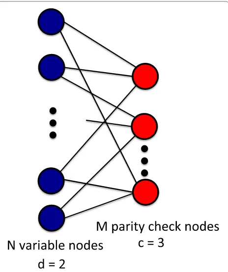
A matrixAcorresponds to a(s,)-expander graph with regular right degree d if and only if each column of A

has exactlyd“1”s, and for any set Sof right nodes with |S| ≤s, the set of neighborsN(S)of the left nodes has size N(S)≥(1−)d|S|. If it further holds that each row ofA

hasc“1”s, we sayAcorresponds to a(s,)-expander with regular right degreedand regular left degreec.

Assume [μ]i≥ 0 for all i. Let A ∈ RM×N be con-sisting of binary entries, which corresponds to a bipar-tite graph, illustrated in Fig. 4. We further consider a bipartite graph with regular left degreec (i.e., the num-ber of edges from each variable node is c) and regu-lar right degree d (i.e., the number of edges from each parity check node is d), as illustrated in Fig. 4. Hence, this requires Nc = Md. Expander graphs satisfy the above requirements. The existence of expander graphs is established in [40]:

Fig. 4Illustration of an expander graph withd=2 andc=3. Following coding theory terminology, we call the left variables nodes (there areNsuch variables), which correspond to the entries ofxt, and the right variables parity check nodes (there areMsuch nodes), which correspond to entries ofyt. In a bipartite graph, connections between the variable nodes are not allowed. The adjacency matrix of the bipartite graph corresponds to ourAorAt

Lemma 2([40])For any fixed >0andρM/N<1, when N is sufficiently large, there always exists an(αN,) expander with a regular right degree d and a regular left degree c for some constantsα∈(0, 1), d and c.

Theorem 5(Expander A)IfA corresponds to a(s, )-expander with regular degree d and regular left degree c, for any nonnegative vector[μ]i≥0, we have that

≥ M(1−) dN .

Hence, for expander graphs,is approximately greater thanM/N·(1/d), wheredis a small number.

4.4.4 Consequence

Combine the results above, we showed that for the regime where M and the signal strength are sufficiently large, the performance loss can be small (as indeed observed from our numerical examples). In this regime, when A

an expander graph), the ratio (31) EDD(N)/EDD(M) is lower bounded by(1/4)·d/(1−)for some small number >0, when Corollary1holds.

There is one intuitive explanation. Unlike in compressed sensing, where the goal is to recover a sparse signal and one needs the projection to preserve norm up to a fac-tor through the restricted isometry property (RIP) [41], our goal is to detect a non-zero vector in Gaussian noise, which is a much simpler task than compressed sensing. Hence, even though the projection reduces the norm of the vector, as long as the projection does not diminish the signal is normal below the noise floor.

On the other hand, when the signal is weak, andMis not large enough, there can be significant performance loss (as indeed observed in our numerical examples) and we cannot lower bound the relative performance measure. Fortunately, in this regime, we can use our theoretical results in Theorems 1 and 2 to design the number of sketchesMfor an anticipated worst-case signal strength , or determine the infeasibility of the problem, i.e., it is better not to use sketching since the signal is too weak.

5 Results: numerical examples

In this section, we present numerical examples to demon-strate the performance of the sketching procedure. We focus on comparing the sketching procedure with the GLR procedure without sketching (by letting A = I in the sketching procedure). We also compare the sketching procedures with a standard multivariate CUSUM using sketches.

In the subsequent examples, we select ARL to be 5000 to represent a low false detection rate (similar choice has been made in other sequential change-point detec-tion work such as [15]). In practice, however, the target ARL value depends on how frequent we can tolerate false detection (e.g., once a month or once a year). Below, EDDo

denotes the EDD whenA= I(i.e., no sketching is used). All simulated results are obtained from 104 repetitions. We also consider the minimum number of sketches

Mmin=arg min{M: EDD(M)≤δ+EDDo}, (35)

such that the corresponding sketching procedure is onlyδ sample slower than the full procedure. Below, we focus on the delay lossδ=1.

5.1 Fixed projection, Gaussian random matrix

First, consider GaussianA with N = 500 and different number of sketchesM<N.

5.1.1 EDD versus signal magnitude

Assume the post-change mean vector has entries with equal magnitude: [μ]i= μ0, to simplify our discussion.

Figure5a shows EDD versus an increasing signal magni-tudeμ0. Note that whenμ0andMare sufficiently large,

(a)

(b)

Fig. 5Abeing a fixed Gaussian random matrix: the standard deviation of each point is less than half of its value.aEDD versus_μ0,

when all [_μ]i=μ0;bEDD versuspwhen we randomly select 100p%

entries [_μ]ito be 1 and set the other entries to be 0; the smallest value ofpis 0.05

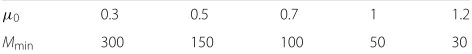
the sketching procedure can approach the performance of the procedure using the full data as predicted by our the-ory. When signal is weak, we have to use a much largerM to prevent a significant performance loss (and when sig-nal is too weak, we cannot use sketching). Table3shows Mminfor each signal strength; we find that whenμ0is

suf-ficiently large, we may even useMminless than 30 for an

Table 3AssumeAbeing a fixed Gaussian random matrix

μ0 0.3 0.5 0.7 1 1.2

Mmin 300 150 100 50 30

N = 500 to have little performance loss. Note that here, we do not require signals to be sparse.

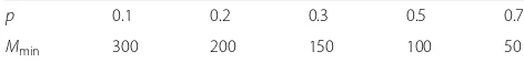
5.1.2 EDD versus signal sparsity

Now assume that the post-change mean vector is sparse: only 100p% entriesμibeing 1 and the other entries being 0. Figure5b shows EDD versus an increasingp. Note that as p increases, the signal strength also increases; thus, the sketching procedure will approach the performance using the full data. Similarly, theMminrequired is listed

in Table 4. For example, when p = 0.5, we find that one can use Mmin = 100 for an N = 500 with little

performance loss.

5.2 Fixed projection, expander graph

Now assumeAbeing an expander graph withN = 500 and different number of sketches M < N. We run the simulations with the same settings as those in Section5.1.

5.2.1 EDD versus signal magnitude

Assume the post-change mean vector [μ]i=μ0. Figure6a

shows EDD with an increasingμ0. Note that the simulated

EDDs are smaller than those for the Gaussian random projections in Fig.5. A possible reason is that the expander graph is better at aggregating the signals when [μ]i are all positive. However, when [μ]ican be either positive or negative, the two choices ofAhave similar performance, as shown in Fig.7, where [μ]i are drawn i.i.d. uniformly from [−3, 3].

5.2.2 EDD versus signal sparsity

Assume that the post-change mean vector has only 100p% entries [μ]i being 1 and the other entries being 0. Figure6b shows the simulated EDD versus an increasing p. Asptends to 1, the sketching procedure approaches the performance using the full data.

5.3 Time-varying projections with 0-1 matrices

To demonstrate the performance of the procedureT{0,1}

(21) using time-varying projection with 0-1 entries, again, we consider two cases: the post-change mean vector [μ]i= μ0and the post-change mean vector has 100p%

entries [μ]i being 1 and the other entries being 0. The simulated EDDs are shown in Fig.8. Note thatT{0,1}can

detect change quickly with a small subset of observations. Although EDDs ofT{0,1}are larger than those for the fixed

Table 4Abeing a fixed Gaussian random matrix

p 0.1 0.2 0.3 0.5 0.7

Mmin 300 200 150 100 50

MinimumMminrequired for various sparsity setting with parameterpas shown in Fig.5b.N=500,w=200, and 100p% of entries [μ]i=1

(a)

(b)

Fig. 6Abeing a fixed expander graph. The standard deviation of each point is less than half of its value.aEDD versusμ0, when all [μ]i=μ0; bEDD versuspwhen we randomly select 100p% entries [μ]ito be 1 and set the other entries to be 0; the smallest value ofpis 0.05

projections in Figs.5and6, this example shows that pro-jection with 0-1 entries can have little performance loss in some cases, and it is still a viable candidate since such projection means a simpler measurement scheme.

5.4 Comparison with multivariate CUSUM

Fig. 7Comparison of EDDs forAbeing a Gaussian random matrix versus an expander graph when [_μ]i’s are i.i.d. generated from [−3, 3]

settings, when all [μ]iare equal to a constant and when 100p% entries of the post-change mean vector are positive valued. In Fig.9, the log-GLR-based sketching procedure performs much better than the multivariate CUSUM.

6 Examples for real applications 6.1 Solar flare detection

We use our method to detect a solar flare in a video sequence from the Solar Data Observatory (SDO)1_{. Each} frame is of size 232 × 292 pixels, which results in an ambient dimensionN=67, 744. In this example, the nor-mal frames are slowly drifting background sun surfaces, and the anomaly is a much brighter transient solar flare emerges att = 223. Figure10a is a snapshot of the orig-inal SDO data att = 150 before the solar flare emerges, and Fig. 10b is a snapshot at t = 223 when the solar flare emerges as a brighter curve in the middle of the image. We preprocess the data by tracking and removing the slowly changing background with the MOUSSE algo-rithm [43] to obtain tracking residuals. The Gaussianity for the residuals, which corresponds to ourxt, is verified by the Kolmogorov-Smirnov test. For instance, thepvalue is 0.47 for the signal att = 150, which indicates that the Gaussianity is a reasonable assumption.

We apply the sketching procedure with fixed projection to the MOUSSE residuals, choosing the sketching matrix

Ato be anM-by-NGaussian random matrix with entries i.i.d. N(0, 1/N). Note that the signal is deterministic in this case. To evaluate our method, we run the procedure 500 times, each time using a different random Gaussian matrix as the fixed projectionA. Figure11shows the error bars of the EDDs from 500 runs. As Mincreases, both the means and standard deviations of the EDDs decrease.

1_{The video can be found at http://nislab.ee.duke.edu/MOUSSE/. The Solar}

Object Locator for the original data is SOL2011-04-30T21-45-49L061C108.

(a)

(b)

Fig. 8A_ts are time-varying projections. The standard deviation of each point is less than half of its value.aEDD versus_μ0, when all [μ]i=μ0; bEDD versuspwhen we randomly select 100p% entries [_μ]ito be 1 and set the other entries to be 0; the smallest value ofpis 0.05

WhenMis larger than 750, EDD is often less than 3, which means that our sketching detection procedure can reliably detect the solar flare with only 750 sketches. This is a sig-nificant reduction, and the dimensionality reduction ratio is 750/67, 744≈0.01.

6.2 Change-point detection for power systems

(a)

(b)

Fig. 9Comparison of the sketching procedure with a method adapted from multivariate CUSUM.aEDDs versus variousMs, when all [_μ]i=0.2;bEDDs versus variousMs, when we randomly select 10% entries [_μ]ito be 1 and set the other entries to be 0

Note that the graph is sparse and that there are many “communities” which correspond to densely connected subnetworks.

In this example, we simulate a situation for power fail-ure over this large network. Assume that at each time, we may observe the real power injection at an edge. When the power system is in a steady state, the observation is the true state plus Gaussian observation noise [45]. We may estimate the true state (e.g., using techniques in [45]), sub-tract it from the observation vector, and treat the residual vector as our signalxi, which can be assumed to be i.i.d. standard Gaussian. When a failure happens in a power system, there will be a shift in the mean for a small number of affected edges, since in practice, when there is a power failure, usually only a small part of the network is affected simultaneously.

To perform sketching, at each time, we randomly choose M nodes in the network and measure the sum of the quantities over all attached edges as shown in Fig. 13. This corresponds to A_ts with N = 6594 and various M < N. Note that in this case, our projection matrix is a 0-1 matrix whose structure is constrained by the net-work topology. Our example is a simplified model for power networks and aims to shed some light on the potential of our method applied to monitoring real power networks.

In the following experiment, we assume that on aver-age, 5% of the edges in the network increase byμ0. Set

the threshold b such that the ARL is 5000. Figure 14 shows the simulated EDD versus an increasing signal strength μ0. Note that the EDD from using a small

number of sketches is quite small if μ0 is sufficiently

large. For example, when μ0 = 4, one may detect

the change by observing from only M = 100 sketches (when the EDD is increased only by one sample), which is a significant dimensionality reduction with a ratio of 100/4941≈0.02.

(a)

(b)

Fig. 11Solar flare detection: EDD versus variousMwhenAis an M-by-NGaussian random matrix. The error bars are obtained from 104

repetitions with runs with different Gaussian random matrixA

7 Conclusion

In this paper, we studied the problem of sequential change-point detection when the observations are linear projections of the high-dimensional signals. The change-point causes anunknownshift in the mean of the signal, and one would like to detect such a change as quickly as possible. We presented new sketching procedures for fixed and time-varying projections, respectively. Sketch-ing is used to reduce the dimensionality of the signal and thus computational complexity; it also reduces data collection and transmission burdens for large systems.

Fig. 12Power network topology of the Western States Power Grid of the USA

Fig. 13Illustration of the measurement scheme for a power network. Suppose the physical quantities at edges (e.g., real power flow) at timeiform the vectorxi, we can observe the sum of the edge quantities at each node. When there is a power failure, some edges are affected, and their means are shifted

The sketching procedures were derived based on the generalized likelihood ratio statistic. We analyzed the theoretical performance of our procedures by deriving approximations to the average run length (ARL) when there is no change, and the expected detection delay (EDD) when there is a change. Our approximations were shown to be highly accurate numerically and were used to understand the effect of sketching.

We also characterized the relative performance of the sketching procedure compared to that without sketching. We specifically studied the relative performance mea-sure for fixed Gaussian random projections and expander graph projections. Our analysis and numerical examples

Fig. 14Power system example:Abeing a power network topology constrained sensing matrix. The standard deviation of each point is less than half of the value. EDD versusμ0when we randomly select

showed that the performance loss due to sketching could be quite small in a big regime when the signal strength and the dimension of sketches Mare sufficiently large. Our result can also be used to find the minimum requiredM given a worst-case signal and a target ARL. In other words, we can determine the region where sketching results in little performance loss. We demonstrate the good per-formance of our procedure using numerical simulations and two real-world examples for solar flare detection and failure detection in power networks.

On a high level, although after sketching, the Kullback-Leibler (K-L) divergence becomes smaller, thethreshold b for the same ARL also becomes smaller. For instance, for Gaussian matrix, the reduction in K-L divergence is compensated by the reduction of the thresholdbfor the same ARL, because the factor that they are reduced by are roughly the same. This leads to the somewhat counter-intuitive result that the EDDs with and without sketching turns to be similar in this big regime.

Thus far, we have assumed that the data streams are independent. In practice, if the data streams are depen-dent on aknowncovariance matrix, we can whiten the data streams by applying a linear transformation−1/2xt. Otherwise, the covariance matrixcan also be estimated using a training stage via regularized maximum likelihood methods (see [46] for an overview). Alternatively, we may estimate the covariance matrix of the sketchesAA

orAtAt directly, which requires fewer samples to esti-mate due to the lower dimensionality of the covariance matrix. Then, we can build statistical change-point detec-tion procedures using(similar to what has been done for the projection Hotelling control chart in [19]), which we leave for future work. Another direction of future work is to accelerate the computation of sketching using techniques such as those in [47].

Appendix 1: Proofs

We start by deriving the ARL and EDD for the sketching procedure.

Proofs for Theorems1and2This analysis demonstrates that the sketching procedure corresponds to the so-called mixture procedure (cf. T2 in [15]) in a special case of p0 = 1,Msensors, and the post-change mean vector is Vμ. In [15], Theorem 1, it was shown that the ARL of the mixture procedure with parameterp0 ∈[ 0, 1] andM

sensors is given by

E∞_{{T} ∼H(M,θ}

where the detection statistic will search within a time win-dowm0≤t−k≤m1. Letg(x,p0)=log(1−p0+p0ex

Note thatU2isχ₁2distributed, whose MGF is given by

EeθU2=1/√1−2θ. Hence, whenp0=1,

The first-order and second-order derivative of the log MGF are given by, respectively,

˙

Combining the above, we have that the ARL of the sketching procedure is given by

E∞_{{T} =} θ0

the two terms in the above expression can be written as

then (39) becomes

Finally, note that we can also write

γ (θ0)=θ02/[ 2(1−θ0)]=(1−M/(2b))2/(M/b),

and the constant is

c(M,b,w)=

We are done deriving the ARL. The EDD can be derived by applying Theorem 2 of [15] in the case where = Vμ, the number of sensors isM, andp0=1.

The following proof is for the Gaussian random matrixA.

Proof of Theorem4 It follows from (32), and a standard result concerning the distribution function of the beta distribution ([48], 26.5.3) that

P{≤b} =Ib

whereIis the regularized incomplete beta function (RIBF) ([48], 6.6.2). We first prove the lower bound in (34). AssumingN→ ∞such that (33) holds, we may combine (41) with ([49], Theorem 4.18) to obtain

lim

from which it follows that there existsN˜ such that for all N≥ ˜N,

1

N lnP{ ≤δ−}<− c 2, which rearranges to give

P{≤δ−}<e−c

N

2 _,

which proves the lower bound in (34). To prove the upper bound, it follows from (41) and a standard property of the RIBF ([48], 6.6.3) that

P{≥b} =I1−b

combine (42) with ([49], Theorem 4.18) to obtain

lim

and the argument now proceeds analogously to that for the lower bound.

Lemma 3If a 0-1 matrixAhas constant column sum d, for every non-negative vectorxsuch that[x]i≥0, we have (s,)-expander with regular degree d and regular left degree c, for any nonnegative vectorx,

Ax2

Proof of Lemma4For any nonnegative vectorx,

= holds for exactlyd rows. And for each rowi of these d rows,Ail = 1 for exactly ccolumns withl ∈ {1,. . .,p}; (47) holds sincedN = Mc. Finally, from the definition of σmax, (45) holds.

Proof for Theorem5 Note that

= (μV Vμ)1/2=(muAU−2UAμ)1/2

≥ σ−1

max(A)UAμ2=σmax−1(A)Aμ2, (48)

whereσmax=σmax(A), and (48) holds sinceUis a unitary

matrix. Thus, in order to bound, we need to charac-terize σmax, as well as Aμ2 for a s sparse vector μ.

Combining (48) with Lemma3 and 4, we have that for every nonnegative vectorμ, [μ]i≥0,

Finally, Lemma 2 characterizes the quantity [M(1 − )/(dN)]1/2_{in (49) and establishes the existence of such}

an expander graph. WhenA corresponds to an (αN,) expander described in Lemma2,≥ βμ2for all

non-negative signals [μ]i≥ 0 for some constantα and some constantβ=(ρ(1−)/d)1/2. Done.

Proof for Corollary1 We define that x M/b, then Theorem1tells us that whenMgoes to infinity, we have that that (50) holds. Next, we prove the claim.

Define the logarithm of the right-hand side of (50) as follows:

integration, we know that,₀∞uν2(u)du < 1. Therefore, −log(C(M,x,w)) >0. Then,

We define that x0 is the solution to the following

equation:

Then, we have that

C(M,x0,w) >

where the second inequality is due to the fact that the upper bound for the integral interval is 1 and the third inequality is due to the fact that exp(−x) is a convex function. Therefore, we have that