R E S E A R C H
Open Access
Sequential convex combinations of
multiple adaptive lattice filters in cognitive
radio channel identification
Mehmet Tahir Ozden
Abstract
Sequential convex combinations of multiple adaptive lattice filters using different exponential weighting factors in cognitive radio (CR) channel identification framework have been considered in this presentation. First, the sequential processing multichannel lattice stages (SPMLSs) are modified so as to be used in filter combination task. Then, two different combination schemes, i.e., regular combination of multiple lattice filters (R-CMLF) and decoupled
combination of multiple lattice filters (D-CMLF), that utilize modified SPMLSs as filter structure have been proposed. A modified Gram-Schmidt orthogonalization of multiple channels of data, which is constituted in multiple filter combination task, is accomplished. A highly modular, regular, and reconfigurable filter structure, which is suitable for cognitive radios, is achieved with the combination processing implemented in an order-recursive fashion. The mean square deviation (MSD) performances of the schemes under stationary and nonstationary conditions have been presented and compared with the performances of multiple combination of least mean square (M-CLMS), decoupled combination of least mean square (D-CLMS) schemes, and component filters. It has also been shown that the fault tolerances of the proposed schemes are better than those of the component filters due to the redundancy
introduced with combination processing, and that the proposed schemes bring together the desired adaptive filter features such as fast convergence and low steady-state MSD levels, which do not normally coexist.
Keywords: Cognitive radio, CR, 5G, Combining filters, Channel identification, Lattice filters, Sequential processing
1 Introduction
Cognitive radio (CR) and 5G are two recent developments in the design of next-generation wireless communica-tion systems. CR is built on a software radio, funccommunica-tions as an intelligent system that is aware of its environment and uses the methodology of understanding-by-building to learn from the environment, and adapts to statistical variations in the input stimuli in order to establish reli-able communication by efficient utilization of the radio spectrum [1–4].
A typical CR cycle includes spectrum sensing, analy-sis, reasoning, and adaptation to new operating parameter steps [5]. CR can detect the availability of a portion of frequency band through spectrum sensing and analysis steps [6]. During the reasoning step, it determines the
Correspondence:[email protected]
Piri Reis University, Faculty of Engineering, Department of Electrical and Electronics Engineering, Tuzla, 34940 Istanbul, Turkey
optimum operating parameters, so that no harmful inter-ference to other users of the spectrum is generated due to its transmission. In the adaptation step, the radio switches to transmission and reception mode using its reconfig-urability and reprogrammability property [7,8], and tunes its operating parameters according to its best response strategy.
The concept of software radio as the backbone of CR on the other hand relies on the development of DSP technol-ogy that is flexible, reconfigurable, and reprogrammable by software to adapt to an environment where there are multiple services, standards, and frequency bands [8–11]. Correspondingly, the infrastructure in a software radio system is generally required to use reconfigurable VLSI hardware components such as DSP chip sets [12], FPGAs [13], embedded processors [14], and even general purpose processors [15].
An emerging requirement for CRs is location and envi-ronment awareness that involves modeling the capabilities
of human beings and bats for realization of advanced and autonomous location and environment awareness features [16, 17]. Adaptive positioning, determining the coordinates of a cognitive radio in space, is a step towards realization of accurate location awareness in cognitive radios [18]. The author has recently proposed a receiver (equalizer) architecture for use in cognitive MIMO-OFDM radios that performs joint channel estimation and data detection, addresses the receiver complexity prob-lems, and contributes to the flexibility, reconfigurability, and reprogrammability of receiver [19]. It was also shown in [20–22] that this receiver architecture can be config-ured for spectrum sensing as well as adaptive positioning function of cognitive radio virtually at no cost.
In parallel with the developments in CR, 5G has been introduced connoting features such as increased data rates, spectral efficiency, and low latency through extreme densification, massive MIMO, device-centric architec-tures, millimeter wave, smarter devices, native support for machine-to-machine (M2M) communication, and inter-ference management [23,24]. As the future mobile broad-band will be largely driven by ultra-high-definition video and as the things around us will be always connected, it is envisioned that the new era of communication will be dominated by the need for more capacity as well as spec-trum, which will result in the integration of cognitive radio concepts in 5G networks [25,26].
Another important concept that can find application in CRs is related to combining of adaptive filters [27]. When a priori knowledge about the filtering scenario is limited or imprecise, as in a typical cognitive radio oper-ational cycle [1], implementing the most adequate filter structure and adjusting its parameters becomes a difficult task, and inaccurate choices may result in poor perfor-mance. An intelligent way to overcome this difficulty is to rely on combining of adaptive filters, in an attempt to improve their properties in terms of convergence, tracking ability, steady-state misadjustment, robustness, or compu-tational cost. Combining adaptive filters can also improve reliability by introducing redundant processing elements, i.e., by stepping up the natural fault tolerance inherent in adaptive filters. Note that the notion of improving relia-bility by introducing redundancy is in line with the recent developments in the field of reliable control, particularly, with the application of a system augmentation approach that reformulates the original system into a descrip-tor piecewise affine system and then takes advantage of the redundancy of this descriptor system formulation [28,29], and that the concept of adaptivity itself can be considered as a form of intelligence built into a filtering mechanism.
It is possible to combine adaptive filters implementing different tasks or using different filter operating parame-ters, structures, and learning algorithms [30]. The recent
examples of adaptive filter combination tasks include the combination of adaptive filters from different families such as one gradient and one Hessian based in [31], the adaptive combination of proportionate filters for sparse echo cancelation in [32], the adaptive combination of subband adaptive filters for acoustic echo cancelation in [33], the convex combination of H2 and H∞ filters for space-time adaptive equalization in [34], the online track-ing of the changes in the nonlinearity within a signal by using a collaborative adaptive signal processing approach based on a combination (hybrid) filter in [35], the adap-tive combination of Volterra kernels and its application to nonlinear echo cancelation in [36], the convex combina-tion of nonlinear adaptive filters for active noise control in [37], the combination of adaptive filters for relative navigation in [38], finite impulse response (FIR)-infinite impulse response (IIR) adaptive hybrid combination in [39], the affine combination of two adaptive sparse filters for estimating large-scale multiple-input multiple-output (MIMO) channels in [40], the combinations of multiple kernel adaptive filters in [41], the low-complexity approx-imation to the Kalman filter using convex combinations of adaptive filters from different families in [42], and the proposition of a family of combined-step-size proportion-ate filters in [43].
Two possible strategies for combining filters are con-vex and affine combinations, where the mixing coefficient is restricted to be nonnegative and sum up to one and the condition on the mixing parameter is relaxed, allow-ing it to be negative respectively [44–46]. In fact, the affine combination scheme can be interpreted as a gen-eralization of the convex combination since the mixing coefficient is not restricted to the interval [0,1]. Even though the affine combination scheme allows for smaller error levels in theory, it suffers from larger gradient noise in some situations [47]. The adaptation rule for the mixing coefficient in affine combinations is simpler than those in convex ones, and the correct adjustment of the step size for the updating of the mixing coefficient depends on some characteristics of the filtering scenario. Accordingly, the desired universal behavior for the affine combination, in which case the combined estimate is at least as good as the best of the component filters in steady state, cannot always be ensured, whereas convex combinations have a built-in mechanism to attain such universality [47].
combination schemes. In order to capture the statistical variations in the CR environment, the combination of multiple lattice filters with different exponential weight-ing factors has been considered so as to brweight-ing together the convergence properties of fast filters that have small expo-nential weighting factors and steady-state MSD properties of slow filters that have large exponential weighting fac-tors. Accordingly, the author envisions multiple adaptive lattice filters as channels of sequential processing multi-channel lattice stages (SPMLSs) [19–22,50] and proposes to sequentially combine these multiple lattice filters in a CR channel identification task. In view of the aforemen-tioned issues concerning convex vs. affine combinations, the focus is on convex combinations of multiple adaptive lattice filters.
As the first contribution, the regular combination of multiple transversal filters in [49] is adapted to multiple lattice filters, and then, as the second contribution, the decoupled combination of two transversal filters in [49] is extended to multiple filters and tailored to multiple lattice filters by developing order-recursive algorithms for com-bination processing and also by making use of orthogo-nalized data and multichannel lattice filter parameters. To the best of the author’s knowledge, neither schemes exist in the literature. Note that a complete modified Gram-Schmidt orthogonalization of multichannel input data, which avoids matrix inversions and enables scalar only operations, is attained, and this feature is considered criti-cal, as matrix inversion is a major bottleneck in the design of embedded receiver architectures [51]. Additionally, the computational complexity as well as the performances of the proposed lattice filter combination schemes in station-ary and nonstationstation-ary channel identification scenarios are investigated and compared to those of the multiple com-bination of least mean square (M-CLMS) and decoupled combination of least mean square (D-CLMS) schemes in [49].
The organization of this paper is as follows. Section2 is about the problem formulation in which channel model and multiple channel identification are introduced. In Section3, the original SPMLS is initially introduced, and then, the proposed modifications in the SPMLS are dis-cussed. Subsequently, the regular combination of multiple lattice filters (R-CMLF) and decoupled combination of multiple lattice filters (D-CMLF) schemes are presented in Sections4and5respectively. The experimental results are accounted for in Section 6, and finally, Section 7 is concerned with conclusions.(•)∗represents the complex conjugate of(•).(•)Tand(•)Hstand for the transpose and the Hermitan transpose of(•)respectively. The variablesi andnare the time indexes related to data and coefficients respectively,mis the index for the number of combining filters, and finally,stands for the stage number of lattice filters.
2 Problem formulation
2.1 Channel model
The cognitive radio channel is modeled by using the tapped delay line model [52,53], and the channel output signal,y(i), in this model is given by :
y(i)=wH(n)x(i)+u(i), i=1, 2,. . .,n, (1)
where x(i)=[x(i),x(i−1),. . .,x(i −N+ 1)]T refers to the input signal vector.u(i)is the channel noise signal at time instantiand is a realization of white, independently and identically distributed (i.i.d.) Gaussian random pro-cess with zero mean and constant varianceσ2
u and is also independent ofx(i).
Herein, w(n)=[w0(n),w1(n),. . .,wN−1(n)]T is the channel coefficient vector defined over the entire obser-vation interval 1 ≤ i ≤ n, andN is the channel length. The channel coefficient vector in the model is assumed to change in accordance with the first-order Markov process in [54]:
w(n+1)=a.w(n)+q(n), (2)
whereq(n)represents an i.d.d. Gaussian-distributed ran-dom zero-mean vector with diagonal covariance matrix Q(n) = Eq(n)qH(n). Herein, E[•] is defined as the statistical expectation operator. The initial values of the coefficient vector, wH(−1), are also assumed Gaus-sian distributed with zero mean and variance σ2
w and independent of q(n), u(i), and x(i). a is a constant close to 1.
For the channel defined by Eqs. (1) and (2), the degree of nonstationarity is stated in [54,55] as:
ξ(n)= E
|qH(n)x(n)|2
E[|u(n)|2] . (3) For slow statistical variations,ξ(n)is small, and typically less than unity, whereas it is greater than unity for fast sta-tistical variations, indicating that it is not advantageous to build an adaptive filter to solve the tracking problem.
2.2 Multiple channel identification
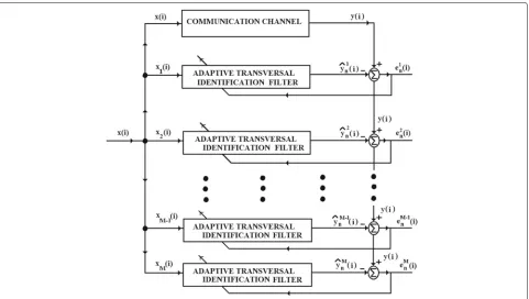
Figure1depicts the multiple channel identification prob-lem under consideration, in which information about the channel and scenario is assumed available through CR’s network, or through CR’s analysis, reasoning, and adapta-tion cycles. The objective in this problem is to estimate the coefficients of channel in (1) using multiple exponentially weighted least squares (LS) adaptive filters, each of which is implemented with a different exponential weight factor. Accordingly, the optimal exponentially weighted LS solu-tion for the coefficients of themth filter can be found by minimizing the following cost function:
Fig. 1A diagram of the multiple channel identification problem
at time instantn, wherem= 1, 2,. . .,Mand is the index for the component filters, and the use of prewindowing is assumed.λmis the exponential weighting factor for the mth filter. δ is a positive real number called the regu-larization parameter [56]. Herein, the coefficient vector of the mth adaptive filter, Pm(n), at time instant n, is delineated as:
Pm(n)=[Pm,0(n),Pm,1(n),. . .,Pm,Nm−1(n)]T, (5)
and its 2− norm is defined as Pm(n)2 = Nm−1
k=0 Pm,k(n)2 1/2
. Themth estimation error at time instanti, computed using the input signal at time instanti and the filter coefficients at time instantn, is given by :
emn(i)=y(i)−PHm(n)xm(i), i=1, 2,. . .,n, (6)
where the input signal vector to the mth adaptive filter, xm(i), at time instanti, is defined as :
xm(i)=[xm(i),xm(i−1),. . .,xm(i−Nm+1)]T. (7)
Note thatxm(i)= x(i),∀m,Nmis the length of themth filter.
Subsequently, the mth optimal coefficient vector is found by differentiatingJm(n)with respect toPm(n), set-ting the derivative to zero, and solving forPm(n):
Poptm (n)=Rxmxm−1 (n)Rxmy(n), (8)
whereRxmxm(n)is theNm×Nmcorrelation matrix ofxm(i) and is given by :
Rxmxm(n)= n
i=1 λn−i
m xm(i)xHm(i)+ δλnmI, (9)
in which the appearance of the second summational term is due to the regularizing term δ λn
m Pm(n)22 in the cost functionJm(n), andIis Nm× Nm identity matrix. TheNm×1 cross-correlation matrix ofxm(i)andy(i)is expressed as:
Rxmy(n)=
n
i=1 λn−i
m xm(i)y∗(i). (10)
Note that the channel length information can be avail-able through the implementation of a channel length estimation algorithm such as [57] in CR. Accordingly, the lengths of all adaptive filters are assumed equal to the length of the channel to be identified, that is,Nm=N. All prediction and estimation errors hereafter are shown for the end of the observation intervali=n.
3 Sequential multichannel lattice processing
updating of a priori reflection coefficient form of process-ing equations in [58,59] respectively. We then introduce the modifications to be implemented in the SPMLS in order to be able use its channels as filters in a combination task.
3.1 The original SPMLS
The original SPMLS has a block structure as shown in Fig. 2, and the input signal vectors to the SPMLS are defined as follows : the input forward prediction error vector,
f−1(n)= f0−1(n),f1−1(n),. . .,. . .,fM−−11(n),fM−1(n) T
,
(11)
the backward prediction error vector,
b−1(n)= b0−1(n),b1−1(n),. . .,. . .,bM−−11(n),bM−1(n) T
,
(12)
and the estimation error vector,
e−1(n)= e0−1(n),e1−1(n),. . .,. . .,eM−−11(n),eM−1(n) T
.
(13)
The elements of input forward and backward predic-tion error vectors in Eqs. (11) and (12) are orthogonalized by using self-orthogonalization processors (SOPs), which are triangular-shaped processors in Fig.2. The outputs of SOPs are given in the orthogonalized forward prediction error vector,
ˆ
f−1(n)= fˆ0−1(n),fˆ1−1(n),. . .,. . .,fˆM−−11(n),fˆM−1(n) T
(14)
and the orthogonalized backward prediction error vector,
ˆ
b−1(n)= bˆ0−1(n),bˆ1−1(n),. . .,. . .,bˆM−−11(n),bˆM−1(n) T
.
(15)
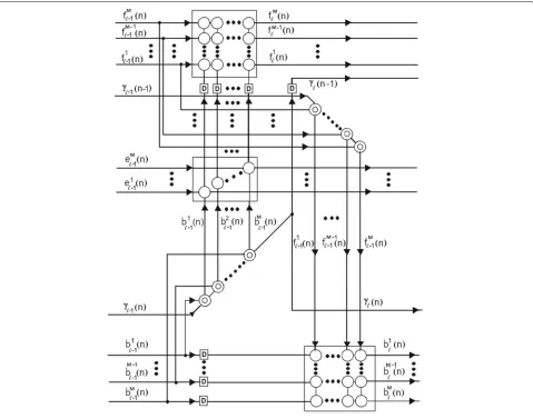
Fig. 3A diagram of the modified SPMLS
The elements of fˆ−1(n) are fed into a forward pre-diction reference-orthogonalization processor (ROP) in order to predict the elements ofb−1(n−1)and to pro-duce the stage output back prediction error vectorb(n). The elements of bˆ −1(n) are similarly fed into a ROP to perform M-channel joint process estimation and to produce the stage output estimation error vector e(n). Subsequently, the elements of bˆ−1(n) are delayed and are also fed into another ROP to obtain the stage output forward prediction error vectorf(n).
There are two types of processing cells, single and double circular processors in a SPMLS, and the com-plete SPMLS algorithm, which includes the processing equations in these cells, is provided in Table1.
3.2 Modification of the SPMLS
In combining multiple filters, we take into account that input signals to all combining filters are the same as indicated in the sentence right after (7) and modify
the SPMLS by removing all single circular cells in self-orthogonalizing processors and redundant single circular cells in referential-orthogonalizing processors. Accord-ingly, the modified SPMLS does not have the orthogonal-ized forward and backward prediction errors that consti-tute the vectors in Eqs. (14) and (15). It neither includes the cross-estimation error terms in the ROP related to the joint-process estimation. The modified SPMLS and its algorithm are presented in Fig.3and Table2respectively.
4 Combinations of multiple lattice filters
Table 1The original SPMLS algorithm
they are computed locally in the D-CMLF scheme and therefore stage dependent. Hence, the total number of combination parameters and mixing coefficients in the R-CMLF and D-R-CMLF schemes isMandM×Nrespectively.
4.1 Regular combination of multiple lattice filters A diagram of the R-CMLF scheme for M = 2 case, that is, the regular combination of two lattice filters (R-CTLF), is presented in Fig.4. Two types of combination
processors are introduced into the filter structure in this scheme: a type-1 combination processor per stage and a type-2 processor to the final stage. In the following, we present the development of combination algorithms that will be implemented by type-1 and type-2 processors in the R-CMLF scheme.
Table 2The modified SPMLS algorithm cient and thekth estimation error reflection coefficient of thejth lattice stage at time instantnrespectively.bkj−1(n) is the kth backward prediction error at the entrance of the jth stage at time instant n. The estimate of equiva-lent desired signal can be expressed order-recursively as follows :
ˆ
deq,n(n)= ˆdeq−1,n(n)+vm(n) ∗,m(n−1)bm−1(n), (17)
where=1,. . .,N,m=1,. . .,M, anddˆq0,n(n)=0. Then, Eq. (17) is substituted in:
eeq,n(n)=d(n)− ˆdeq,n(n), (18)
to obtain the following expression:
eeq,n(n)=d(n)− ˆdeq−1,n(n)−vm(n) ∗,m(n−1)bm−1(n). (19)
Herein,d(n)represents the desired signal at time instant n, which is the channel output signal y(n) in the chan-nel identification problem. Subsequently, the equivalent estimation error at the(−1)th stage is defined as:
eeq−1,n(n)=d(n)− ˆdeq−1,n(n), (20)
in order to achieve the order-recursive expression for the equivalent estimation error as:
eeq,n(n)=eeq−1,n(n)−vm(n) ∗,m(n−1)bm−1(n). (21)
It can be similarly shown that the equivalent estima-tion error,eeq,n(n), at the output of theth stage can also be expressed in terms of estimation errors related to the channels of SPMLSs as: The corresponding equivalent reflection coefficient at the th stage can be computed using mixing and reflection coefficients at time instantnas:
eq
Fig. 4A diagram of the R-CTLF scheme
Themth mixing coefficient at time instantn+1 is com-puted at the output of the last lattice stage in a type-2 combination processor as follows:
vm(n+1)= exp(a
m(n+1))
β(n+1) , (24)
wherem = 1, 2,. . .,M, andam(n+1)is themth com-bination parameter at time instant n + 1. Herein, the normalization parameter at time instantn+1,β(n+1), is computed according to:
β(n+1)= M
k=1
exp
ak(n+1)
. (25)
Note that 0<vm(n) <1,∀m, andMk=1vk(n)=1. The time-update equation for the mth combination parameter,am(n), can be accordingly expressed as:
am(n+1)=am(n)−μa 2
∂eeqN,n(n)2
∂am(n) , (26)
in which μa is the step size. The derivation in (26) is carried out so as to obtain the following expression:
am(n+1)=am(n)−μaeeqN,n(n)∂e
eq N,n(n)
∂am(n) . (27) Equation (22) for=Nis subsequently utilized in
eval-uating∂e eq N,n(n)
∂am(n), and Eq. (27) is expressed as in the following statement:
am(n+1)=am(n)−μaeeqN,n(n)
M
k=1 ∂vk(n)
∂am(n) e k N,n(n),
(28)
wherem=1,. . .,M. The partial derivatives ofvk(n)with respect toam(n)are stated as follows:
∂vm(n) ∂am(n) =v
m(n)−vm(n)2, k=m
∂vk(n)
∂am(n) = −v
k(n)vm(n), k=m.
(29)
in Eq. (28) to attain the following statement for the time-update equation of themth combination parameter:
am(n+1)= am(n)−μaeeqN,n(n) find an equivalent expression for the summation term,
k=m
vk(n)ekN,n(n), in Eq. (30) as follows:
eeqN,n(n)−emN,n(n)=
k=m
vk(n)ekN,n(n), (31)
which is then substituted back in Eq. (30), and the final expression for the time-update of the mth combination parameter in terms of the indexmis attained as:
am(n+1)=am(n)−μaeeqN,n(n)emN,n(n)−eeqN,n(n)vm(n), (32)
where m = 1,. . .,M. The term emN,n(n)−eeqN,n(n) in Eq. (32) can give rise to a slowing down effect in the learn-ing of combination parameters that usually occurs dur-ing long stationary intervals durdur-ing which the estimation errors,emN,n(n)andeeqN,n(n), are close. In order to alleviate this problem, a momentum term can be appended to the statement in Eq. (32) as in the following :
am(n+1) = am(n)−μaeeqN,n(n)
emN,n(n)−eeqN,n(n)vm(n) +ρ(am(n)−am(n−1)), (33) where 0< ρ <1 [49]. Accordingly, the new additive term in Eq. (33) compensates the pernicious effect related to the second term.
The mixing coefficients, vm(n), are then fed back to type-1 combination processors so as to be used in the computation of equivalent desired signals, estimation errors, and equivalent reflection coefficients in Eqs. (17), (21), or (22) and (23) respectively. We call the complete algorithm as the R-CMLF algorithm, which includes the modified SPMLS algorithm in Table 2 as well as the combination algorithm presented in this subsection, and summarize it in Table3.
It is also possible to speed up the convergence of the slower component filters by transferring a part of the equivalent reflection coefficients to the reflection coeffi-cients of the component filters that perform significantly worse than the combined scheme. To accomplish this objective, Eq. (T.3.9) in Table 3 regarding the computa-tion of the mth joint state estimation lattice reflection coefficient at the th stage is modified by incorporating the transfer parameter α and the equivalent reflection
coefficient eq (n−1) at theth stage in the following The permissible range for the transfer parameter is 0< α < 1, and the transfer of reflection coefficients is only applied when the filtered quadratic estimation errors meet the conditions discussed in [49] as indicators of worse performance.
4.2 Decoupled combination of multiple lattice filters A diagram of the D-CMLF scheme is presented forM=2 case, which can be named as decoupled combination of two lattice filters (D-CTLF), in Fig.5. A type-3 combina-tion processor in this case is inserted to each lattice stage. In the sequel, we develop the combination algorithm that will be implemented in a type-3 processor.
In order to compute the estimate of equivalent desired signal at the output of theth lattice stage in an order-recursive manner, it is first stated as follows:
ˆ error reflection coefficients of thejth lattice stage at time instantnrespectively.bkj−1(n)is thekth backward predic-tion error at the entrance of thejth stage at time instanti. The estimate of equivalent desired signal can be expressed order-recursively as follows :
ˆ
deq,n(n)= ˆdeq−1,n(n)+vm(n) ∗,m(n−1)bm−1(n), (36)
for=1,. . .,N,m=1,. . .,M, anddˆeq0,n(n)=0. Note the mixing coefficients are related to theth stage in this case. Subsequently, the equivalent estimation error at the output of theth stage is defined as :
eeq,n(n)=d(n)− ˆdeq,n(n), (37)
whered(n)represents the desired signal at time instantn as in the previous subsection, and Eq. (36) is substituted in this equivalent estimation error expression to obtain the following statement:
eeq,n(n)=d(n)− ˆdeq−1,n(n)−vm(n) ∗,m(n−1)bm−1(n). (38)
The equivalent estimation error for the(−1)th stage is similarly defined as :
eeq−1,n(n)=d(n)− ˆdeq−1,n(n), (39)
and thereby the order-recursive equivalent estimation error is expressed as:
Table 3The R-CMLF algorithm It can be shown that the equivalent estimation error,
eeq,n(n), at the output of theth stage can also be expressed in terms of estimation errors related to the channels of SPMLSs as: Similarly, the equivalent reflection coefficient at theth stage is stated in accordance with :
eq
Fig. 5A diagram of the D-CTLF scheme
n+ 1 for the th stage respectively. The normalization factor is defined as:
β(n+1)= M
k=1
exp
ak(n+1)
. (44)
Note that 0<vm(n) <1,∀mand, andMk=1vk(n)=1. It follows that the time-update equation for the mth combination parameter at the th stage, am(n), can be stated by making use of the gradient descent method as:
am(n+1) = am(n)−μa 2
∂eeq,n(n)2
∂am(n) , (45)
in which μa is the step size. The derivation in (45) is carried out so as to obtain the following expression:
am
(n+1) = am(n)−μaeeq,n(n) ∂eeq,n(n)
∂am
(n). (46)
Equation (41) is subsequently utilized in evaluating ∂eeq,n(n)
∂am(n), and Eq. (46) is expressed as in the following state-ment:
am(n+1)=am(n)−μaeeq,n(n)
M
k=1 ∂vk(n)
∂am(n)e
k ,n(n),
(47)
wherem=1,. . .,Mand=1,. . .,N. The partial deriva-tives ofvk(n)with respect toam(n)are found as follows:
∂vm(n)
∂am(n) = vm(n)−vm(n)2, k=m ∂vk
(n)
∂am
(n) = −v
k
(n)vm(n), k=m.
(48)
in Eq. (47) to obtain the following statement for the time-update equation of themth combination parameter at the th stage:
Afterwards, Eq. (41) is used to find an equivalent expres-sion for the summation term,
k=m
which is again used in Eq. (49) and the redundant term, and the final expression for the time-update of themth combination parameter at the th stage in terms of the indicesmandis given as:
am(n+1)=am(n)−μaeeq,n(n) (em,n(n)−eeq,n(n))vm(n), (51)
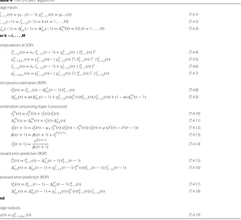
where = 1,. . .,Nandm = 1,. . .,M. Accordingly, the D-CMLF algorithm is presented in Table4.
Table 4The D-CMLF algorithm
In order to avoid the slowing down of learning effect in long stationary intervals, the modification of the time-update equation can be carried out by adding a momen-tum term to the statement in Eq. (51) as in:
am(n+1)=am(n)−μaeeq,n(n) (em,n(n)−eeq,n(n)) ×vm(n) + ρ(am(n)−am(n−1)), (52) where 0< ρ < 1 as before. To speed up the convergence of the slower component filters, Eq. (T.4.9) in Table 4, which is related to the computation of themth joint state estimation lattice reflection coefficient at theth stage, is modified as in Eq. (34).
5 Computational complexity
The computational complexity of the proposed schemes can be accordingly calculated by taking into consideration the effect of modifications on the complexity of a SPMLS and the added complexity due to combination processing in Eqs. (22) or (23), (24) and (25), and (32) in the R-CMLF scheme and Eqs. (41) or (42), (43) and (44), and (51) in the D-CMLF scheme. Note that computational complex-ity is expressed in terms of number of required operations, where one operation is considered as one multiplication (division) and one addition.
Due to the removal of all single circular cells in self-orthogonalizing processors and redundant single circular cells in referential-orthogonalizing processors of a SPMLS in combining multiple lattice filters, the complexity of a SPMLS reduces from (12M2 +7M) to (12M2 +M). Therefore, the total complexity for the R-CMLF scheme is(12NM2+2MN +3M+1), whereas it is(12NM2+ 5MN+N)for the D-CMLF scheme. If the convergence of the slower component filters is required to be sped up by transferring a part of the equivalent reflection coefficients to the reflection coefficients of the component filters, the complexities of the proposed schemes increase due to
the transfer term in Eq. (34), and momentum terms in Eqs. (33) and (52), which together amount to an additional complexity of(2MN+5M−N+3). Accordingly, the total complexities for the R-CMLF and D-CMLF schemes with transfer and momentum (t/m) terms become(12NM2+ 4MN +8M−N+4) and(12NM2+7MN +5M+3) respectively.
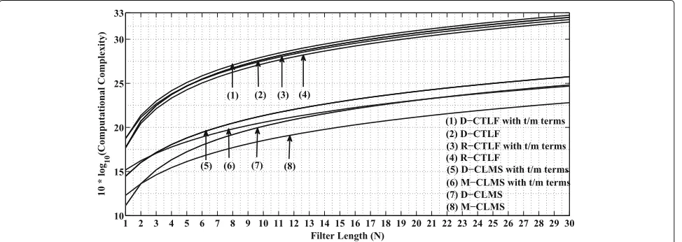
The computational complexities vs. filter length(N) curves of the R-CMLF and D-CMLF schemes forM=2, 4, and 8 cases, that is, R-CTLF, R-CTLF with t/m terms, D-CTLF, D-CTLF with t/m terms, regular combination of four lattice filters (R-CFLF), R-CFLF with t/m terms, decoupled combination of four lattice filters (D-CFLF), D-CTLF with t/m terms, regular combination of eight lat-tice filters (R-CELF), R-CELF with t/m terms, decoupled combination of eight lattice filters (D-CELF), and D-CELF with t/m terms have been plotted in Figs. 6, 7, and 8 respectively.
We have also compared the complexities of the pro-posed methods with those of M-CLMS whenM=2, 4, 8, and D-CLMS schemes in [49]. Note that the complexities of M-CLMS and D-CLMS schemes are 3MN +5M+1 and 10N+3 respectively and that these complexities also increase by an amount of 2MN + 5M − N + 3 when the transfer and momentum terms are implemented. In these figures, it can be seen that the complexities of the M-CLMS and D-CLMS schemes are advantageous com-paring to the R-CMLF and D-CMLF schemes mainly due to the well known simplicity of LMS filters, and this advantage becomes larger with increasing number of combining filters (M). However, it can be also noted that the complexities of transfer and momentum terms are comparable to those of the core M-CLMS and D-CLMS schemes, and therefore, the addition of transfer and momentum terms influences the complexities of M-CLMS and D-M-CLMS schemes more noticeably.
Fig. 7Computational complexity comparison forM=4
In Fig. 9, the complexities of the proposed schemes with different values of combining filters are compared. It can be noticed that there is slight difference between the complexities of the R-CMLF and D-CMLF schemes, and this difference disappears with increasing M. For N = 30, the R-CTLF and D-CTLF schemes are approx-imately 3.9810 and 3.1622 times less complex than the R-CFLF and D-CFLF schemes respectively, whereas the R-CFLF and D-CFLF schemes are around 4.4668 less complex than the R-CELF and D-CELF schemes. Note that, when making the aforementioned comparison, the slight complexity differences between the R-CFLF and D-CFLF, and the R-CELF and D-CELF schemes respec-tively have been ignored. The computational complexity expressions of the proposed methods as well as those of the M-CLMS and D-CLMS schemes are summarized in Table5.
6 Simulation study
As mentioned in Section 1, CR is an intelligent system that can adapt to statistical variations in the input stim-uli in order to establish reliable communications. In this section, we consider two different simulation scenarios of channel identification in order to demonstrate that the proposed combination schemes can cope with statisti-cal variations in the input stimuli better than component filters and that they can improve reliability in communi-cations. Accordingly, the performances of the proposed schemes as well as component filters are presented in terms MSD(n) vs. number of iterations (n) plots, where MSD(n) is defined as:
MSD(n)=w(n)− (n)22, (53)
at time instant n. Herein, w(n) and (n) represent the coefficients of the channel to be identified and
Fig. 9Computational complexity comparison of the proposed schemes for different values of M
the corresponding lattice identification filter respectively. We also carried out the same experiments with the M-CLMS and D-CLMS schemes in [49] so as to pro-vide comparison with the performances of the proposed methods.
Taking into account the model in Eq. (1), the channel to be identified in our experiments had 12 coefficients, and two cases for the input x(n) was considered: white and colored Gaussian noise input cases. The filter with the fol-lowing input-output relationship was used to generate the input signalx(n)to the channel:
x(n)=ηx(n−1)+(1−η2) υ(n), (54)
in whichυ(n)is a white Gaussian zero-mean noise pro-cess with unit variance. In the white Gaussian noise input case, η = 0.0, whereas in the colored Gaussian input case, η = 0.9. The channel noise, u(n), is also a white zero-mean Gaussian noise with a variance of σ2
u =0.01 and is added to the channel output signal in all experiments.
The channel coefficients were changed in accordance with Eq. (2). Under stationary operating conditions,
Table 5Computational complexity comparison
R-CMLF 12NM2+2MN+3M+1
R-CMLF with t/m terms 12NM2+4MN+8M−N+4 D-CMLF 12NM2+5MN+N
D-CMLF with t/m terms 12NM2+7MN+5M+3 M-CLMS 3MN+5M+1 M-CLMS with t/m terms 5MN+10M−N+4 D-CLMS 10N+3
D-CLMS with t/m terms 2MN+5M+9N+6
q(n) = 0,∀n, and under nonstationary operating con-ditions,q(n)represents an identically and independently Gaussian distributed random zero-mean vector with diag-onal covariance matrixQ(n)as was introduced in Section2. Under both stationary and nonstationary operating con-ditions, the initial values of the channel coefficients were zero-mean Gaussian distributed with a variance of σ2
w=0.1, so that they were between −1 and 1. These initial values were kept constant under stationary oper-ating conditions, whereas they were allowed to change in accordance with Eq. (2) under nonstationary operating conditions.
In order to imbibe the channel output signal with alter-nating slow and fast statistical variations in accordance with Eq. (3) under nonstationary operating conditions, the trace of Q(n) was selected so as to take turns between two different values. Particularly, it was 12× 10−6 dur-ing the followdur-ing number of iterations: 0 ≤ n ≤ 1500, 3500 ≤ n ≤ 5500, and 7500 ≤ n ≤ 9000, whereas it was 12 ×10−2 for 1501 ≤ n ≤ 3499, 5501 ≤ n ≤ 7499 with the values of the degree of nonstationarity alternating betweenξ(n) ≈ 0.0345 andξ(n) ≈ 3.465 respectively.
We considered the combination of four filters in the simulation of the M-CLMS scheme. The following step sizes for the M-CLMS and D-CLMS schemes were used respectively: μ1 = 0.005,μ2 = 0.01,μ3 = 0.02,μ4 = 0.03, andμ1 = 0.005 andμ2 = 0.03. All experimental results are ensemble averages of 100 independent runs. The regularization parameterδfor the lattice filters was set to 1.0.
Fig. 10MSD comparison for different numbers of combining filters under faulty operating conditions when input signal is white noise
the corresponding learning. Accordingly, it can be shown that vm < in the R-CMLF and M-CLMS schemes or vm < in the D-CMLF and D-CLMS schemes are sat-isfied if| am |≤ 0.5 log
2(((M− 1)/(1−))) = or
|am |≤0.5 log2(((M−1)/(1−)))= [49]. We used the followingvalues:=1−0.09(M−1)under stationary operating conditions with white and colored noise input as well as nonstationary operating conditions with colored noise input, and =1−0.001(M−1)under nonstation-ary operating conditions with white noise input. We also implementedμa=100 in order to adapt the combination parameters in Eqs. (32), (33), (51), and (52).
6.1 Stationary operating conditions
The effect of faulty elements on the MSD performance of component and combination filters under stationary operating conditions was investigated so as to demon-strate the intelligence gained in the form of fault tolerance
improvement with combination processing. Accordingly, the number of coefficients of filter 2 was reduced from 12 to 6 while keeping the number coefficients of the other filters at 12 in the proposed schemes. We considered combinations of 2, 4, and 8 filters using the D-CMLF and R-CMLF schemes, viz., R-CTLF and D-CTLF, R-CFLF and D-CFLF, and R-CELF and D-CELF schemes. The exponential weighting factors were the following: λ1=0.995 andλ2 = 0.97 for the R-CTLF and D-CTLF schemes;λ1=0.995,λ2=0.99,λ3=0.98, andλ4=0.97 for the R-CFLF and D-CFLF schemes; andλ1 = 0.9995, λ2=0.999,λ3=0.995,λ4=0.99,λ5=0.985,λ6=0.98 λ7 = 0.975, andλ8 = 0.97 for the R-CELF and D-CELF schemes. The number of iterations were set as 4000.
6.1.1 White input case
Figure10provides the MSD performance comparison of the R-CMLF and D-CMLF schemes with the performance
of filter 2 (faulty filter) for different numbers of combin-ing filters. It can be seen in this figure that the perfor-mance advantage of the proposed combination schemes improves with the increasing number of combining filters. Figure11compares the MSD performances of four com-ponent filters of the R-CFLF and D-CFLF schemes, the combination filters thereof as well as the performances related to the M-CLMS and D-CLMS schemes. Note that the number of coefficients of filter 2 of the M-CLMS and D-CLMS schemes were also reduced to 6 to model the faulty operation. It can be observed that the performance of faulty filter is almost 2.5 dB worse than that of the R-CFLF scheme, whereas it is about 2.0 dB worse than that of the CFLF scheme. In addition, the M-CLMS and D-CLMS schemes perform approximately 0.5 dB worse than the D-CFLF scheme.
The plots of mixing coefficients vs. number of iterations (n) under stationary operating conditions were fluctuating with small variance around a constant value, and there-fore, there was not much point in presenting the plots for all n, so that we provide their time-averaged values, i.e., ¯
vmfor the R-CFLF and M-CLMS schemes and¯vm for the D-CFLF and D-CLMS schemes in Table6. Note that the R-CFLF and M-LMS(M= 4)schemes have four mixing coefficients, whereas the D-CFLF and D-LMS schemes use 48(M×N=4×12)and 24(M×N=2×12) coef-ficients respectively. It can be noticed in Table6that filter 2 of the R-CFLF and M-CLMS schemes, which is faulty, contributes more than the other normal functioning three filters and that the contribution of the second filter is more in R-CFLF scheme than in M-CLMS scheme. On the other hand, it can also be seen in Table6that the contributions of all of the four filters are close till the eighth stage, after which the proportion of contribution for the second fil-ter lessens comparing to the other three filfil-ters. Finally, in the case of D-CLMS scheme, it can be deduced that the proportion of contribution of two filters does not change much from stage to stage.
6.1.2 Colored input case
Figure 12 illustrates the effect of coloring the input on the MSD performance of proposed schemes under faulty operating conditions. Note that the parameterηof Eq. (54) controls the coloring of the input, so thatη=0.0 andη = 0.9 correspond to the white and colored input cases. It can be seen in Fig.12that, when the input is col-ored, the performances of R-CFLF and D-CFLF schemes degrade approximately 2.1 and 2.0 dB respectively com-paring to the white input case.
6.2 Nonstationary operating conditions
The objective in this experiment is to display the advan-tage of combination processing in reacting to nonsta-tionary operating conditions. The combinations of four
Table 6Comparison of time-averaged mixing coefficients under stationary conditions
lattice filters, i.e., the R-CFLF and D-CFLF schemes, were considered in this case using the exponential weight-ing factors: λ1 = 0.995, λ2 = 0.99, λ3 = 0.98, and λ4=0.97.
6.2.1 White input case
Fig. 12Effect of coloring the input on the MSD performance of the proposed schemes under faulty operating conditions
Fig. 13MSD comparison under nonstationary conditions when input signal is white noise
component filters and the combination filters converge to different levels of MSD between−27.5 and−34 dB with different speeds in the slow statistical variation inter-vals (ξ(n) ≈ 0.0345), whereas all of the filters merge to almost the same level of MSD (0 dB) abruptly in the fast statistical variation intervals (ξ(n)≈ 3.4657). It can also be observed in Fig. 13 that the component filters with smaller exponential weights converge to higher steady-state MSD levels, albeit faster, whereas the filters with larger exponential weights approach to lower steady-state MSD levels, although slowly. Accordingly, the combina-tion filter brings together the desired features of com-ponent filters, that is, the fast convergence of filters that have smaller exponential weights with the low steady-state MSD performance of filters that have larger exponential weights.
Figure14displays the mixing coefficients of the R-CFLF scheme,v1,v2,v3,v4, as a function of number of iterations in blue color, and the mixing coefficients related to the last stage of the D-CFLF scheme,v112(n),v212(n),v312(n),v412(n), in green color. It can be seen in the figure that filter 1 in both schemes is the main contributor to the combination filter in the steady state, whereas the other three filters become conducive in the transient states, particularly, fil-ters 3 and 4 in the first transition and filfil-ters 2 and 3 in the second transition.
Figure 15 depicts the MSD performance compari-son of the R-CFLF and D-CFLF schemes with those of the M-CLMS and D-CLMS schemes under nonsta-tionary conditions. The convergence properties of the schemes are close; nevertheless, there are differences in the steady-state MSD levels related to the slow statis-tical variation intervals. Accordingly, the MSD perfor-mance of the R-CFLF scheme is around 2 dB better than the D-CFLF scheme, which outperforms the M-CLMS
and D-CLMS schemes by approximately 2 and 3 dB respectively.
In the experiment related to Figs.16and17, we trans-ferred the coefficients of equivalent filters to the four component filters in both of the proposed schemes in accordance with Eq. (34), and these figures illustrate the corresponding MSD performances of equivalent combi-nation filters. The transfer term (α) in this experiment was varied from α = 1.0, which corresponds to no transfer case, to α = 0.2 in steps of 0.2. It can be seen in the figures that the lower values of transfer term cause the slower convergence of MSD curves to the steady state. In addition, the MSD curves, when α = 1, converge more smoothly comparing to the case when α=1.0.
The experiments related to the momentum term in Eqs. (33) and (52) for the R-CFLF and D-CFLF schemes respectively were carried out for different values of the momentum term (ρ), and the results are displayed in Figs. 18 and 19. ρ = 0 case corresponds to using no momentum term, whereas ρ = 1.0 is related to adding the complete term. It can be seen in Fig. 18 that the minimum MSD steady state level for the R-CFLF scheme is achieved when ρ = 1.0; on the other hand, the minimum MSD steady state level for the D-CFLF scheme is attained when ρ = 0.8. The con-vergence of neither R-CFLF nor D-CFLF schemes was affected with the use of different values of momentum term.
The final step in this experiment consisted of using both transfer and momentum terms. The possible combina-tions are shown for the R-CFLF and D-CFLF schemes in Figs. 20 and 21 respectively. The best MSD perfor-mance for the R-CFLF scheme, as shown in Fig.20, was obtained with no transfer of coefficients (α=1.0) and full
Fig. 16Effect of coefficient transfer term on the MSD performance of the R-CFLF scheme when input signal is white noise
Fig. 17Effect of coefficient transfer term on the MSD performance of the D-CFLF scheme when input signal is white noise
Fig. 19Effect of momentum term on the MSD performance of the D-CFLF scheme when input signal is white noise
Fig. 20Effect of using both transfer and momentum terms on the MSD performance of the R-CFLF scheme when input signal is white noise
Fig. 22Effect of coloring the input signal on the MSD performance of the proposed schemes
momentum term (ρ = 1.0), whereas the best result for the D-CFLF scheme, shown in Fig.21, was made possible usingα=1.0 andρ=0.5.
6.2.2 Colored input case
The objective of the last experiment is to investigate the effect of coloring input signal under nonstationary oper-ating conditions on the MSD performance of proposed schemes. In this perspective, Fig. 22 demonstrates the MSD performance comparison of white and colored input cases for the proposed schemes when no transfer and momentum term (α = 1.0,ρ = 0.0 ) are implemented. Clearly, when the input is colored, the performance difference between the R-CFLF and D-CLFLF schemes diminishes, and also, their performances worsen as much as 9 and 8 dB respectively in the steady state comparing to the white input case.
7 Conclusions
Two schemes, R-CMLF and D-CMLF, for the sequential convex combination of lattice filters have been presented in which the channels of modified SPMLSs represent multiple filters. The main advantages of the proposed combination schemes are that they are order-recursive and conform to high modularity, regularity, and recon-figurability of lattice filters. The MSD performances and complexities of the proposed schemes are close; how-ever, the D-CMLF scheme is more modular and better complies with the structure of SPMLSs due to the use of a single-in-stage combination processor as opposed to the use of dual combination processors in the R-CMLF scheme. It has also been illustrated that the pro-posed schemes are better devised than a single filter in reacting to faulty components and statistical varia-tions in the input signal. In addition, it has been deter-mined that the transfer of coefficients and the use of
momentum term do not have much effect on the per-formance of the proposed schemes. Even though the M-CLMS and D-CLMS schemes are less complex than the proposed schemes, they perform worse than the pro-posed schemes, and in addition, they do not have the desired features such as modularity, order-recursiveness, and reconfigurability.
The application of the proposed methods to sparse channel equalization and identification problems in a cog-nitive radio framework is considered as an area to be explored. Another possibility for the future work can be to investigate the performance of the proposed methods in combining multiple adaptive lattice filters with different operating parameters and learning algorithms in worst-case scenarios where no assumptions are made about disturbances in the channel.
Acknowledgements
The author is grateful to the Editor and anonymous reviewers for their useful comments.
Funding
All the costs are covered by the author.
Availability of data and materials
All the data in Section6were generated by using computer simulations, and the algorithms implemented in the simulations are provided as tables in the paper.
Author’s contributions
All the work related to this paper was carried out by the author. The author read and approved the final manuscript.
Ethics approval and consent to participate
The research in this paper does not involve human subjects, human material, or human data; therefore, there was no need for the approval of an ethics committee nor the consent of human participants.
Consent for publication
Competing interests
The author declares that he has no competing interests.
Publisher’s Note
Springer Nature remains neutral with regard to jurisdictional claims in published maps and institutional affiliations.
Received: 6 November 2017 Accepted: 15 June 2018
References
1. J Mitola, GQ Maguire, Cognitive radio: making software radios more personal. IEEE Personal Commun.6(4), 13–18 (1999).https://doi.org/10. 1109/98.788210
2. S Haykin, Cognitive radio: brain-empowered wireless communications. IEEE J. Sel. Areas Commun.23(2), 201–220 (2005).https://doi.org/10. 1109/JSAC.2004.839380
3. FK Jondral, Cognitive radio: a communications engineering view. IEEE Wirel.Commun.14(4), 28–33 (2007).https://doi.org/10.1109/MWC.2007. 4300980
4. G Scutari, DP Palomar, S Barbaross, Cognitive MIMO radio. IEEE Signal Process. Mag.25(6) (2008).https://doi.org/10.1109/MSP.2008.929297 5. B Wang, RJ Ray Liu, Advances in cognitive radio networks: a survey. IEEE J.
Sel. Topics Signal Process.5(1), 5–23 (2011).https://doi.org/10.1109/ JSTSP.2010.2093210
6. E Axell, G Leus, EG Larsson, HV Poor, Spectrum sensing for cognitive radio: state-of-the-art and recent advances. IEEE Signal Process. Mag.29(3), 101–116 (May 2012).https://doi.org/10.1109/MSP.2012.2183771 7. M Rais-Zadeh, JT Fox, DD Wentzloff, YB Gianchandani, Reconfigurable
radios: possible solution to reduce entry costs in wireless phones. Proc. IEEE.103(3), 438–451 (2015).https://doi.org/10.1109/JPROC.2015. 2396903
8. T Weingard, DC Sicker, D Grunwald, A statistical method for reconfiguration of cognitive radios. IEEE Wirel.Commun.14(4), 34–40 (Aug. 2007).https://doi.org/10.1109/MWC.2007.4300981
9. M Milliger, et al.,Software defined radio: architectures, systems and functions. (Wiley, New York, 2003)
10. RG Machado, AM Wyglinski, Software-defined radio: bridging the analog-digital divide. Proc. IEEE.103(3), 409–423 (2015).https://doi.org/ 10.1109/JPROC.2015.2399173
11. D Kreutz, FMV Ramos, PE Verissimo, CE Rothenberg, S Azodolmolky, S Uhlig, Software-defined networking: a comprehensive survey. Proc. IEEE.
103(1), 14–76 (2015).https://doi.org/10.1109/JPROC.2014.2371999 12. O Anjum, T Ahonen, F Garzia, J Nurmi, C Brunelli, H Berg, State of the art
baseband DSP platforms for software defined radio: a survey. EURASIP J. Wirel. Commun. Netw.2011, 5 (2011). https://doi.org/10.1186/1687-1499-2011-5
13. K He, L Crockett, R Stewart, Dynamic reconfiguration technologies based on FPGA in software defined radio system. J. Sign. Process. Syst.69(1), 75–85 (2012).https://doi.org/10.1007/s11265-011-0646-2
14. J Im, M Cho, Y Jung, Y Jung, J Kim, A low-power and low-complexity baseband processor for MIMO-OFDM WLAN systems. J. Sign. Process. Syst.68(1), 19–30 (2012).https://doi.org/10.1007/s11265-010-0570-x 15. AP Vinod, EM-K Lai, A Omondi, Special issue on signal processing for
software defined radio handsets. J. Sign. Process. Syst.62(2), 113–115 (2011).https://doi.org/10.1007/s11265-009-0428-2
16. H Celebi, H Arslan, Enabling location and environment awareness in cognitive radios. Computer Commun.31, 1114-1125 (2008).https://doi. org/10.1016/j.comcom.2008.01.006
17. PJ Werbos, Intelligence in the brain: a theory of how it works and how to build it. Neural Networks.22(3), 200–212 (2009).https://doi.org/10.1016/j. neunet.2009.03.012
18. AH Sayeed, A Tarighat, N Khajehnouri, Network-Based Wireless Location: challenges faced in developing techniques for accurate wireless location information. IEEE Signal Process.Mag.22(4), 24–40 (2005).https://doi.org/ 10.1109/MSP.2005.1458275
19. MT Ozden, Adaptive reconfigurable V-BLAST type channel equalizer for cognitive MIMO-OFDM radios. EURASIP J. Adv. Signal Processing.2015:8
(2015).https://doi.org/10.1186/s13634-015-0199-9
20. MT Ozden, Adaptive multichannel sequential lattice prediction filtering method for ARMA spectrum estimation in subbands. EURASIP J. Adv. Signal Process.2013:9(2013).https://doi.org/10.1186/1687-6180-2013-9 21. MT Ozden, Adaptive multichannel sequential lattice prediction filtering
method for range estimation in cognitive radios. 2014 IEEE/ION Position, Locat. Navig. Symp. (PLANS), 426–433 (2014).https://doi.org/10.1109/ PLANS.2014.6851400
22. MT Ozden,Joint spectrum and AOA estimation for cognitive radios using adaptive multichannel sequential lattice prediction filtering method. 2nd IET International Conference on Intelligent Signal Processing 2015 (ISP), (London, 2015).https://doi.org/10.1049/cp.2015.1777
23. JG Andrews, S Buzzi, W Choi, SV Hanly, A Lozano, ACK Soong, JC Zhang, What will 5G be? IEEE J.Sel. Areas in Commun.32(6), 1065–1082 (2014). https://doi.org/10.1109/JSAC.2014.2328098
24. F Boccardi, RW Heath, A Lozano, TL Marzetta, P Popovski, Five disruptive technology directions for 5G. IEEE Comm. Mag.52(2), 75–80 (2014). https://doi.org/10.1109/MCOM.2014.6736746
25. S Sasipriya, R Vigneshram,An overview of cognitive radio in 5G wireless communications. IEEE International Conference on Computational Intelligence and Computing Research (ICCIC), (Chennai India, 2016), pp. 1–5. https://doi.org/10.1109/ICCIC.2016.7919725
26. CX Wang, F Haider, X Gao, XH You, Y Yang, D Yang, D Yuan, HM Aggoune, H Haas, S Fletcher, E Hepsaydir, Cellular architecture and key technologies for 5G wireless communication networks. IEEE Comm. Mag.52(2), 122–130 (2014).https://doi.org/10.1109/MCOM.2014.6736752 27. L Li, Y Xia, B Jelfs, J Cao, DP Mandic, Modelling of brain consciousness
based on collaborative adaptive filters. Neurocomputing.76(1), 36–43 (2012).https://doi.org/10.1016/j.neucom.2011.05.038
28. J Qiu, Y Wei, HR Karimi, H Gao, Reliable control of discrete-time piecewise-affine time-delay systems via output feedback. IEEE Trans.Rel.
67(1), 79–91 (2018).https://doi.org/10.1109/TR.2017.2749242
29. J Qiu, Y Wei, L Wu, A novel approach to reliable control of piecewise affine systems with actuator faults. IEEE Trans. Circuits Syst. II, Exp. Briefs.64(8), 957–961 (2017).https://doi.org/10.1109/TCSII.2016.2629663
30. J Arenas-Garcia, LA Azpicueta-Ruiz, MTM Silva, VH Nascimento, AH Sayed, Combinations of adaptive filters: performance and convergence properties. IEEE Signal Process. Mag.33(1), 120–140 (2016).https://doi. org/10.1109/MSP.2015.2481746
31. MTM Silva, VH Nascimento, Improving the tracking capability of adaptive filters via convex combination. IEEE Trans. Signal Process.56(7), 3137–3149 (2008).https://doi.org/10.1109/TSP.2008.919105 32. J Arenas-Garcia, AR Figueiras-Vidal, Adaptive combination of
proportionate filters for sparse echo cancellation. IEEE Trans. Audio, Speech, Language Process.17(6), 1087–1098 (2009).https://doi.org/10. 1109/TASL.2009.2019925
33. J Ni, F Li, Adaptive combination of subband adaptive filters for acoustic echo cancellation. IEEE Trans. Consum. Electron.56(3), 1549–1555 (2010). https://doi.org/10.1109/TCE.2010.5606296
34. FS Chaves, JMT Romano, M Abbas-Turki, H Abou-Kandil, A convex combination ofH2andH∞filters for space-time adaptive equalization. 2011 IEEE Stat. Signal. Process Workshop (SSP), 717-720 (2011). Nice/France.https://doi.org/10.1109/SSP.2011.5967803
35. B Jelfs, S Javidi, P Vayanos, D Mandic, Characterisation of signal modality: exploiting signal nonlinearity in machine learning and signal processing. J. Sign. Process. Syst.61:105(2010). https://doi.org/10.1007/s11265-009-0358-z
36. LA Azpicueta-Ruiz, M Zeller, AR Figueiras-Vidal, J Arenas-Garcia, W Kellermann, Adaptive combination of Volterra kernels and its application to nonlinear acoustic echo cancellation. IEEE Trans. Audio, Speech, Language Process.19(1), 97–110 (2011).https://doi.org/10.1109/TASL. 2010.2045185
37. NV George, A Gonzalez, Convex combination of nonlinear adaptive filters for active noise control. Appl. Acoust.76, 157–161 (2014).https://doi.org/ 10.1016/j.apacoust.2013.08.005
38. LFO Chamon, CG Lopes,Combination of adaptive filters for relative navigation. 2011 19th European Signal Processing Conference, (Barcelona/Spain, 2011), pp. 1771–1775.https://ieeexplore.ieee.org/ document/7074291/
39. HF Ferro, LFO Chamon, CG Lopes, FIR-IIR filters hybrid combination. Electron. Lett.50(7), 501–503 (2014).https://doi.org/10.1049/el.2014.0248 40. G Gui, L Xu,Affine combination of two adaptive sparse filters for estimating
Processing Association Annual Summit and Conference (APSIPA), (Siem Reap/Cambodia, 2014), pp. 1–7.https://doi.org/10.1109/APSIPA.2014. 7041545
41. W Gao, Y Yan, L Zhang, Q Zhang,Combinations of multiple kernel adaptive filters. 2017 IEEE International Conference on Signal Processing,
Communications and Computing (ICSPCC), vol. 2017, (Xiamen/China, pp. 1–5.https://doi.org/10.1109/ICSPCC.2017.8242551
42. R Claser, VH Nascimento, Low-complexity approximation to the Kalman filter using convex combinations of adaptive filters from different families. 2017 25th European Signal Processing Conference (EUSIPCO), 2630–2633 (2017).https://doi.org/10.23919/EUSIPCO.2017.8081687
43. F Huang, J Zhang, Y Pang, A novel combination scheme of proportionate. Sig. Process.143, 222–231 (2018).https://doi.org/10.1016/j.sigpro.2017. 09.013
44. VH Nascimento, MTM Silva, R Candido, J Arenas-Garcia,A transient analysis for the convex combination of adaptive filters. IEEE/SP 15th Workshop on Statistical Signal Processing, Cardiff/UK, 2009), pp. 53–56.https://doi.org/ 10.1109/SSP.2009.5278642
45. NJ Bershad, JCM Bermudez, JY Tourneret, An affine combination of two LMS adaptive filters-transient mean-square analysis. IEEE Trans. Signal Process.56(5), 1853–1864 (2008).https://doi.org/10.1109/TSP.2007. 911486
46. AT Erdogan, SS Kozat, AC Singer, Comparison of convex combination and affine combination of adaptive filters. IEEE Int. Conf. Acoustics, Speech and Signal Process.(ICASSP)., 3089–3092 (2009).https://doi.org/10.1109/ ICASSP.2009.4960277
47. R Candido, MTM Silva, VH Nascimento, Transient and steady-state analysis of the affine combination of two adaptive filters. IEEE Trans. Signal Process.
58(8), 4064–4078 (2010).https://doi.org/10.1109/TSP.2010.2048210 48. J Arenas-Garcia, M Martinez-Ramon, A Navia-Vazquez, AR Figueiras-Vidal,
Plant identification via adaptive combination of transversal filters. Sig. Process.86(9), 2430–2438 (2006).https://doi.org/10.1016/j.sigpro.2005. 11.008
49. J Arenas-Garcia, V Gomez-Verdejo, AR Figueiras-Vidal, New algorithms for improved adaptive convex combination of LMS transversal filters. IEEE Trans. Instrum. Meas.54(6), 2239–2249 (2005).https://doi.org/10.1109/ TIM.2005.858823
50. F Ling, JG Proakis, A generalized multichannel least squares lattice algorithm based on sequential processing stages. IEEE Trans. Acoust., Speech, Signal Process.32(2), 381–389 (1984).https://doi.org/10.1109/ TASSP.1984.1164325
51. J Ma, GY Li, BH Juang, Signal processing in cognitive radio. Proc. IEEE.
97(5), 805–823 (2009).https://doi.org/10.1109/JPROC.2009.2015707 52. AF Molisch, LJ Greenstein, M Shafi, Propogation issues for cognitive radio.
Proc.IEEE.97(5), 787–804 (2009).https://doi.org/10.1109/JPROC.2009. 2015704
53. AF Molisch,Wireless communications,2/E. (John Wiley and Sons, Chichester, 2011)
54. S Haykin,Adaptive filter theory,4/E. (Prentice-Hall, Upper Saddle River, NJ, 2002)
55. O Macchi, Optimization of adaptive identification for time-varying filters. IEEE Trans. Autom. Control.31(3), 283–287 (1986).https://doi.org/10. 1109/TAC.1986.1104239
56. GV Moustakides, Study of the transient phase of the forgetting factor RLS. IEEE Trans. Signal Process.45(10), 2468–2358 (1997).https://doi.org/10. 1109/78.640712
57. V Lomi, D Tonetto, L Vangelista, False alarm probability-based estimation of multipath channel length. IEEE Trans. Commun.51(9), 1432–1434 (2003).https://doi.org/10.1109/TCOMM.2003.816974
58. F Ling, D Manolakis, JG Proakis, Numerically robust least-squares lattice-ladder algorithms with direct updating of the reflection coefficients. IEEE Trans. Acoust., Speech, Signal Process.34(4), 837–845 (1986).https://doi.org/10.1109/TASSP.1986.1164878