Equalization and Decoding for Multiple-Input
Multiple-Output Wireless Channels
Bjørn A. Bjerke
Qualcomm, Inc., 9 Damonmill Square, Suite 2A, Concord, MA 01742, USA Email: [email protected]
John G. Proakis
Department of Electrical and Computer Engineering, Northeastern University, 360 Huntington Avenue, Boston, MA 02115, USA
Email: [email protected]
Received 31 May 2001 and in revised form 11 January 2002
We consider multiple-input multiple-output (MIMO) wireless communication systems that employ multiple transmit and receive antennas to increase the data rate and achieve diversity in fading multipath channels. We begin by focusing on an uncoded system and define optimal and suboptimal receiver structures for this system in Rayleigh fading with and without intersymbol interfer-ence. Next, we consider coded MIMO systems. We view the coded system as a serially concatenated convolutional code (SCCC) in which the code and the multipath channel take on the roles of constituent codes. This enables us to analyze the performance using the same performance analysis tools as developed previously for SCCCs. Finally, we present an iterative (“turbo”) MAP-based equalization and decoding scheme and evaluate its performance when applied to a system withN transmit antennas and Mreceive antennas. We show that by performing recursive precoding prior to transmission, significant interleaving gains can be realized compared to systems without precoding.
Keywords and phrases:MIMO systems, multiple antennas, fading channels, MLSE, linear equalization, DFE, MRC, union bound, turbo equalization.
1. INTRODUCTION
Recently, multiple-input multiple-output (MIMO) wireless systems have attracted considerable attention in the com-munications community. Such systems employ multiple an-tennas, or antenna arrays, at both the transmitter and the receiver to enable spatial multiplexing of data and, thus, in-creased data rates. Traditionally, multiple antennas have been used at the receiver to provide spatial diversity and mitigate the effects of signal fading due to multipath propagation in the channel. However, recent developments in information theory have shown that by using multiple transmit and re-ceive antennas, signal fading can in fact be turned into an advantage. With multiple antennas at both the transmitter and the receiver, spatially distributed channels can be sup-ported simultaneously in the same frequency band, and by transmitting data in parallel through these channels the data rate can be increased. When deployed in a rich scattering environment, such systems are capable of greatly increas-ing the spectral efficiency over traditional sincreas-ingle channel sys-tems. Foschini and Gans [1] showed that the capacity of the flat MIMO Rayleigh fading channel associated with a system
with N transmit antennas andM ≥ N receive antennas is given as
C=log2detIM+ρHH bit/s/Hz, (1) whereIMis theM×Midentity matrix,ρis the signal-to-noise ratio (SNR), andHis theM×Nmatrix whose elements{hnm} represent the channel gains between pairs of transmit and re-ceive antennas. The achievable data rate depends on the rank ofH. For large SNR and largeNandM, the capacity tends to the valuerlog2ρ, wherer =rank(H). When the elements of
theNsignals and at the same time take advantage of the in-herent signal diversity. The rule of thumb is that in order to ensure independent fading, the antennas have to be sepa-rated by at least half a wavelength at the receiver and as much as several wavelengths at an elevated transmitting base sta-tion. However, for fairly typical indoor and outdoor nonline-of-sight scattering scenarios, experiments have shown that antenna spacing has only limited impact on the capacity [2, 3, 4].
There are many similarities between today’s multiple-antenna systems and other MIMO systems studied in the past. Nichols et al. [5] described adaptive detection algo-rithms for dual-input, dual-output systems such as dually-polarized microwave radio. These systems are often degraded by interchannel interference due to channel distortion ef-fects. However, rather than ignoring these mutual interfer-ences, the receiver can be designed to take advantage of them, and thus, improve performance. In [6], Salz considered the N-input,N-output linear transmission channel and devel-oped minimum mean squared error (MMSE) transmit and receive filters. Duel-Hallen considered MIMO equalizers in the case of completely known, fixed channels in [7]. The in-formation theory advances reported by Foschini and Gans in [1] and Raleigh and Cioffi in [8] marked the beginning of a renewed interest in MIMO systems, with focus on the sig-nificantly increased data rate capabilities of multiple-antenna systems.
The theoretical capacity discussed above can be ap-proached by using powerful signal processing and coding techniques designed to take advantage of the particular char-acteristics of MIMO channels. In [9], Foschini suggested a receiver architecture referred to as BLAST (Bell Labs Layered Space-Time), in whichM receive antennas are used to de-couple and detectNparallel data streams. The receiver archi-tecture exploits the distinct spatial signatures of the different data streams that arise from rich multipath propagation to separate theNchannels. Laboratory experiments carried out with a simplified version of BLAST, known as V-BLAST, have demonstrated spectral efficiencies as high as 40 bit/s/Hz in an indoor slow-fading environment with negligible delay spread [10]. Several authors have since elaborated on the BLAST approach, studying the impact of providing channel infor-mation to the transmitter, the receiver, or both. BLAST-type architectures with reduced computational complexity were studied in [10, 11, 12], and optimal BLAST processing for systems operating under the influence of spatially colored multiple-access interference was considered in [13].
Coded MIMO systems have also been studied, in partic-ular by Tarokh et al., who proposed the so-called space-time codes [14, 15] to further improve the performance. MIMO systems that employ parallel concatenated codes, also known as turbo codes, were first proposed by Stefanov and Du-man in [16]. In their paper, an arbitrary turbo code was chosen and shown to yield certain gains over the space-time codes developed by Tarokh et al. Other authors have proposed iterative detection and decoding techniques in-spired by the success of the turbo equalization concept de-veloped by Douillard et al. in [17]. In particular, Bauch
and Naguib proposed iterative equalization and decoding of space-time codes in multipath channels with intersym-bol interference (ISI) in [18]. Followup papers on complex-ity reduction using channel-shortening filters were presented by Bauch and Al-Dahir in [19, 20]. In [21], Ariyavisitakul combined iterative detection and decoding with a BLAST-type detector in an effort to limit the effects of error prop-agation associated with the original BLAST structure. B¨aro et al. proposed a similar solution that employs soft inter-ference cancellation in [22]. Tonello discussed iterative de-coding of space-time bit-interleaved coded modulation in [23].
In this paper, we also consider coded MIMO systems and discuss several equalization and decoding schemes which are appropriate for such systems. In the first half of the pa-per, we focus on equalizers for uncoded MIMO systems and evaluate their performance analytically as well as through simulations. In the second half of the paper, we analyze coded MIMO systems and propose an iterative equaliza-tion and decoding scheme. The paper is organized as fol-lows. We begin in Section 2 by presenting discrete-time sys-tem and channel models for MIMO syssys-tems in multipath and flat Rayleigh fading. The optimal MIMO detector is presented in Section 3, while linear and decision feedback detectors are considered in Section 4. These are MIMO ver-sions of the conventional single-input, single-output maxi-mum likelihood sequence estimator (MLSE) and linear and decision feedback equalizers, respectively. We also present a decision-directed detector for the special case of flat fading. In Section 5, we focus on the application of error-correcting codes in MIMO systems. We view the coded MIMO system as a serially concatenated code in which the code and the chan-nel take on the roles of constituent “codes.” This enables us to apply many of the same performance analysis tools that have been developed previously for serially concatenated codes. In Section 6, we consider an iterative equalization and decod-ing scheme based on the maximum a posteriori probabil-ity (MAP) criterion. Differential precoding is introduced to make the multipath channel appear recursive, thus enabling the receiver to benefit from interleaving gain in a similar way as is possible with serially concatenated codes. The perfor-mance of the iterative receiver is evaluated through simu-lations and the simulation results are compared to the an-alytical results developed in Section 5. Finally, in Section 7, a summary of the main results as well as some concluding remarks are given.
2. SYSTEM AND CHANNEL MODELS
Data Encoder Interleaver
Serial to parallel converter
Modulator
Modulator . . .
Nantennas
(a) Transmitter.
Data Decoder Deinterleaver
Parallel to serial converter
. .
. Detector
Demodulator
Demodulator . . .
Mantennas
(b) Receiver.
Figure1: Model of MIMO digital communication system with multiple transmit and receive antennas.
identical demodulators. In the following, we will refer to such a system as an (N, M) system. The signal transmitted on the nth transmit antenna can be represented as
sn(t)= k
dn(k)g(t−kT), (2)
whereg(t) is the pulse shape (impulse response) of the mod-ulation filter,{dn(k)}is the sequence of coded data symbols, andTis the symbol duration.
We assume that the channels between each transmit and receive antenna are completely known, independent time-varying multipath channels. We also assume that the diff er-ences in propagation times of the signals from theN trans-mit antennas to the M receive antennas are small relative to the symbol duration T, so that for practical purposes, the signals from the N transmit antennas to any receiving antenna are synchronous. The channel between each trans-mit and receive antenna, including transtrans-mitter and receiver filters, is modeled as a linear, discrete-time filter having a finite-duration impulse response. The tap coefficients of the equivalent discrete-time filter between thenth transmit an-tenna and the mth receive antenna are denoted as fnm(l)(k), l = 0,1, . . . , Lnm,n = 1,2, . . . , N,m = 1,2, . . . , M. Hence, the received signals can be represented as
vm(k)=N n=1
Lnm
l=0
fnm(l)(k)dn(k−l) +ηm(k), m=1,2, . . . , M, (3)
where dn is the coded symbol transmitted on thenth an-tenna,Lnm+ 1 represents the span of the ISI on that particu-lar discrete-time channel, andηm(k) is a sample function of a zero-mean, temporally and spatially white Gaussian noise
process. For convenience, (3) may be written in matrix form as
v(k)= L
l=0
F(k, l)d(k−l) +η(k), (4)
where
v(k)=[v1(k)v2(k)· · ·vM(k)]T, d(k)=[d1(k)d2(k)· · ·dN(k)]T,
η(k)=[η1(k)η2(k)· · ·ηM(k)]T,
(5)
and {F(k, l)} is a set of channel matrices representing the equivalent discrete-time channels between the N transmit antennas and the M receive antennas. The maximal span of the ISI is given by L = max{Lnm}. Figure 2 illustrates the model of the equivalent discrete-time system with white noise.
In the general case of multipath fading, the tap coef-ficients are assumed to be complex-valued, mutually sta-tistically independent Gaussian random variables with zero mean and variance
σ2
n,m,l=E
fnm(l)(k)2
, n=1,2, . . . , N,
m=1,2, . . . , M, l=0,1, . . . , Lnm. (6)
In the special case of frequency-nonselective, or flat, fad-ing, the parameterL = 0 since the channel is memoryless, and (3) reduces to
vm(k)= N
n=1
g
g g g
d(k) d(k−1) d(k−L)
T T · · · T
F(k,0) × F(k,1) × · · · F(k, L) ×
η(k) +
v(k)
Figure2: Discrete-time vector model for a time-invariant (N, M)
system.
which may be conveniently represented in matrix form as
v(k)=F(k)d(k) +η(k). (8)
In the general MIMO model depicted in Figure 1, we as-sume coded data symbols. However, in Sections 3 and 4, we will focus on equalization and detection schemes and will therefore consider an uncoded system. In Section 5, we re-turn to coded MIMO systems and investigate receiver struc-tures which combine the tasks of equalization, detection, and decoding.
3. THE MLSE FOR MIMO CHANNELS
The optimal receiver for an (N, M) MIMO multipath channel is based on joint maximum likelihood detec-tion of the vector sequence {d(k)}, where d(k) = [d1(k)d2(k)· · ·dN(k)]T is the vector of data symbols
trans-mitted simultaneously from antennas 1 throughN. This re-ceiver is known as the maximum likelihood sequence estima-tor (MLSE), and is a generalization of the well-established single-input, single-output MLSE [24]. In this section, we first describe the structure of the MIMO MLSE and then an-alyze its asymptotic performance on Rayleigh fading multi-path channels.
3.1. The MIMO MLSE
The MLSE criterion is equivalent to estimating the state se-quence of a discrete-time, finite-state machine. In this case, the state machine is the equivalent discrete-time multipath channel with channel coefficients {fnm(l)(k)}. These coeffi -cients are treated as known constants in the detection of the information sequence. The state at any time instant is given by theLmost recent vector inputs, that is,
Sk=d(k−1),d(k−2), . . . ,d(k−L), (9) whered(k) = 0 fork ≤ 0. Assuming a binary modulation scheme, the state machine has 2LNstates. Hence, the channel is described by a 2LN-state trellis and the vector Viterbi algo-rithm introduced by van Etten [25] may be used to determine the most probable path through the trellis.
With these signals as input, the MLSE decides in favor of
the vector sequence{d(k)}that maximizes the joint condi-tional probability density function
pvW|dW
=W k=1
pv(k)|d(k),d(k−1), . . . ,d(k−L), (10)
where W L is the length of the transmitted sequence and the components{vm(k)}of the vectorv(k) are complex-valued Gaussian random variables with mean
¯ vm(k)=
N
n=1
Lnm
l=0
fnm(l)(k)dn(k−l) (11)
and variance
σ2=Eηm(k)2=
N0. (12)
The variance is independent ofm. Thus, the MLSE decides on the sequence that maximizes the joint probability density function
pvW|dW
=
1 2πσ2
MW
×exp
− 1 2σ2
W
k=1
M
m=1
vm(k)−vm¯ (k)2
(13)
over all 2NWpossible sequences. Maximizingp(v
W|dW) over
dWis equivalent to minimizing the distance metric
JdW= W
k=1
M
m=1
vm(k)−vm(k)¯ 2. (14)
Consequently, at each stage of the Viterbi algorithm the fol-lowing incremental distance metric must be computed:
µkd(k)= M
m=1
vm(k)−
N
n=1
Lnm
l=0
fnm(l)(k)dn(k−l)
2
. (15)
In the case of flat fading, that is, whereL = 0, the distance metric reduces to
µkd(k)=M m=1
vm(k)−
N
n=1
fnm(k)dn(k)
2
. (16)
In this case, the channel is memoryless, and, assuming that the channel coefficients are statistically independent over successive symbol intervals, sequence detection is no longer necessary. Instead, the receiver performs maximum likeli-hood detection on a symbol-by-symbol basis, as suggested by Nichols et al. [5].
3.2. Performance of the MLSE
fading. The error probability of one such component single transmitter system was derived by Proakis in [26]. In this section, we build upon those results as well as the results derived by van Etten for (N, N) systems in time-invariant multipath channels [25] to obtain the asymptotic bit error probability for our (N, M) system. For simplicity, we assume that BPSK modulation is employed. We also assume perfect knowledge of the channel coefficients at all times.
The expression for the upper bound on the probability of a bit error is identical to that derived by Forney [24] for the single-input, single-output MLSE on a time-invariant multi-path channel, namely,
Pb(γ)≤ ε∈E
K(ε)Q2γ. (17)
The SNR parameterγis given byγ =d2(ε)/N
0, whered2(ε)
is the Euclidean weight of an error eventε,Eis the set of all error events starting at a given point in time, andK(ε) is a constant which is independent ofd2(ε). The standard error
functionQis given by
Q(x)=√1 2π
∞
x
e−t2/2dt, x≥0. (18)
An error event is defined as an estimated state sequence
ˆ
Sk,Skˆ+1, . . . ,Skˆ+ν, (19)
where the first and last state estimates are correct, that is, ˆSk= Sk and ˆSk+ν = Sk+ν, but the intermediate state estimates are
incorrect. Associated with the estimated state sequence is a normalized symbol error sequence{e(i)}defined by
e(i)=1 2
d(i)−dˆ(i), i=k, k+ 1, . . . , k+ν−L−1, (20)
where e(i) = [e1(i)e2(i)· · ·eN(i)]T, as well as a
sig-nal error sequence {(j)} where the vector (j) = [1(j)2(j)· · ·M(j)]Tis given by
(j)=L
l=0
F(j, l)e(j−l), j=k, k+ 1, . . . , k+ν−1. (21)
The Euclidean weight of the error event can be expressed as
d2(ε)=k+ν−1
j=k
(j)2
=M m=1
N
n=1
N
n=1
f(n, m)An,nfn, m
,
(22)
where An,n is an (L+ 1)×(L+ 1) positive definite matrix which depends on the symbol errors associated with the par-ticular error eventε, andf(n, m) is a vector which contains the coefficients of the channel between transmit antennan and receive antennam, and is given by
f(n, m)=fnm(0)(k)fnm(1)(k)· · ·fnm(L)(k)
T
. (23)
Due to the exponential behavior of theQfunction, the bit error probability on a time-invariant channel as given by (17) is dominated by the term corresponding to the mini-mum value ofd2(ε), which we denote byd2
min(ε). This
mini-mum weight is associated with the length-1 error event which consists of only one error vectore(k) (i.e.,e(j)=0, j =k). Moreover, in this error vector, only one of theNcomponents differs from zero. Thus, the minimum weightd2
min(ε) takes
the form
d2 min(ε)=
M
m=1
f(n, m)Af(n, m)=M m=1
d2
m(ε), (24)
whereA=An,nis given by (see [27])
A=
βn(0) βn(1) · · · βn(L) βn(1) βn(0) · · · βn(L−1)
..
. ... . .. ... βn(L) βn(L−1) · · · βn(0)
,
βn(l)=k+ν−1−l j=k
en(j)en(j+l), l=0,1, . . . , L.
(25)
For the length-1 error eventA = I, sinceβn(l) takes on the following values:
βn(l)=
1, l=0,
0, l =0. (26)
For the Rayleigh fading channel, the vectors{f(n, m)}are zero-mean, complex-valued, mutually statistically indepen-dent Gaussian vectors whose covariance matrices are diago-nal matrices given by
Rm=Ef(n, m)f(n, m), m=1,2, . . . , M. (27) Consequently, the Euclidean weightd2
min(ε) is a random
vari-able represented by the sum of quadratic formsd2
m(ε) given in (24).
To obtain the bit error probability in Rayleigh fading, we must average the conditional error probabilityPb(γ) over the statistics of the SNR parameterγ. The characteristic function ofγmay generally be written as (see [28])
ψγ(jω)= M
m=1
L
l=0
1 1−jωξm,l/N0,
(28)
where {ξm,l} are the (L+ 1)M eigenvalues of the matrices
ARm,m = 1,2, . . . , M. We are particularly interested in the special case where the channel coefficients {fnm(l)(k)} have equal varianceσ2
f, that is, where
Rm=σ2fI, m=1,2, . . . , M. (29) We define ¯γm,las the average SNR per channel coefficient,
¯
γm,l=ξm,l N0 =
σ2
fλl N0 =
¯
where{λl}are the eigenvalues ofAand ¯γc=σ2
f/N0. The char-acteristic function then becomes
ψγ(jω)= L
l=0
1 1−jωγcλl¯
M
. (31)
In the case whereA=I, the eigenvalues are all equal to unity, that is,λl=1 for alll. In this case (31) becomes
ψγ(jω)=
1 1−jωγc¯
(L+1)M
. (32)
The probability density function ofγis obtained by inverse-Fourier transforming the characteristic function, which yields
p(γ)= 1 (D−1)!¯γD
c
γD−1e−γ/¯γc, γ≥0, (33)
whereD=(L+ 1)M. We can compute a lower bound on the bit error probability by truncating the upper bound in (17) to include only the single error event which corresponds to the minimum Euclidean weightd2
min. By averaging this
con-ditional lower bound over the probability density function in (33), we obtain
Pb1=
∞
0
Q2γp(γ)dγ
=
1 2(1−µ)
D D−1
k=0
D−1 +k k
1 2(1 +µ)
k ,
(34)
whereµ = γc/(1 + ¯¯ γc). For high SNR (γ 1),Pb1 is
ap-proximated by
Pb1≈
2D−1 D
1 4¯γc
D
. (35)
We note that this result is identical to the average probability of error for a maximal ratio combiner with diversity of order Din flat fading. Hence, our system benefits from an implicit diversity of orderL+ 1 due to channel dispersion in addition to the explicitMth-order spatial diversity. Equation (34) also gives the lower bound on the error probability for an (N, M) system in flat fading (whereL=0). In this case, only spatial diversity gain is available.
Figure 3 shows the lower bound on the bit error proba-bility as a function of the average received SNR per bit, ¯γb, for D=2,4,6. The average SNR per bit is related to the average SNR per channel coefficient ¯γcby the formula ¯γb=D¯γc. Also shown is the simulated bit error rate (BER) for three differ-ent MIMO systems [29]. The first system is a (2,2) system operating in a Rayleigh fading channel with no time disper-sion (L =0). The effective order of diversity isD=M =2. The second system is also a (2,2) BPSK system, but operat-ing in a two-path (L = 1) Rayleigh fading channel, where the variance of the channel coefficients isσ2
f = 1/D. In this
0 5 10 15 20 25 30
Average SNR/bit (dB)
D=6 D=4 D=2
BPSK
BER
10−6 10−5 10−4 10−3 10−2 10−1
N, M=2, L=0 simulation N, M=2, L=1 simulation N=2, M=3, L=1 simulation Lower bounds (D=2,4,6)
Figure3: Performance of ML detectors in dispersive and
nondis-persive Rayleigh fading.
case, the effective order of diversity isD=(L+ 1)M=4, and the simulation results agree very well with the lower bound. Finally, the third system is a (2,3) system operating in the same two-path Rayleigh fading channel as the previous sys-tem. Again, the simulation results are in agreement with the lower bound, which predicts an effective order of diversity D=(L+ 1)M=6.
Based on the analysis and simulation results presented above, we can conclude that the MIMO MLSE is capable of exploiting the full diversity potential offered by the channel, including explicit antenna diversity as well as implicit diver-sity due to channel dispersion.
4. SUBOPTIMAL MIMO DETECTORS
and MMSE combining of co-channel signals was presented in [31]. In this section, we consider similar MMSE linear and decision feedback equalizers for MIMO systems in multipath fading. We also consider alternative detectors for memory-less MIMO channels, based on both the MMSE and the zero-forcing criteria.
4.1. MIMO linear equalizer
The MIMO linear equalizer performs cancellation of ISI and interchannel interference as well as diversity combining. It consists of a bank of transversal filters, each with 2K+ 1 co-efficients, operating on theMreceived signals. Hence, the es-timate of the data symbol transmitted on thenth antenna at timekis represented by
˜
dn(k)=M m=1
wT
mn(k)vm(k), n=1,2, . . . , N, (36)
wherewmn(k)=[wmn(−K)(k)· · ·wmn(k)(0) · · ·wmn(K)(k)]Tis the vec-tor of filter coefficients corresponding to channelnand re-ceive antennamat timek, andvm(k) is the vector of symbol-spaced signal samples from receive antennamstored in the transversal filter at timek, which is given byvm(k)=[vm(k+ K)· · ·vm(k)· · ·vm(k −K)]T. Equation (36) may be repre-sented in matrix form as
˜
d(k)=W(k)v1:M(k), (37)
where d˜(k) = [ ˜d1(k) ˜d2(k)· · ·dN˜ (k)]T, W(k) is the N ×
M(2K+ 1) matrix given by
W(k)=
wT
11(k) wT21(k) · · · wMT1(k) wT12(k) wT22(k) · · · wMT2(k)
..
. ... . .. ...
wT
1N(k) w2TN(k) · · · wTMN(k)
, (38)
andv1:M(k) is theM(2K+ 1)×1 vector of received signals given by
v1:M(k)=
vT1(k)vT2(k)· · ·vTM(k)T. (39) The optimal values of the filter coefficients at timekare determined using the MMSE criterion. The overall mean squared error is the sum of the mean squared errors for each of theNtransmitted symbols,
MSE= N
n=1
Edn(k)−dn(k)˜ 2. (40)
Minimization of the MSE with respect to the filter coefficient vectors{wmn(k)}yields the following solutions:
wmnT (k)=E
dn(k)vm(k)
Evm(k)vm (k)
−1
,
m=1,2, . . . , M, n=1,2, . . . , N. (41)
In the case of flat fading, a somewhat simpler detector can be designed [32]. In this case, estimates of the transmit-ted symbols are formed by linearly combining the received signal samplesv1(k), v2(k), . . . , vM(k). The linear combining
may be represented in matrix form as
˜
d(k)=W(k)v(k), (42)
where v(k) = [v1(k)v2(k)· · ·vM(k)]T, W(k) is the matrix
of weights given by W(k) = [wT
1(k)wT2(k)· · ·wTN(k)]T and
wn(k) = [w1n(k)w2n(k)· · ·wMn(k)]T. Minimization of the
MSE with respect to the weights yields the solutions
wTn(k)=Edn(k)v(k)Ev(k)v(k)−1, n=1,2, . . . , N. (43)
If we use zero-forcing of the interchannel interference as optimality criterion instead of the MMSE criterion in this case, the combining weight matrix is simply given as the in-verse of the channel matrix, that is,
W(k)=F−1(k). (44)
The price paid for the complete elimination of interfer-ence is noise enhancement in all channels. However, at high SNR levels, the zero-forcing solution approaches the MMSE solution.
4.2. MIMO decision feedback equalizer
The MIMO decision feedback equalizer (DFE) consists of a feedforward section with transversal filters of lengthK1+ 1,
a feedback section with filters of lengthK2 =LandN
sym-bol decision devices. The structure of the feedforward section of the DFE is similar to the linear equalizer, and it performs cancellation of both interchannel interference and ISI, as well as diversity combining. Just as in the single channel case, the feedback section can further reduce ISI due to postcursors. In general, the estimate of the data symbol transmitted on thenth antenna at timekis represented by
˜
dn(k)=M m=1
aT
mn(k)vfm(k)
−N i=1
bT in(k) ˆd
f
i(k), n=1,2, . . . , N.
(45)
The vectoramn(k)=[a(mn−K1)(k)amn(−K1+1)(k)· · ·a(0)mn(k)]T repre-sents the feedforward filter coefficients corresponding to channelnand receive antennamat timek, andvfm(k)
de-notes a vector of signal samples received at antennam, given by vfm(k) = [vm(k + K
1)vm(k +K1 −1)· · ·vm(k)]T. The
feedback filter bin(k) takes the symbol decisions for trans-mit antenna ias input and outputs an estimate of the in-terchannel interference and postcursor ISI seen by chan-nel n. The feedback filter coefficients are given by bin(k) = [bin(1)(k)b(2)in (k)· · ·b(inK2)(k)]T. The K
2 most recent decisions
The feedback filtersbnn(k) mainly perform ISI cancellation, while the filtersbi j(k), wherei =j, mainly perform cancella-tion of interchannel interference. Equacancella-tion (45) may be rep-resented in matrix form as
˜
As in the case of the linear equalizer, the optimal DFE coefficients are determined using the MMSE criterion. In particular, the solution for the feedforward coefficient vector
amn(k) is given by The feedback coefficient vectors are computed with the help of the feedforward vectors and are given by
bTin(k)=
sists of the discrete-time coefficients of the channel between transmit antennanand receive antennamat subsequent time instants, and is given by
fnm(l)(k)=
4.3. Decision-directed MRC detector for flat fading channels
The idea behind the decision-directed maximal ratio com-bining (DD-MRC) detector is to exploit the knowledge of the channel coefficients to achieveMth-order diversity reception of each of theNtransmitted signals in flat fading channels. The detector consists of two sections. The front section can-cels interchannel interference due to signals transmitted on antennas other than the one of interest, and the back sec-tion performs maximal ratio combining [32]. In order to cancel interference, preliminary symbol decisions are made for the interfering signals. These decisions can, for example, be obtained with the zero-forcing or MMSE detectors dis-cussed in Section 4.1. Using the preliminary decisions, es-timates of the interchannel interference are calculated and subtracted from the received signals.Mth-order diversity re-ception is achieved by performing maximal ratio combin-ing of the (interference free) signals from each receivcombin-ing an-tenna. The signals at the input of thenth combiner are given by
where we have left out the time indices to simplify nota-tion. The preliminary symbol estimates are given by {di}ˆ , i =1,2, . . . , N, and we observe that if the estimates are cor-rect, the terms involving sums of interfering signals cancel. In the case of BPSK, the output of the combiners can be ex-pressed as decision variables in the form
Un=Re
4.4. Performance of suboptimal detectors
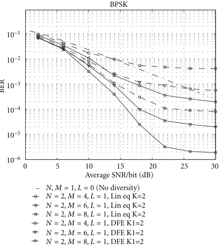
We do not provide analytical performance results for the suboptimal MIMO detectors discussed in this section. In-stead, we give results for the bit error rate (BER) obtained through computer simulations. Figure 4 shows the BER as a function of average received SNR per bit for the linear equal-izer and the DFE, respectively, in a two-path (L=1) fading channel. In both cases, the following systems were simulated: (N, M) = (2,4), (2,6), and (2,8). In the case of the linear equalizer, the filter length was 5 (K = 2). The feedforward filter lengths of the DFE were allK1=2, while the feedback
filters hadK2=L=1 coefficients.
0 5 10 15 20 25 30 Average SNR/bit (dB)
BPSK
BER
10−6 10−5 10−4 10−3 10−2 10−1
N, M=1, L=0 (No diversity) N=2, M=4, L=1, Lin eq K=2 N=2, M=6, L=1, Lin eq K=2 N=2, M=8, L=1, Lin eq K=2 N=2, M=4, L=1, DFE K1=2 N=2, M=6, L=1, DFE K1=2 N=2, M=8, L=1, DFE K1=2
Figure4: Performance of the MIMO linear and decision feedback
equalizers in two-path fading channels.
number of receive antennas increases from 4 to 8, thus increasing the order of diversity in the systems, the error rates are improved. With a higher order of receiver diver-sity the error floors are lowered, and it appears that in the two-path channel, the improvements in BER are approxi-mately one order of magnitude for every two receive anten-nas added. This observation is made for both detectors. We also note that the decision feedback equalizers provide im-provements of 3–5 dB over the linear equalizers at a BER of 10−3.
Figure 5 shows the BER performance achieved with the simplified detectors designed specifically for the case of flat fading (L = 0). The simulation results were obtained by simulating a (2,2) system. In particular, we observe that the performance of the MMSE detector is within 0.5 dB of the “no diversity” curve, while the performance of the zero-forcing detector is about 2 dB worse, mainly due to noise en-hancement caused by the matrix inversion. The performance curves for the DD-MRC detector were obtained with both correct (known) preliminary bit decisions and actual pre-liminary decisions provided by a zero-forcing detector. With correct decisions, the performance attains the lower bound on the performance of the optimal maximum likelihood de-tector, which we expect since interchannel interference is completely eliminated without compromising the order of diversity. In the other case, the DD-MRC’s performance is limited by the zero-forcing detector’s inability to make reli-able decisions. We conclude that the linear detectors lose one order of diversity compared to the optimal detector on the flat fading channel.
0 5 10 15 20 25 30
Average SNR/bit (dB) BPSK
BER
10−7 10−6 10−5 10−4 10−3 10−2 10−1
N, M=1 (No diversity) N, M=2 lower bound N, M=2 zero-forcing N, M=2 MMSE
N, M=2 DD-MRC actual dec N, M=2 DD-MRC correct dec
Figure 5: Performance of the simplified MIMO detectors in flat
fading.
5. ANALYSIS OF CODED MIMO SYSTEMS
In this section, we turn our attention to coded MIMO tems. Error correcting codes may be applied to MIMO sys-tems to improve the performance in fading and mitigate the degradation resulting from interchannel interference. Al-though there exist the so-called space-time codes which have been developed specifically for MIMO systems, any (n, k) convolutional code or block code may in principle be ap-plied to improve the performance. In the MIMO systems that we consider here, the data are encoded with a con-volutional code and interleaved before they are transmit-ted over spatially distributransmit-ted fading multipath channels. This scheme resembles a serially concatenated convolutional code (SCCC), where the convolutional code is the outer code and the MIMO multipath channel takes on the role of an in-ner time-varying convolutional code. In realizing this resem-blance, we may analyze the performance of MIMO systems using the same bounding techniques as developed previously for SCCCs [33, 34, 35].
5.1. The union bound for coded MIMO systems
beginning and the end of the codeword, we construct an equivalent block code. Thus, we may process the received sig-nals on a codeword-by-codeword basis. The length of the in-put sequence isKRo, while the length of the SCCC codeword isK/Ri. The optimal decoder for this code is a hypothetical maximum likelihood sequence decoder which operates on a hyper-trellis where the states are pairs of states of the outer and inner codes. Although prohibitively complex due to the interleaving, we will assume ML decoding for the purpose of calculating the union bound on the bit error probability.
In [33], Benedetto et al. demonstrated that high coding gains can be obtained at very low SNRs with serially con-catenated codes, provided that the interleaver is large and the inner code is a recursive code. The outer code can be either recursive or nonrecursive. In particular, it was shown that ev-ery term of the union bound decreases asymptotically at least as rapidly asK−(do
free+1)/2, wheredo
freeis the free distance of the
outer code and·denotes the integer value. This is referred to asinterleaving gain.
We view the MIMO system shown in Figure 6 as an SCCC. In order to benefit from interleaving gain, the inner “code,” that is, the channel must be recursive. The multi-path channel can be made to appear recursive to the outer code by performing recursive precoding prior to transmis-sion. Narayanan [36] showed that the preferred precoder is of the form 1/(1 +ZR) due to the enhanced convergence properties of iterative decoders for such codes. For this rea-son and for simplicity, we will restrict our attention to a sim-ple differential precoder with polynomial 1/(1 +Z) and rate Ri=1.
In the MIMO system of Figure 6, the output sequence of the outer code is passed through a uniform interleaver before being fed to N parallel and identical precoders and modulators, where each modulator is connected to a sep-arate antenna. The N signals are then transmitted over an (N, M) channel and received byM receive antennas which are connected to an ML receiver capable of performing joint demodulation, detection and decoding. As before, the chan-nels between each transmit and receive antenna are assumed to be independently fading multipath channels, each with L+ 1 paths. In Section 3, we saw that the uncoded perfor-mance in fading multipath channels is approximated by the performance of a (1, D) system with maximal ratio combin-ing in flat fadcombin-ing. Both implicit diversity of orderL+ 1 due to channel dispersion, and explicit spatial diversity of order M contribute to the effective diversity orderD =(L+ 1)M of the uncoded system. Analogously, the performance of a coded MIMO system is approximated by the performance of an SCCC in flat fading with diversity of orderD. We use this knowledge in developing the union bound below.
Since the SCCC is a linear code, the bit error probabil-ity can be calculated under the assumption that the all-zero codeword was transmitted. We define a pairwise error event as the event in which the likelihood of a codeword with Ham-ming weighth, generated by an information word with Ham-ming weightw, is higher than the likelihood of the all-zero codeword. Assuming ML decoding and BPSK modulation, the union bound is given by (see [33])
Pb≤ K/Ri
h=1
BhPh, (56)
wherePhis the pairwise error probability in Rayleigh fading given by D=(L+ 1)M. The bit error multiplicity is expressed as
Bh=
i, j denote the number of codewords with Hamming weight jgenerated by input sequences with Ham-ming weight i of the outer and inner codes, respectively. These input-output weight spectra may be calculated using the recursive method described in [35].
ForKmuch larger than the memory of the outer convo-lutional code, (56) can be approximated by (see [33])
Pb≤K/Ri
i, j,n denote the number of codewords of weight j generated by input sequences of weighti that are formed by the concatenation ofn adjacent error events of the outer and inner codes, respectively. The free distance of the outer code is denoted bydo
free, andn
o
MandniMrefer to the maximum number of adjacent error events of the outer and inner codes, respectively.
For largeK, the dominant coefficient ofPhis the one for which the exponent ofKis maximum. We define this maxi-mum exponent as
α(h)=max w,l
&
no+ni−l−1'. (60)
In general,α(h) cannot be evaluated without specifying the outer and inner codes, but general expressions can be found for two important cases, namely (i) the exponent corre-sponding to the minimum output weight, and (ii) the overall maximum exponent.
For large values of ¯γb, the union bound is dominated by the term corresponding to the minimum value ofh, known as the free distance of the SCCC ords
free. For smaller values
of ¯γb, the union bound is dominated by terms corresponding to other values ofh. To determine what these values are, we must first find the maximum value ofα,
Bits Convolutionalencoder (
Serial to parallel
Precoder & mod. Precoder
& mod.
Precoder & mod.
. . .
1 2
N
(N, M) fading multipath
chanel . . . 1
2
M ML
receiver Bits
Figure6: Coded MIMO system.
In the case of a nonrecursive inner code, input sequences with weight 1 exist, so that an input sequence with weight lwill generate at mostlerror events in the inner code. Thus, ni≤land
αM =noM−1≥0, (62) which effectively eliminates interleaving gain.
For a recursive inner code, the minimum weight of input sequences that can generate error events is 2. Input sequences of weightlcan therefore generate at mostl/2error events, and it is shown in [33] that
αM=−
)
do
free+ 1
2
*
≤0, (63)
whenl = do
free. In this case, the exponents ofK are always
negative integers yielding interleaving gain. We can therefore conclude that the union bound is dominated by error events for whichl=do
free, that is, error events from the inner code
which generate error events in the outer code with weight equal todo
free.
5.2. Approximation of the union bound
As we have seen, calculating the union bound involves the calculation of input-output weight spectra for the con-stituent codes. The bound is dominated by a relatively small number of low-weight error events, and based on the obser-vations made above, we can find an approximation of the probability of error by considering only these events. This approach allows us to circumvent the full calculation of the weight spectra.
Benedetto et al. [33] concluded that the union bound is dominated by the error event which is associated with the maximum exponentαM. The output weight of this event is denoted by h(αM). Furthermore, they observed that the re-cursive inner code has minimum input weight 2, and the minimum output weight of such input weight-2 codewords is denoted bydi
min,2, also known as the effective free distance.
The authors suggested that it is the concatenation of such minimum weight error events that result in the dominat-ing error event with output weighth(αM). In particular, er-ror events withl=do
freeconsist ofd
o
free/2 concatenated error
events in the inner code, each with input weight 2 and out-put weightdimin,2. For even values ofdfreeo , the SCCC output
weight is therefore given by
hαM=d o
freed
i
min,2
2 . (64)
For odd values ofdo
free, the SCCC error events are
concatena-tions of several inner code error events with input weight 2 and one event with input weight 3, that is,
hαM=
do
free−3
di
min,2
2 +d
i
min,3, (65)
wheredi
min,3is the minimum output weight of codewords of
the inner code with input weight 3. Ifdi
min,3=∞, the output
weight is given by
hαM=
do
free+ 1
di
min,2
2 . (66)
However, in [37], Gray claimed that the concatenation ofdo
free/2 error events from the inner code, each with output
weightdi
min,2, is not guaranteed to be the most likely error
event withl=do
free. There may be other and more likely
in-ner code error events which also have input weightdo
free. Our
approach here is to consider all concatenated error events of the inner code that have input weightl∗=dfreeo , regardless of the specific minimum-weight error events they consist of. If no such events exist in the inner code, we must consider error events with input weightl∗=do
free+ 1 or, if necessary, higher.
The procedure can be simplified by considering only con-catenated events composed of error events with minimum output weight di
min, j, where j = 2,3, . . .. With this simpli-fication there is a risk that certain compound events with h > dsfreeare missed, but the risk is justified by the simpli-fied calculations.
The union bound can now be approximated using only the multiplicity factorsBh that correspond to the particular values ofhassociated with the concatenated error events dis-cussed above, that is,
Bh≈ k
w=1
w KRo·
ACo w,l∗·ACl∗i,h
K l∗
. (67)
The value of ACo
w,l∗ is found from the input-output weight spectrum of the outer code, while the value ofACi
that consists ofniadjacent events in a block of sizeK, can be obtained in
K ni
= K!
ni!K−ni! < Kni
ni! (68) ways. This quantity includes overlapping events, but these can be ignored ifK is much greater thanniand the length of the events. Also utilizing the inequality
K l∗
< K l∗
l∗!, (69) we arrive at our final approximation ofBh,
Bh≈ k
w=1
w RoA
Co w,l∗
l∗! ni!K
ni−l∗−1
, (70)
whereni≤ l∗/2, as stated previously.
In order to calculate the bit error multiplicity given by (70), we must find the distancesdi
min, j for various values of j. In most cases, this can be done by inspection of the trellis of the inner code. As an example, consider the (2,2) system that uses a rate-1/2 nonrecursive terminated convolutional code with generating polynomial (5,7)8as outer code and a
rate-1 differential code as inner code. The outer code has a free distance ofdfreeo =5. Hence, the maximum exponent of K isαM =−3. For this particular system, we realize that the dominant error event hasl∗ =6, and the minimum output weight for the input weight-2 error events in the inner code isdi
min,2 =d
i
free=1. Sinced
i
min,3 =∞in this case, the
dom-inating output weight ish(αM)=3. From the input-output weight spectrum of the outer code we find that
ACo
2,6=K−7, (71)
and that only a single input weight (w=2) is associated with the output weightl∗ =6, causing the summation overwin (70) to vanish. Hence, the bit error probability is approxi-mated by just one term,
Pb≈B3P3, (72)
where
B3≈480(K−7)K−4, (73)
andP3is given by (57) withh=3.
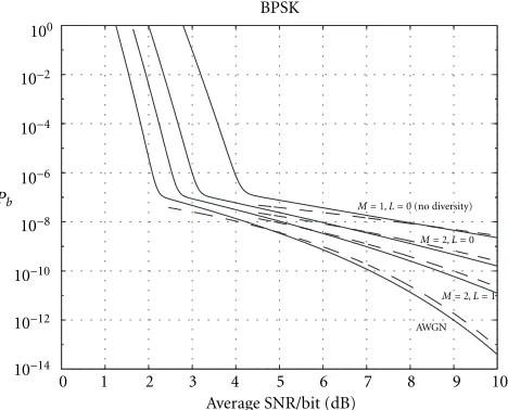
Figure 7 shows the bit error probability versus the aver-age SNR per bit, ¯γb, for a (2,2) system with an interleaver of lengthK = 512, calculated using the union bound in (56) as well as the approximate result in (72). The figure shows the error probability in a flat fading channel (L = 0, i.e., D = 2) and in a dispersive fading channel with two equal-strength paths (L = 1, i.e.,D = 4). Also shown is the per-formance of a (1,1) system in AWGN and in flat fading. As expected, the performance improves as the order of diver-sity increases. It is interesting to note that the performance
0 1 2 3 4 5 6 7 8 9 10
Average SNR/bit (dB) BPSK
Pb
10−14 10−12 10−10 10−8 10−6 10−4 10−2 100
AWGN M=2, L=1 M=2, L=0
M=1, L=0 (no diversity)
Figure7: Union bounds for coded (2,2) systems in fading.Rs =
1/2,do
free = 5,K = 512. Approximate bounds shown as dashed
curves.
of the MIMO system with diversity of orderD=4 is only 1– 2 dB worse than the performance in AWGN for SNRs lower than 10 dB. Note that the union bound diverges for values of
¯
γbless than 2.46 dB in AWGN and 4.52 dB in Rayleigh fad-ing. These values correspond to the cutoffrate for a rate-1/2 code in AWGN and fading, respectively. The rather curious shape of the bound deserves some explanation. At medium to high SNR, the performance is dominated by only a few er-ror events of low weight, resulting in the remarkable bit erer-ror rate displayed in this region. At low SNR, however, several er-ror events of larger weight contribute to the bound and this causes the performance curve to have a different slope in the divergence region. Other techniques than the union bound-ing technique discussed here must be used to predict the per-formance in this region. A survey of such techniques can be found in the paper by Shamai and Sason [38]. We observe that the bit error probability of (72) is a good approxima-tion of the union bound above the divergence region, even though only one value ofhis used in the calculation. We con-clude that we can obtain good approximations of the bit error probability without having to calculate the full input-output spectra of the constituent codes.
6. ITERATIVE EQUALIZATION AND DECODING
`
`
` `
v(k)
{LD e( ˆdn)}Nn=1
1 2 . . . M
MIMO MAP equalizer
· · ·
. . .
−
+
−+
{LD e( ˆdn)}Nn=1
−
+ . . . . . . ˆ
b(j)=sign[LD(ˆb(j))]
Serial to parallel
Parallel to serial
(
(−1 LD
e( ˆd)
−
+
LE e( ˆd)
MAP
decoder bˆ(j) LD( ˆd)
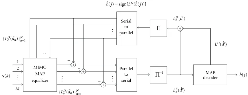
Figure8: Iterative MAP equalizer/decoder for (N, M) system.
outer convolutional code and the multipath channel, the re-ceiver performs iterative equalization and decoding. This is also known as “turbo equalization,” a technique which was first proposed by Douillard et al. in [17]. The general idea is to exploit the error correcting capabilities of the interleaved channel code to enhance the performance of the equalizer. This is accomplished by iteratively passing soft a priori in-formation between a soft-input, soft-output equalizer and a soft-input, soft-output channel decoder which are sepa-rated by an appropriate interleaver-deinterleaver pair. In this process, the reliability of the bit decisions is improved with each iteration. This is similar to the original “turbo decod-ing” principle which was first introduced by Berrou et al. in [39] for decoding of parallel concatenated codes.
As in the previous section, we consider a MIMO system which consists of an outer convolutional code followed by a pseudo-random interleaver and a differentially precoded MIMO channel. The differential precoder was chosen be-cause of its simplicity and bebe-cause it has been shown to enhance the convergence properties, and, hence, the per-formance, of the iterative equalizer/decoder [36]. The com-bination of differential precoding, modulation and multi-path channel is modeled equivalently as a MIMO recursive transversal filter. We note that the number of memory ele-ments in the precoded channel remains the same as in the nonprecoded channel. Hence, the number of states in the fi-nite state machine that characterizes the channel remains the same, while the branch transitions are altered. Since the pre-coder is a rate-1 recursive convolutional code, the data rate is not decreased. The number of states in the channel state trel-lis is 2NL, assuming binary signaling. Codewords of length NW are formed from a rate-1/ pconvolutional code which terminates in the all-zero state. These codewords are trans-mitted, received and processed as separate frames.
When employing iterative equalization and decoding in our MIMO system, the receiver structure must accommodate the passing of soft information between the equalizer and the decoder, and vice versa. We assume that the channel coeffi -cients are known or can be perfectly estimated at all times, and use a symbol-by-symbol maximum a posteriori
proba-bility (MAP) algorithm for both equalization and decoding, as shown in Figure 8. The equalizer computes a posteriori probabilities for the coded bits, based on both the received signals and a priori probabilities derived from the outputs of the channel decoder. Since we assume binary signaling, it is convenient to compute this soft information in the form of log-likelihood ratios, orL-values, which are given by
LEdn(k)ˆ =log
P{dn(k)=+1|v} P{dn(k)=−1|v}
, n=1,2, . . . , N. (74)
Here,vis the noisy received codeword
v=[v(1)v(2)· · ·v(W)]=v1W (75)
of lengthW, where{v(k)}areM-dimensional vectors, as be-fore. TheL-values contain channel information, extrinsic in-formation and a priori inin-formation. The extrinsic informa-tion is incremental informainforma-tion about the coded bit in ques-tion that has been obtained from all the other coded bits in the equalization process. Only channel information and ex-trinsic information are passed from the equalizer to the de-coder, where, after parallel-to-serial conversion and deinter-leaving, they are used as a priori information in the decoding process. This is important since, ideally, the a priori informa-tion would be provided by an independent source. We do not have access to such a source, but we may mimic the indepen-dence by minimizing the correlation between the a priori in-formation and the previous decisions made by the equalizer. This is done by subtracting the a prioriL-valuesLD
e( ˆdn(k)) from theL-values at the output of the equalizer, as shown in Figure 8
LEe
ˆ
dn(k)=LEdn(k)ˆ −LDe
ˆ
dn(k), n=1,2, . . . , N. (76)
deinterleaved coded bits. The extrinsic information to be fed back to the equalizer is obtained by subtracting the a priori information provided by the equalizer from theL-values at the output of the decoder:
LDe
ˆ
d(k)=LDdˆ(k)−LEe
ˆ
d(k). (77) The process described above constitutes one iteration and is repeated until the bit error rate converges or reaches an ac-ceptable level. The final bit decisions{b(j)}ˆ are obtained af-ter the last iaf-teration and are given by
ˆ
b(j)=signLDb(j)ˆ . (78)
6.1. The MIMO MAP equalizer
The MAP equalizer uses the well-known BCJR algorithm [40] to compute theL-valuesLE( ˆdn(k)),n=1,2, . . . , N. This algorithm optimally computes the a posteriori probabilities p(dn(k)|v) for the coded bitsdn(k), taking into account the information gathered from all theNWbits of the codeword. TheL-value for a coded bit is given by
LEdn(k)ˆ =log
wheresandsdenote the states of the channel trellis at times k−1 andk, respectively, and (s, s) denotes a transition froms tos. The summations in the numerator and the denominator are performed over all transitions which correspond to coded bitsdn(k)=+1 anddn(k)=−1, respectively.
The BCJR algorithm specifies a method for computing the probabilityp(s, s,v): probabilitiesαk(s)=p(s,v1k) are computed recursively as
αk(s)=
since we assume that the zero state is the starting state. The probabilitiesβk(s)=p(vW
k+1|s) are computed using the
back-wards recursion
where the initial conditions are
βW(s)=1 ∀s. (84) The branch transition probabilityγk(s, s) is given by
γks, s=P&s|s'·pv(k)|s, s, (85) whereP{s|s}is the a priori probability defined by
P&s|s'=
to the transition (s, s) [41]. As for the transition probability p(v(k)|s, s), we may write
whereσ2is the variance of the additive white Gaussian noise
(AWGN) [42]. Finally, combining (79), (80), (81), (82), (83), (84), (85), (86), and (87), we obtain the L-values for the coded bits
where the a prioriL-valuesL(dn(k)) are substituted with the L-valuesLD
e( ˆdn(k)) provided by the MAP decoder. 6.2. The MAP decoder
The decoder also uses the BCJR MAP algorithm to compute the a posteriori probabilities p(b(j)|v) for the information bits in the form ofL-values
whereqandqdenote the states of the code trellis at times j−1 andj, respectively.
The only difference in the computation ofL-values be-tween the decoder and the equalizer occurs in the computa-tion of the branch transicomputa-tion probabilityγj(q, q) (see [42]):
γjq, q=exp
In this expression, p is the inverse of the code rate and [d(j; 1)d(j; 2)· · ·d(j;p)] denotes the p-bit codeword pro-duced by the convolutional encoder, associated with the jth information bit. The prime denotes deinterleaved bits. We use the equalizer outputsLE
e( ˆd(j;ν)),ν=1,2, . . . , pas esti-mates for theirL-values.L(b(j)) is the a prioriL-value for the information bit b(j). The probabilitiesαj(q) andβj(q) are computed in the same way as described for the MAP equal-izer, with the following initial conditions
α0(0)=1, α0(s)=0 ∀s =0,
βNW(0)=1, βNW(s)=0 ∀s =0. (91) From (89) and (90) we obtain theL-values for the informa-tion bits
The decoder must also computeL-values for the coded bits to be fed back to the equalizer,
LDdˆ(j;ν)=log
These are computed in a similar fashion as theL-values for the information bits, yielding as final result
LDdˆ(j;ν)=Lb(j)+Ld(j;ν)
Figure9: Performance of iterative MAP decoding for a (2,2) system in flat fading (L=0). An approximate bound is shown for interme-diate SNRs.Rs=1/2,K=512.
Again, we use the equalizer outputsLE
e( ˆd(j;ν)) as estimates forL(d(j;ν)),ν = 1,2, . . . , p, andL(b(j)) is the a priori L-value for the information bitb(j). As we assume equiproba-ble information bits in our case,L(b(j))=0 in both (92) and (95).
6.3. Performance of iterative receivers
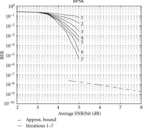
To evaluate the performance of the iterative MIMO receiver, we performed computer simulations of a (2,2) system which uses a rate-1/2, 4-state convolutional code with generator polynomial (5,7)8 anddfreeo = 5, as outer code. The coded
bits were passed through a pseudo-random interleaver of lengthK=512, serial-to-parallel converted and differentially encoded prior to transmission over a (2,2) fading channel. All simulations were carried out with BPSK modulation and with perfect knowledge of the channel coefficients. The chan-nel fading was independent from symbol interval to sym-bol interval, and the variance of the channel coefficients was σ2
f =1/D.
2 2.5 3 3.5 4 4.5 5 5.5 6 6.5 7 Average SNR/bit (dB)
BPSK
BER
10−10 10−9 10−8 10−7 10−6 10−5 10−4 10−3 10−2 10−1 100
1 1 2–4 2
3 4 5 6 7
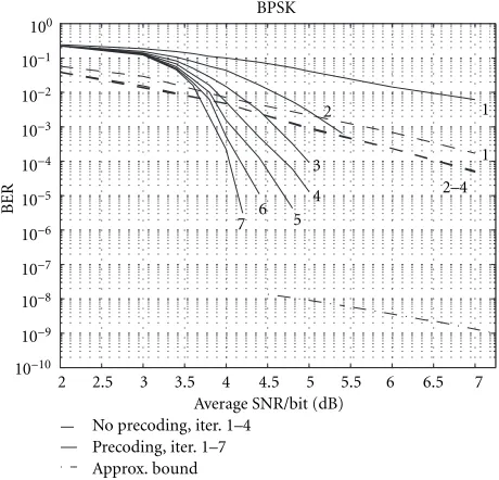
No precoding, iter. 1–4 Precoding, iter. 1–7 Approx. bound
Figure10: Performance of iterative MAP equalization and
decod-ing for a (2,2) system in a two-path fading channel with and with-out recursive precoding. An approximate bound is shown for inter-mediate SNRs.Rs=1/2,K=512.
Figure 10 contrasts the performance in a two-path (L = 1) fading channel with and without differential precoding. In particular, the dashed curves show the BER results obtained without precoding. In this case, 1– 4 iterations were per-formed. The performance improves only by approximately 1 dB after the first iteration and converges thereafter. Evi-dently, there is no interleaving gain available since the inner “code” is nonrecursive. The solid curves show the BER per-formance withdifferential precoding. In this case, the per-formance continues to show improvement, even after seven iterations. We note that the BER exhibits a dramatic drop at
¯
γb ≈4 dB, which indicates that interleaving gain due to the recursive inner “code” affects the performance. It is worth mentioning that recursive precoding results in a performance loss during the first iteration which amounts to approxi-mately 3 dB, relative to the first iteration of the nonprecoded case. This is to be expected, as differential coding is known to incur a 3 dB performance loss. Also shown is the approxi-mate analytical bound developed in Section 5.
7. CONCLUSIONS
In this paper, we have presented a general system and channel model for coded MIMO wireless systems that use multiple transmit and receive antennas. Multiple transmit anten-nas are used for the purpose of increasing the data rate, while coding and multiple receive antennas are employed to improve the performance in fading multipath channels by introducing signal diversity. For uncoded systems, we have examined the optimal MIMO MLSE detector and the suboptimal MIMO linear and decision feedback equalizers.
These detectors are fairly straightforward generalizations of their well-known single-input, single-output predecessors. We have also considered the case of flat fading and presented detectors targeted towards this special case. We have analyzed the performance of the maximum likelihood detector and found that it is capable of fully exploiting both the explicit diversity due to multiple receive antennas and implicit diver-sity due to multipath propagation. On the other hand, the suboptimal detectors are not capable of fully exploiting the diversity inherent in the channel and require many more re-ceive antennas to achieve comparable performance.
For coded MIMO systems, we have presented a theo-retical analysis of the bit error probability, assuming max-imum likelihood decoding. We have also presented a more practical iterative equalization and decoding scheme based on the BCJR MAP algorithm, and evaluated its performance through computer simulations. We have seen that by intro-ducing differential precoding, thus translating the channel into a recursive channel, significant interleaving gains can be realized compared to systems without precoding. The pro-posed receiver structure is applicable to any MIMO system which uses a convolutional code. However, as the complex-ity of trellis-based MIMO algorithms grows exponentially with the number of transmit antennas as well as the chan-nel memory, it is of interest to design receivers of lower com-plexity. Methods for complexity reduction already developed for single-input, single-output systems may be appropriately modified for this purpose.
ACKNOWLEDGMENT
This work was supported in part by the Multidisciplinary University Research Initiative (MURI) under the Office of Naval Research Contract N00014-00-1-0564.
REFERENCES
[1] G. J. Foschini and M. J. Gans, “On limits of wireless commu-nications in a fading environment when using multiple an-tennas,” Wireless Personal Communications, vol. 6, no. 3, pp. 311–335, 1998.
[2] D. Gesbert, H. B¨olcskei, D. Gore, and A. Paulraj, “MIMO wireless channels: capacity and performance prediction,” in Proc. Globecom 2000, IEEE Global Commun. Conference, pp. 1083–1088, San Francisco, Calif, USA, November 2000. [3] C. C. Martin, J. H. Winters, and N. R. Sollenberger,
“Multiple-input multiple-output (MIMO) radio channel measure-ments,” inProc. IEEE Vehicular Technology Conference (VTC-2000), Boston, Mass, USA, 2000.
[4] D. P. McNamara, M. A. Beach, P. Karlsson, and P. N. Fletcher, “Initial characterization of multiple-input multiple-output (MIMO) channels for space-time communication,” inProc. IEEE Vehicular Technology Conference (VTC-2000), Boston, Mass, USA, 2000.
[5] H. E. Nichols, A. A. Giordano, and J. G. Proakis, “MLD and MSE algorithms for adaptive detection of digital signals in the presence of interchannel interference,” IEEE Transactions on Information Theory, vol. 23, no. 5, pp. 563–575, 1977. [6] J. Salz, “Digital transmission over cross-coupled linear