The Reflected-Shifted-Truncated-Gamma Distribution for Negatively Skewed Survival Data with Application to Pediatric Nephrotic Syndrome

(1)

University of South Carolina

Scholar Commons

Theses and Dissertations

2016

Modeling of Structural Relaxation By A

Variable-Order Fractional Differential Equation

Su Yang

University of South Carolina

Follow this and additional works at:https://scholarcommons.sc.edu/etd Part of theMathematics Commons

This Open Access Thesis is brought to you by Scholar Commons. It has been accepted for inclusion in Theses and Dissertations by an authorized administrator of Scholar Commons. For more information, please [email protected].

Recommended Citation

Yang, S.(2016).Modeling of Structural Relaxation By A Variable-Order Fractional Differential Equation.(Master's thesis). Retrieved from

(2)

Modeling of structural relaxation by a variable-order fractional differential equation

by

Su Yang

Bachelor of Science

University of Science and Technology of China, 2013

Submitted in Partial Fulfillment of the Requirements

for the Degree of Master of Science in

Mathematics

College of Arts and Sciences

University of South Carolina

2016

Accepted by:

Hong Wang, Director of Thesis

Lili Ju, Reader

(3)

c

⃝ Copyright by Su Yang, 2016

(4)

Acknowledgments

Gratitude is the memory of the heart and I feel very grateful that many people

have oﬀered me valuable help for my master’s thesis, including my advisors, friends

and parents.

Firstly, I want to express my sincerest gratitude to my advisor professor Hong

Wang, who has given me much help by oﬀering me necessary materials, advice of

modifying algorithm and inspiration of new ideas with great patience and consistent

encouragement. I could not correct many mistakes and accomplish an excellent thesis

without his help. Moreover, I appreciate professor Lili Ju a lot for his advice not only

in academic but also in my life.

Then I would like to express my sincere grateful to professor Rui Xiao, my

collab-orator. I can’t finish my thesis without the experimental data he has oﬀered to me.

And he also illustrated the physical background of structural relaxation and

shape-memory behavior to me, which provided me a general idea of these two physical

processes.

Furthermore, I want to acknowledge my parents. It is really a long process from

preparing materials to finishing the thesis. I feel very happiness that my parents can

accompany with me all the time. Their help really benefited me a lot.

At last, I would like to express my gratitude to my supporter. This work was

supported in part by the National Science Foundation under Grants EAR-0934747

(5)

Abstract

In physical point of view, relaxation usually describes the return from a perturbed

system into equilibrium and each process has its own characteristic relaxation time.

In 1946, Tool first formulated the notion of fictive temperature to characterize the

structure of a glass-forming melt. Since then, people used to simulate structural

relaxation by first order model. Since fractional-based models have not widely applied

in modeling the fictive temperature, I want to explore the the possibility of modeling

structural relaxation by fractional diﬀerential equation.

In this thesis, I will first introduce the definitions of two diﬀerent kinds of fractional

derivatives: Riemann-Liouville fractional derivative and Caputo fractional derivative

briefly, and then show several existing and newly proposed models for structural

relaxation and shape-memory behavior. Finally, I will illustrate the numerical scheme

(6)

Chapter 1 background

In the field of physics, the first order evolution equation is the most widely adopted

model to describe many physical processes. It owns many advantages but at the same

time, there are many shortcomings which make the first order model not simulate

some processes well. Nowadays, as the rapidly development of fractional calculus,

more and more scholars realize that the fractional model owns advantages in

simu-lating processes with algebra decay.

In this chapter, I will instruct some general ideas of two typical processes

respec-tively, structural relaxation process and shape-memory behavior, which are usually

modeled by first order evolution equation previously.

1.1 classic model for structural relaxation

In physical point of view, relaxation is generally considered as the return of a

per-turbed system into equilibrium and each relaxation process owns characteristic with

a relaxation time t. The structural relaxation describes the relaxation in amorphous

solids.

The structural relaxation model[1] describes the transition process of glass

form-ing materials under fitted temperature. Since transition process of structure is

in-stantaneous when the temperature is higher than the softening temperature of the

glass forming material, the material always maintains in equilibrium state. When the

(9)

place quite slowly which resulting in the non-equilibrium state of glass. When the

temperature lies between the softening temperature and transition temperature, the

non-equilibrium state trends to approach to equilibrium state as the time increasing.

The time dependent transition process of structure at particular temperature can be

described as structural relaxation. In 1946, Tool introduced the fictive temperature

to describe properties of glass forming materials inside and below the glass transition

region. Tool illustrated fictive temperature of a material in a non-equilibrium state as

the real temperature of the identical material in the equilibrium state whose structure

resembles to that of the non-equilibrium material.

The first order evolution equation of fictive temperature is the most widely used

one to model structural relaxation

dTf

dt =−

Tf −T

τ (1.1)

where τ is the structural relaxation time and can be calculated as

τ(T, Tf) = τgexp

[

− C1

loge

(_C₂₍_T ₋_T_f_{) +}_T₍_T_f ₋_T_g₎

T(C2+Tf −Tg)

)]

whereτg _{is the characteristic structural relaxation time at the transition temperature}

Tg, C1, C2 are all constants.

1.2 a fractional model for structural relaxation

Since the fractional-based models have been already used in modeling

viscoelas-tic, diﬀusion problem but not throughly studied in modeling structural relaxation,

our collaborator proposed a fractional model to simulate the structural relaxation of

amorphous solids.

dαTf

dtα =−

Tf −T

τα 0< α <1 (1.2)

(10)

[

− C1

loge

(_C₂₍_T ₋_T_f_{) +}_T₍_T_f ₋_T_g₎

T(C2+Tf −Tg)

)]

whereτg is the characteristic structural relaxation time at the transition temperature

Tg, C1, C2 are all constants.

1.3 a modified fractional model for structural relaxation

In previous section, we have discussed two existing models. In this section, we are

going to present a new modified fractional model to describe the structural relaxation.

Comparing the existing fractional model in which there is only one unknown α, we

introduce a new modified model in which two parameters, α, β, are all needed to be

determined. The modified model can be expressed as

dα_T f

dtα =−

Tf −T

τβ 0< α <1,0< β <1 (1.3)

1.4 classic model for shape-memory behavior

Shape-memory polymers are particular materials which can recover to their original

state from a deformed state caused by the outer stimulation factors such as the

changing of temperature. The shape-memory behavior is introduced to describe this

kind of property.

The Zener model is widely used to describe the shape-memory property. Figure

1.1 presents a general Zener model.

(11)

Kinematics:

ϵ=ϵe+ϵv (1.4)

Constitutive relationship:

σ =Eeqϵ+Eneqϵe (1.5)

Evolution equation of internal variable:

dϵv dt =

ϵ−ϵv

τ (1.6)

Combine (1.4),(1.5),(1.6), we get a first order ODE

dϵv dt =

σ(t)−Eeqϵv

(Eneq₊_Eeq₎_τ (1.7)

where τ is a temperature-dependent relaxation time and σ is the load.

In this section, I just instruct the physical background of structural relaxation and

shape-memory behavior and their corresponding first order ODE model respectively.

However, although these first order models are widely used, the accuracy of these

models are not so satisfactory. In the following section, I will introduce some fractional

models from which we attempt to receive better numerical solutions.

1.5 a fractional model for shape-memory behavior

Since fractional diﬀerential equations simulate the heavy tail problem very well,

we try to come up with a fractional model to simulate this process.

dα_ϵv

dtα =

σ(t)−Eeq_ϵv

(Eneq₊_Eeq₎_τα (1.8)

where τ is a temperature-dependent relaxation time and σ is the load.

1.6 a modified fractional model for shape-memory behavior

In order to simulate the shape-memory behavior more accurate, we come up with

(12)

function on the entire domain. The main idea is to divide the time domain [0,T] in to

pieces and use diﬀerent fractional model to describe the property of shape-memory

behavior in each piece. In this particular problem, I just divide the entire domain

into two pieces [0,T’] and [T’,T].

The fractional model can be expressed as

dϵv dt =

σ(t)−Eeqϵv

(Eneq ₊_Eeq₎_τ 0< t < T

′ _(1.9)

dα_ϵv

dtα =

σ(t)−Eeq_ϵv

(Eneq ₊_Eeq₎_τα T

′ _{< t < T} _(1.10)

1.7 summary

In this chapter, I mainly discuss the first order ODE models and there

correspond-ing fractional models. In chapter 3, I will illustrate the inaccuracy of these first order

models and fractional models which carry out better numerical solution. Before that,

(13)

Chapter 2 numerical scheme

In this chapter, I will successively introduce the numerical scheme for first

or-der model and existing fractional model for structural relaxation and shape-memory

behavior. At the end of this chapter, I will introduce two modified fractional

mod-els which we find match the experimental data very well for structural relaxation

and shape-memory behavior respectively. Let’s begin with the first order model for

structural relaxation.

2.1 first order model for structural relaxation

Let’s first recall the first order model in chapter 1. The fictive temperature can

be expressed as

dTf

dt =−

Tf −T

τ (2.1)

where τ is the structural relaxation time and can be calculated as

[

− C1

loge

(_C₂₍_T ₋_T_f_{) +}_T₍_T_f ₋_T_g₎

T(C2+Tf −Tg)

)]

From backward diﬀerence

dTn f

dt =

Tn f −T

n−1

f

∆t ,∆t→0 (2.2)

Let’s combine (2.1) with (2.2), we can easily computeTn

f by

T_fn= ∆hT −τ T

n−1

f

(14)

2.2 first order model for shape-memory behavior

In chapter 1, we have mentioned the first order model (1.7) for shape-memory

behavior as

dϵv dt =

σ(t)−Eeqϵv

(Eneq₊_Eeq₎_τ (2.4)

By using backward diﬀerence, we can easily get the recursive formula

ϵv_n = ∆tσ(tn) + (E

eq₊_Eneq₎_{τ ϵ}v n−1

(Eeq₊_Eneq₎_τ₊_Eeq_∆_t (2.5)

2.3 a first order numerical approaches for Caputo fractional

deriva-tive

Generally speaking, we used to solve a time-fractional diﬀusion equation with

Caputo fractional derivative. In previous chapter, the two models we mentioned

are all time-fractional models. In order to achieve the numerical solution of these

equations, we are going to instruct the discrete approximation of Caputo fractional

derivative.

From formula (A.2) in appendix A, we know the definition of Caputo fractional

derivative. Then we can do the following deduction [2]:

dαT_fn dtα =

1 Γ(1−α)

∫ _t_n

0 dT_fn

dt (tn−s)

−α_ds

= 1

Γ(1−α)

n

∑

j=1

∫ jk

(j−1)k

[T_fj−T_fj−1

k +O(k)

]

(nk−s)−αds

= 1

Γ(1−α) 1 1−α

n

∑

j=1

{[T_fj −T_fj−1

k +O(k)

]

[(n−j+ 1)1−α−(n−j)1−α]}k1−α

≈ 1

Γ(1−α) 1 1−α

1 kα

n

∑

j=1

(T_fn−T_fn−1)[(n−j+ 1)1−α−(n−j)1−α]

Let’s assume

σα,k =

1 Γ(1−α)

1 1−α

1

kα and ωj =j

(15)

Then we finally have the first order approximation of Caputo fractional derivative

dα_Tn f

dtα =σα,k n

∑

j=1

ωj(T_fn−j+1−T_fn−j) +O(k) (2.6)

2.4 a fractional model for structural relaxation

In previous section, we have already deduced the numerical format for Caputo fractional

derivative. Let’s put it back to (1.2), we will get

σα,k

∑_n

j=1ωj(T_fn−j+1−T_fn−j) =− Tn

f−T

τα τασα,k

∑n

j=1ωj(Tfn−j+1−T n−j

f ) =−(Tfn−T)

Then we can get the numerical approximation forT_fn as following.

T_fn=

              

T +τασα,kω1T_f1 τα_σ

α,kω1+ 1

n= 2

T +τασα,kTfn−1−τασα,k n

∑

j=2

ωj(T_fn−j+1−T_fn−j)

τα_σ

α,kω1+ 1

n >2

(2.7)

2.5 a modified fractional order model for structural relaxation

From the numerical scheme (2.7), we can easily get the numerical scheme for the modified

model

T_fn=

              

T+τβσα,kω1Tf1

τβ_σ

α,kω1+ 1

n= 2

T+τβσα,kT_fn−1−τβσα,k n

∑

j=2

ωj(T_fn−j+1−T_fn−j)

τβ_σ

α,kω1+ 1

n >2

(2.8)

2.6 a fractional model for shape-memory behavior

(16)

ϵv_n=                       

σ(tn) +τασα,kω1ϵv1 τα_σ

α,kω1+Eeq

n= 2

σ(tn) +τασα,kϵvn−1−τασα,k n

∑

j=2

ωj(ϵvn−j+1−ϵvn−j)

τα_σ

α,kω1+Eeq

n >2

(2.9)

2.7 a modified fractional model for shape-memory behavior

As we mentioned in chapter 1, we use piecewise function to describe shape-memory

behavior. We first divide the domain of t,[0,T], into [0, tk] and [tk, T], wheretkis some grid

point. Then use first order model simulate the first piece and model with orderαto model

the second piece. The expression ofϵv_n can be written as

ϵv_n= ∆tσ(tn) + (E

eq₊_Eneq₎_{τ ϵ}v n−1

(Eeq₊_Eneq₎_τ ₊_Eeq_∆_t 0< n≤k

ϵv_n=

                      

σ(tn) +τασα,kω1ϵv1 τα_σ

α,kω1+Eeq

n=k+ 1

σ(tn) +τασα,kϵvn−1−τασα,k n

∑

j=2

ωj(ϵvn−j+1−ϵvn−j)

τα_σ

α,kω1+Eeq

n > k+ 1

(2.10)

2.8 summary

In this chapter, we expound how to deduce the numerical scheme of Caputo fractional

derivative. And in the following chapter, I am going to give some numerical experiments

to explain how to use the the numerical scheme to solve fractional models and how to

(17)

Chapter 3 numerical experiments

In this chapter, I will give some numerical examples to illustrate why the first order

model does not match the experimental data very well and then check whether existing

fractional models have better results in modeling structural relaxation and shape-memory

behavior. After that, I will present numerical investigation of modified fractional models

which may be more accurate than current fractional models.

3.1 structural relaxation

Let’s first recall the first order model in chapter 1. The fictive temperature can be

expressed as

dTf

dt =−

Tf −T

τ (3.1)

whereτ is the structural relaxation time and can be calculated as

τ(T, Tf) =τgexp

[

− C1

loge

(C2(T −Tf) +T(Tf −Tg)

T(C2+Tf−Tg)

)]

The parameters are chosen as C1 = 13.76, C2 = 32.46, τ = 900, Tg = 309K. Now let’s

further define 1/N as the grid size in time, where N is an integer. Then the grid points in

the time interval [0,T] are labledtn=nk, n= 0,1,2, ..., T ×N, where k=1/N.

(18)

270 280 290 300 310 320 330 340 295

300 305 310 315 320 325 330 335

Experimental Data

ODE

figure 3.1 Simulation by first order ODE

From figure 3.1, we can clearly see that the first order ODE model does not simulate

the experimental data very well. Then let’s take a look at fractional model. In chapter

1, we have mentioned that the fractional model can be expressed as

dαTf

dtα =−

Tf−T

τα 0< α <1 (3.2)

We can also achieve the numerical solution by iteration. Without loss of generality, we

pick α = 0.2, α = 0.5, α = 0.8 respectively and observe their accuracy by compute thing

normalized error ∥T_fα−T_fe∥L2 by the following formula

∥T_fα−Tf∥L2 =

v u u t∑N

j=0

(T_fj−T_fe(j))2 N

(19)

270 280 290 300 310 320 330 340 295

300 305 310 315 320 325 330 335

Experimental Data

ODE

Alpha=0.2

figure 3.2 Simulation by fractional model withα= 0.2

270 280 290 300 310 320 330 340 295

300 305 310 315 320 325 330 335

ODE

Alpha=0.5

(20)

270 280 290 300 310 320 330 340 295

300 305 310 315 320 325 330 335

ODE

Alpha=0.8

figure 3.4 Simulation by fractional model withα= 0.8

0.1 0.2 0.3 0.4 0.5 0.6 0.7 0.8 0.9

alpha

5 5.5 6 6.5 7 7.5 8 8.5

error

figure 3.5 The relationship between error and α

From figure 3.2, 3.3, 3.4, 3.5, it seems that as α approaches to 1, the fractional model

approaches the first order model and the error also becomes smaller and smaller as well.

(21)

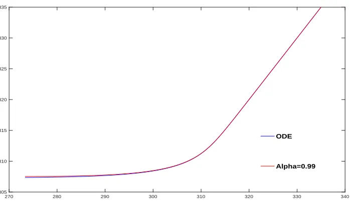
270 280 290 300 310 320 330 340 305

310 315 320 325 330 335

ODE

Alpha=0.99

figure 3.6 The comparison between ODE and α= 0.99.

Figure 3.6 shows that these two lines are almost overlapping which means the two

numerical solutions are almost equal. In another word, the fractional model does not

simulate better than the original first order model. Since these two existing models can not

accurately simulate the structural relaxation process, we come up with a modified model.

dαTf

dtα =−

Tf −T

τβ 0< α <1,0< β <1

Unlike the former fractional model, in which there is only one unknown parameter,

there exist two unknowns α and β this time. In order to determine these two unknowns

accurately, I firstly set up the region as α= [0.1,0.9] and β = [0.1,0.9]. I want to find the

minimum value of the error and its corresponding pair of α and β. Firstly, we chose

α×β = [0.1,0.9]×[0.1,0.9] and 0.1×0.1 as the grid density. Then we can obtain a 3-D

(22)

0 5 10

1 15 20 25

error

30

0.8 0.6

beta

0.4 0.3 0.2 0.1

alpha

0.4 0.2 ₀ _0.8 _0.7 0.6 0.5

0.9

figure 3.7 The relationship between α,β and error.

Figure 3.7 shows that the minimum value of error drops inα×β= [0.6,0.8]×[0.2,0.4].

Then we dense the grid in this region from 0.1×0.1 to 0.01×0.01. Then we obtain another

3-D figure as following.

0.9 0.8

alpha

0.7 0.2

0 0.5

0.22 1

1.5

0.24 2

2.5

error

0.26 3

3.5

0.28 4

0.3 4.5

beta

0.32 0.34 0.36 0.38 0.40.6

figure 3.8 The relationship between α,β and error.

We find that whenα= 0.79, β= 0.3 the outcome has the minimum error and the error

(23)

new fractional model with the experimental data and the numerical solution of ODE in a

same figure.

270 280 290 300 310 320 330 340

295 300 305 310 315 320 325 330 335

Alpha=0.79 Beta=0.3

ODE

figure 3.9 The comparison of ODE model and our model.

From figure 3.9, we can easily figure out that our new fractional model are much more

accurate in fitting the experimental data.

In previous section, we provide a general idea of structural relaxation process discuss

the accuracy of the first order ODE model. Since the ODE model does not work very well,

we then discuss the probability of a fractional model with one unknown parameterα. After

the failure of attempt to set up a fractional model with one parameter, I try to come up with

a modified fractional model with two unknownsα, β. By numerical experiments. I make

a conclusion that my new model approaches the experimental data well and I determine

the value of α, β respectively. In the coming section, I am going to introduce numerical

(24)

3.2 shape-memory behavior

Our collaborator oﬀers us the model parameters as following: C1 = 13.76, C2 =

32.46, Tg = 309, Eeq= 1.5, Eneq = 1500, A= 15000, τref = 40.

τ =

    

τref10−

C₁₍T−Tg)

C₂₊T−Tg _T _≥_T_g τref₁₀A(T1−

1

Tg) _{T < T}

g

The loading condition is chosen as:σ(t) = 0.01 ∗t, t ≤ 300;σ(t) = 0.3,300 < t ≤

980;σ(t) = 0.3−0.03(t−980),980< t≤990;σ(t) = 0, t >990.

The temperature profile is chosen as:T(t) = 333, t≤330;T(t) = 333−(t−330)/10,330<

t≤930;T(t) = 273,930< t≤1000;T(t) = 273 + (t−1000)/20, t >1000.

Applying formula (2.5) in chapter 2, we can compute the numerical solution for first

order model and fractional model and compare them with experimental data respectively.

From figure (3.10) and (3.11), we can conclude that, the first order model simulates every

well at the very beginning, but does not match the experimental data as time going on. On

contrast, the fractional model.works very well in the decay part but inaccurate in the flat

(25)

0 500 1000 1500 2000 2500 3000 -5

0 5 10 15 20 25

Experimental Data

ODE

figure 3.10 First order ODE compared with experimental data

0 500 1000 1500 2000 2500 3000

-5 0 5 10 15 20 25

Experimental Data

alpha=0.7

figure 3.11 FDE compared with experimental data

As we mentioned before, we need to divide the domain of t into two parts. For this

problem, the domain of t is [0,2630s]. After analysis the value of τ and many tries, I pick

the division point as tk = 1830s. Let’s utilize the trick mentioned in chapter 2 again to

(26)

when α = 0.5, β = 0.7). Using formula (2.10), we can compute the numerical solution in

each piece respectively.

0 500 1000 1500 2000 2500 3000

-5 0 5 10 15 20 25

Experimental Data

ODE With FDE

figure 3.12 A new method compared with experimental data

From figure 3.12, we find that our new model works more accurate than the previous

models. However, the new model still does not simulate the decaying part very well. So I

want to find some ways to improve the accuracy in this part. One way to solve this problem

is to divided the decaying part into several pieces and using diﬀerent fractional model in

each piece to simulate. Therefore, in next chapter, I am going to illustrate how to determine

(27)

Chapter 4 variable-order fractional differential

equation

In many applications, it is usually not precise to use only one fractional model with

constant order to simulate a given process. In order to improve the accuracy, we need to set

up new model with the help of variable-order fractional diﬀerential equation. In contract

to the fractional equation with constant order, the new model could change with time or

space. In this chapter, I will only discuss the model changing with time.

4.1 a variable-order fractional model

In this chapter, we always suppose to use time-fractional diﬀerential equation to simulate

a process. Let’s assume the domain of time to be [0,T] and the fractional model we use in

the following form.

dαu

dtα =a(t)u+f(t) (4.1)

The main idea in this chapter is to divide the whole domain [0,T] into pieces and use the

fractional model above to simulate the process in diﬀerent piece respectively. To simplify

the problem, we assume the order of fractional model in each piece is constant. Let N be

a positive integer, and h = 1/N be the time step. Then the grid points can be expressed

as ti = i/N, i = 0,1,2, ..., T ×N. Without loss of generality, let’s start with divide the

domain into two pieces.[0, tk] and [tk, T] and α1, α2, the orders of fractional model in each part respectively. Then the model can be described as

dα1_u

dtα1 =

σ(t)−u

(28)

dα2_u

dtα2 =

σ(t)−u

τ(t) tk≤t≤T (4.3)

In the first piece, we can just need to use (2.6) to get the approximation for Caputo

fractional derivative in this piece. The remain problem is how to get a approximation for

Caputo fractional derivative in the second piece. Since the fractional derivative is nonlocal,

we need to use the value of grid points in the first piece when computing the fractional

derivative in the second piece.

0Dαtiu= 0D

α1

tku+ tkD

α2

ti u, tk≤ti ≤T (4.4)

Let’s compute0Dtαk1uat grid point ti, i > k first.

0Dαtk1u= 1 Γ(1−α1)

∫ tk 0

du

dt(ti−s)

−α1_ds

= 1

Γ(1−α1)

k

∑

j=1

∫ jh

(j−1)h

[uj−uj−1

h +O(h)

]

(ih−s)−α1_ds

= 1

Γ(1−α1) 1 1−α1

k

∑

j=1

{[uj−uj−1

h +O(h)

]

[(i−j+ 1)1−α1 −₍_i−_j₎1−α1_]}_h1−α1

≈ 1

Γ(1−α1) 1 1−α1

1 hα1

k

∑

j=1

(uj−uj−1)[(i−j)1−α1 −(i−j−1)1−α1] Then we computetkD

α2

ti u

tkD

α2

ti u= 1 Γ(1−α2)

∫ _t_i

tk du

dt(ti−s)

−α2_ds

= 1

Γ(1−α2)

i−k

∑

j=1

∫ _jh

(j−1)h

[uk+j+1−uk+j

h +O(h)

]

(ih−s)−α2_ds

= 1

Γ(1−α2) 1 1−α2

i−_∑k−1

j=0

{[ui−j−ui−j−1

h +O(h)

]

[(j+ 1)1−α2−_j1−α2_]}_h1−α2

≈ 1

Γ(1−α2) 1 1−α2

1 hα2

i−_∑k−1

j=0

(ui−j−ui−j−1)[(j+ 1)1−α2 −j1−α2]

Combining the expression of0Dtαk1u and tkD

α2

ti u with the formula (4.4), we can get the discrete form

0Dtαiu= 1 Γ(1−α1)

1 1−α1

1 hα1

k

∑

j=1

(uj−uj−1)[(i−j)1−α1 −(i−j−1)1−α1]

+ 1

Γ(1−α2) 1 1−α2

1 hα2

i−_∑k−1

j=0

(29)

Now, Let’s put the discrete form back to (4.1)

aui+f(ti) =

1 Γ(1−α1)

1 1−α1

1 hα1

k

∑

j=1

(uj−uj−1)[(i−j)1−α1 −(i−j−1)1−α1]

+ 1

Γ(1−α2) 1 1−α2

1 hα2

i−_∑k−1

j=0

(ui−j−ui−j−1)[(j+ 1)1−α2−j1−α2]

We finally deduce the expression of ui as

ui=

[

f(ti)−σα1,h

k

∑

j=1

(uj−uj−1)[(i−j)1−α1 −(i−j−1)1−α1]

−σα2,h

i−_∑k−1

j=0

(ui−j−ui−j−1)[(j+ 1)1−α2 −j1−α2] +σα2,hui−1

]

/(σα2,h−a)

whereσαi,h = 1 Γ(2−αi)

1

hαi, i= 1,2.

We have already conclude the expression for ti, when the domain [0,T] is divided into

two pieces. To be more general, let consider the condition that [0,T] is divided into n

pieces, [t0, tk1],[tk1, tk2], ...[tkn−1, tn], wheret0 = 0, tn =T and ti drops in the m-th interval

[tkm−1, tkm], 1≤m≤n. Let’s just do some induction, we can easily find that

ui=

[

f(ti)− m_∑−1

n=1 σαn,h

kn

∑

j=kn−1

(uj−uj−1)[(i−j)1−αn−(i−j−1)1−αn]

−σα2,h

i−k∑m−1−1

j=0

(ui−j−ui−j−1)[(j+ 1)1−αm−j1−αm] +σαm,hui−1

]

(30)

Bibliography

[1] T,Nguyen, H. J.Qi, F.Castro, K.N.Long, A thermoviscoelastic model for amor-phous shape memory polymers: Incorporating structural and stress relaxation, J.Mech. Phys. Solids 56 (2008)2792-2814.

[2] D.Murio, Implicit finite diﬀerence approximation for time fractional diﬀusion equations, Computers and Mathematics with Applications 56(2008)1138-1145.

(31)

Appendix A

basic knowledge of fractional derivative

Fractional derivatives are defined via fractional integration. The fractional order

inte-gration can date back to the origin of diﬀerential calculus itself. The strict research about

fractional derivative was first worked out by Liouville in 1837.[3]

After unremitting eﬀorts in developing and modifying, various types of fractional

deriva-tives has been studied such as Rieman-Liouville, Caputo, Hadamard, Marchand, Riesz, etc.

In the following sections, I am going to pay more attentions on giving a general illustration

of Riemann-Liouville fractional derivative and Caputo fractional derivative.

A.1 Riemann-Liouville Fractional derivative

The Riemann-Liouville fractional derivative [3] is based on Riemann-Liouville fractional

integral operator which is the most widely used when computing fractional integration.

Let’s start with how to get the fractional integral operator.

Let f(x) be a function with x>0. The definite integral operator can be define as

(J f)(x) =

∫ x

0

f(t)dt

If we repeat the process, we will get

(J2f)(x) =

∫ _x

0

(J f)(t)dt=

∫ _x

0

( ∫ t

0

f(s)ds)dt

From Cauchy formula for repeated integration, we have

(Jnf)(x) = 1 (n−1)!

∫ _x

0

(x−t)n−1f(t)dt

Now, let’s replace the factorial term by Gamma function, we will get a fractional integral

(32)

(Jαf)(x) = 1 Γ(α)

∫ _x

0

(x−t)α−1f(t)dt

From the deduction above, we already have a rough frame of the Riemann-Liouville

integration operator. And the corresponding derivative is calculated as

aDtαf(t) =

dn dtn aI

n−α t f(t) =

1 Γ(α)

∫ _t

a

(t−τ)α−1f(τ)dτ, n=⌈α⌉ (A.1)

A.2 Caputo fraction derivative

Another choice for computing fractional derivative is to apply Caputo fractional

deriva-tive which was derived by M. Caputo in his paper in 1967. Diﬀerent from Riemann-Liouville

Derivative, the Caputo fractional derivative changes the order of integration operator and

derivative operator. The Caputo derivative of fractional order α of function is defined as

0Dαtf(t) =0Itn−α

dn

dtnf(t) =

1 Γ(n−α)

∫ t

0

The Reflected-Shifted-Truncated-Gamma Distribution for Negatively Skewed Survival Data with Application to Pediatric Nephrotic Syndrome

University of South Carolina

Scholar Commons

Modeling of Structural Relaxation By A

Variable-Order Fractional Differential Equation

Su Yang

Acknowledgments

Abstract

Table of Contents

Chapter 1

background

Chapter 2

numerical scheme

Chapter 3

numerical experiments

Experimental Data

ODE

Chapter 4

variable-order fractional differential

equation

Bibliography

Appendix A

basic knowledge of fractional derivative