Embedded Real-Time Architecture for
Level-Set-Based Active Contours
Eva Dejnoˇzkov ´a
Centre of Mathematical Morphology, School of Mines of Paris, 35 Rue Saint Honor´e, 77305 Fontainebleau Cedex, France Email:[email protected]
Petr Dokl ´adal
Centre of Mathematical Morphology, School of Mines of Paris, 35 Rue Saint Honor´e, 77305 Fontainebleau Cedex, France Email:[email protected]
Received 14 June 2004; Revised 5 April 2005; Recommended for Publication by Luciano da F. Costa
Methods described by partial differential equations have gained a considerable interest because of undoubtful advantages such as an easy mathematical description of the underlying physics phenomena, subpixel precision, isotropy, or direct extension to higher dimensions. Though their implementation within the level set framework offers other interesting advantages, their vast industrial deployment on embedded systems is slowed down by their considerable computational effort. This paper exploits the high parallelization potential of the operators from the level set framework and proposes a scalable, asynchronous, multiprocessor platform suitable for system-on-chip solutions. We concentrate on obtaining real-time execution capabilities. The performance is evaluated on a continuous watershed and an object-tracking application based on a simple gradient-based attraction force driving the active countour. The proposed architecture can be realized on commercially available FPGAs. It is built around general-purpose processor cores, and can run code developed with usual tools.
Keywords and phrases:level set, partial differential equations, object tracking, real-time execution, embedded platforms.
1. INTRODUCTION
The level set was proposed in 1988 in [1] as a simple method
to modelize or analyze the motion of a travelling interface.
It offers a convenient and stable framework to implement
a large variety of methods where images are seen as sets of curves. Since then, its applications have been extended to other image processing fields such as the restoration (filtering or contrast enhancement), segmentation (active contours, watershed) to the form analysis (shortest path,
shape-from-shading). See [2] or textbooks [3,4] for applications and a
general overview.
From the implementational point of view, the methods can be divided into two groups: (i) filtering-like methods op-erating on a set of constant-level curves describing the en-tire image and (ii) methods that act on a single (or several) contour(s), representing one (or several) object(s) present in the image. Below, we reference these algorithms according to
their computation scope, the filtering-like methods as
global-scope-type and the active contours methods asnarrowband type.
1.1. Scope and objectives
The objective of this paper is to open the world of hand-held, mobile devices such as PDAs, still picture or movie cameras
or mobile phones to powerful image processing methods from the level set framework. The novelty of this paper re-sides in the presentation of a reusable architecture capable to run optimally various algorithm types from the level set fam-ily. This architecture corresponds well to the system-on-chip concept, and verifies the needs of hand-held devices concern-ing their energy and implementational limitations. We par-ticularly concentrate, among other aspects, on the execution on multiprocessor, parallel, scalable architectures which is an important aspect permitting to reduce the energic consump-tion.
The rest of this paper is organized as follow. After re-viewing the state of the art of existing implementations and accelleration attempts, analyzing the family of the
level-set-based algorithms (Section 2), we present the
architec-ture (in Section 3) that best verifies the algorithmic needs
and remains efficient with respect to the HW
implementa-tion issues listed above. Its efficiency is demonstrated on a
contour-tracking algorithm proposed inSection 4.2. The text
concludes by presenting some benchmark results and general conclusions.
1.2. State of the art and technological difficulties The implicit representation of the travelling interface by
order of magnitude. A faster implementation obtained by narrowbanding the computations around the travelling
in-terface (originally called thetube method) was proposed by
Adalsteinsson et al. [5] and Malladi et al.[6]. Despite the
narrowbanding which reduces considerably the number of points to process, the level set methods remain computation-ally expensive, because of (i) using nonlinear functions, and (ii) a high number of iterations. The computational com-plexity has unpleasant consequences on both the execution time and the power consumption. If the execution time can be reduced by parallel execution (provided that the algorithm is parallelizable), the overall energy budget (following from the number of necessary operations multiplied by the energy to perform one basic operation) remains constant.
The numerous attempts to speed up the implementation of PDE-based methods made in the past were done in various axes.
(i) Algorithmic: as, for example, the implementation al-ternative to the level set, using spline-based modeling
of the contours. Precioso and Barlaud [7] have
ob-tained a fast execution on Pentium-based machines with spline-based active contours. A special care must be done to handle the topology changes. Cserey et al.
study in [8] the implementation of linear and
nonlin-ear diffusions on neural networks. In general, the
algo-rithmic modifications are often applicable to only one type of algorithms.
(ii) Mathematical: proposing a faster convergence either in another space, or using another integration scheme.
Weickert et al. propose in [9] the semi-implicit
inte-gration scheme, and the AOS scheme with arbitrarily large integration step for filters which can be written
in a specific form as in [10]. The semi-implicit scheme
increases the integration speed without affecting the
numerical stability; it deteriorates only the numerical
accuracy. Later, Goldenberg et al. [11] and Smereka
[12] use a semi-implicit scheme for the active
con-tours. However, the mathematical modifications are often applicable to only a restricted family of algo-rithms.
(iii) Hardware-based implementations are of three types. (a) Supercomputers: Holmgren and Wallin [13] use
a self-optimizing nonuniform memory access (NUMA) supercomputer implementing a high-accuracy solver for several integration kernels.
Sethian [14] has studied study flame propagation
models on a CM-2 machine with 65K processors. The author reports a true massively parallel cal-culation with one processor per grid node. (b) Graphic hardware: Rumpf and Strzodka
bene-fit from a high memory bandwidth and
imple-ment a nonlinear diffusion [15], and a level set
segmentation [16] on a graphic card. Cates et
al.[17] implement an active-contours-based
seg-mentation tool on a graphic hardware to increase the interactivity when a number of parameters must be tuned to obtain a correct segmentation
results. Sigg et al. implement a signed-distance
function transform on a graphic hardware [18].
(c) Specific HW accelerators: Hwanget al.[19] pro-pose an orthogonal architecture designed for nu-merical solution of PDEs, not inevitably related
to the image processing. It is built aroundn
pro-cessing units andn2memory blocks. Each
pro-cessor is connected to the memories by buses dedicated to only one processor, equipped with a memory access controller. The drawback of this design is that the number of interconnexions and buses increases with the square of the number of processors.
Gijbels et al. [20] propose a VLSI architecture
for nonlinear diffusion conceived for image
im-provement on image sequences. The authors use
an SIMD1architecture with distributed memory
for parallel nonlinear diffusion (i.e., the
global-scope-type) used in some vision application. The estimated performances are some 100 iterations
on a 256×256 image every 0.25 seconds, whereas
the processing units themselves are clocked at 20 MHz.
This paper focuses on the HW-based implementation
issues of the level set techniques on embedded, one-chip
devices that will be easily (i)scalable, to adapt their com-putational power to the requirements of the chosen
appli-cation, (ii) programmable with conventional programming
tools, (iii) by farless energy consuming than Pentium-based
desktop machines with comparable computational power,
and (iv) as small sized as possible. The surface occupation
is important because it has a direct impact on the price of both the chip itself and the embedding system (such as per-sonal vehicles, hand-held devices, etc.). These contraints ex-clude both the graphic hardware and supercomputer imple-mentations, since they do not match the objectives of one-chip devices, as well as the SIMD architecture, presented in
[20], which cannot be used either because of its considerable
number of used processing units (one unit per image col-umn).
Generally speaking, it is essentially due to the algorith-mic complexity that no embedded platforms have so far been proposed for the narrowband-type algorithms. The issues to handle include the following.
(i) Nonlinear computations employed in the integration
step,numerous iterationsnecessary to obtain the
con-vergence, and often required floating-point accuracy
impose using fast ALUs. Their considerable surface oc-cupation and energy consumption exclude their repli-cation in a great number on one chip.
(ii) Thedistance functioncomputation represents another
difficulty of parallelization of the narrowband
applica-tions. Dejnoˇzkov´a and Dokl´adal [21] present a detailed
analysis of existing algorithms (namely fast
Level set methods
Global-scope approach
Image morphing
•Filters:δu δt =div
g(|∇u|)∇u
•Morphological operators:δu δt = ±|∇u|
•Contour smoothing:δu δt =κ|∇u|
Narrowband approach
Image segmentaion Distance function
•Implicit contour description
|∇u| =1
•Weighted distance: continues watershed, shape-from-shading
|∇u| =Ᏺ
Deformable models
•With regularizers
•Without regularizers
•Combined (with PCA) δu
δt =Ᏺcurvature+Ᏺgradient+Ᏺregion
Figure1: PDE-based algorithms overview.
ing). It shows that they are sequential and ordered (ex-plained below). The authors propose to remove the bottleneck with the introduction of massive marching
[21]. It is a fully parallel algorithm, making use of a
nonequidistant propagation front.
Since we aim the entire algorithm family, whose common denominator is the level set implementation, the architecture has to be maximally flexible and scalable, and maximally us-ing the occupied silicon surface. The recently emergus-ing dy-namic reconfiguration represents an alternative solution to
the tradeoffbetween the functional flexibility of complex
sys-tems and the occupied surface and energy consumption, see
for example [22,23]. In some cases, the advantages of the
dy-namic reconfiguration may however be outmatched by the
drawbacks that constitute a lenghty and difficult design, the
need for special design tools [24], and external circuits
con-trolling the chip reconfiguration.
Our study demonstrates that for the level set domain, the
satisfying tradeoffbetween the flexibility and size can also be
obtained by the programmability, offered by on-chip
embed-ded processor cores and some DSP functions.
The following section presents the analysis of the ar-chitectural choices, including the computational resources, memory consistency model, and communication manage-ment. The resulting system has been synthesized for
com-mercially available FPGAs.2 Their performance becomes
al-most comparable to the ASICs.3Though the ASICs still
out-perform the FPGAs in the energy consumption (a key feature in mobile devices), the FPGAs remain a useful prototyping platform, and a possible intermediate development step to-wards an ASIC.
2. ALGORITHM ANALYSIS
This section discusses hardware implementation issues of several algorithm types from the level set context. All the
2Field-programmable gate array. 3Application-specific integrated circuit.
types consist of two basic steps: aninitializationstep that
dif-fers according to the method used, and the evolutionstep,
which makes the contour(s) travel in space and/or time
ac-cording to the given partial differential equation (PDE).
Usu-ally it makes use of some local integration kernel, and is re-peated until stability. In general, only the use of a local infor-mation is easily parallelizable. If the image is considered as a continuous signal, then the PDEs can be seen as an iteration
of a local filter operating on the neighborhood [4].
Typically, the evolution proceeds by deforming one or several curves (propagation front) or surface with a given PDE. The PDEs methods can be classified into the following
categories (cf.Figure 1).
(1) Surface propagation includesdiffusion filters[25], [26],
or [27] for a more comprehensive survey, geometric
smoothing [10,28,29], denoising, andmorphological operators[30], [31], [32] or [33] characterized by the
evolution equation∂u/∂t=F(u)|∇u|, whereu
repre-sents the evolving image. The input image reprerepre-sents
the initial conditionsu0. All points in the image are
processed in every iteration. The temporal evolution is based on the local neighborhood and generates the
evolution of the level sets in the space [4]. The
evolu-tion stops as soon the convergence or the given itera-tion number is reached.
(2) Wave propagation includes algorithms ofweighted
dis-tance, continuous watershed [34], Voronoi tesselations
[35], orshape-from-shading[36] that are controlled by
the Eikonal equation|∇u| =F. This steady-state
so-lution is propagated from the given sources (that may be obtained from the initial image by other means) on
the entire image according to the defined speedF. The
algorithm operates locally, only on the narrowband of the evolving front. The solution is propagated in waves equidistant to the sources by using ordered data struc-tures. This technique is being referred to as marching
methods, proposed by Sethian [37], as a special case of
the Dijkstra shortest-path algorithm.
End +
Convergence − Curve evolution
Initialization Start
(a)
End +
Convergence − Curve evolution
− Reconstruct NB?
+ Construction
of narrowband Initialization
Start
(b)
Figure 2: Different stages of the level set family algorithms. (a) Global-scope-type algorithms. (b)Narrowband-type algorithms.
active contours (or snakes) proposed by Kass et al.
[38] in 1987, and deformable surfaces by
Terzopou-loset al. [39] one year later. Another early example of deformable models represents the ballons by
Co-hen [40]. Implicit representation of the interface as a
constant level set of another function was studied si-multaneously and independently in 1993 by Caselles et al.[41] and Malladiet al.[42], and later by Malladi et al.[43,44,45]. The geodesic active contours were
proposed meanwhile in [46,47]. Another model was
proposed later in [48].
We distinguish the typeswith regularizers(controlled
by statistical information of regions),without
regular-izers [27], or combined with other techniques (e.g.,
principal component analysis [49]). The evolution
equation writes in the form∂u/∂t = Fcurvature(u) +
Fgrad(u) +Fregion(u). The algorithms proceed by
de-forming a given initial contour (given by u0 = 0).
The deformation is controlled by internal and external forces obtained at each iteration from (i) the contour itself and (ii) the geometrical (curvature, gradient) or statistical characteristics (mean value of the region
in-tensity) found in the image [4].
(4) Optical flow is controlled by the equations∂u/∂t =
f(∇u,I1) + g((∂I2/∂x),h), ∂v/∂t = f(∇v,I1) +
g((∂I2/∂y),h). The motion vector is obtained by
solv-ing some system of the above-given equations at each
point in the image (I1,I2are the successive sequence
images,his the searched motion vector field) [50].
Since the nature of the optical flow algorithms dif-fers from the temporal curve evolution principle of the three first groups, the proposed architecture does not address this type of algorithms. On the other hand, the optical flow often serves as a support for the three other types.
All the computation steps of the first three categories
can be unified in two following iteration types, seeFigure 2.
(1)Global-scope iteration typeincludes the surface evolution.
It operatessequentiallyon the entire image. (2)Narrowband
iteration typeincludes the wave propagation and deformable models (curve evolution).
Indeed, applying narrowbanding to the curve evolution algorithms changes the computational aspects. The points to recalculate in every iteration are now taken from some subset of the image. This set is commonly called narrowband, and contains points situated closely (up to some chosen distance) to the current position of the travelling interface. Two types of operations are commonly applied on the narrowband: (i) the curve motion scheme itself, and (ii) the (re-)construction
of the narrowband. The (re-)construction differs
substan-tially from the other algorithm types. Indeed, all HW
im-plementations of the active contours, cited inSection 1, use
fast marching; a progressive, equidistant construction of the
distance function. Fast marching itself belongs to the wave
propagationalgorithm group. It requires ordered data
struc-tures based on the priority of points [3]. From the
algorith-mical point of view, the ordering introduces a great data de-pendency, reducing the parallelization potential. From the HW implementation point of view, algorithmic ordering of
the points to process introduces random accessing to the
memory.
Parallelize the wave propagation is a tough issue, call-ing attention of many researches for a long time, compare
a survey by Roerdink and Meijster in [51]. The recent
intro-duction of massive marching opens the possibility to
paral-lelize also the computation of the distance function (cf. [52]
or [21]). Massive marching is similar to the fast
march-ing method (cf. [53] or [54]) and uses the same
entropy-satisfying upwind scheme. It differs from fast marching by
the fact that it eliminates its sorted propagation of the solu-tion and makes the implementasolu-tion fully parallelizable, with a small grain and low data dependency.
For completeness, we mention another parallelization
strategy, called group marching, developed by Kim in [55].
Group marching identifies on the front groups of points that are processed parallely in the same time. It requires nonethe-less to maintain a global variable making a truly parallel
im-plementation difficult.
The next section analyzes the execution of the different
algorithm steps by considering the use of massive march-ing for the narrowband construction. Note that the curve evolution (both algorithm types) as well as the narrowband construction (narrowband type) are time-critical. Many it-erations may be needed to obtain the convergence and the narrowband has to be reconstructed repetitively during the evolution to preserve the required properties of the implicit curve description.
2.1. Data-flow analysis of different algorithm steps In the following, we assume that, except the methods where
regularizers4 are used, the new values that the points
re-4Statistical information, like colour for example, represents global
Data
memory PU1 PU2 PU3 · · · PUn Active pointsmemory
(a)
Data
memor
y
READ
Data
memor
y
WRITE
A
cti
ve
points
memor
y
READ
A
cti
ve
points
memor
y
WRITE
Memory access type 0
0.5 1 1.5 2 2.5 3 3.5 4 4.5 5
N
u
mber
of
memor
y
ac
ce
sses
(b)
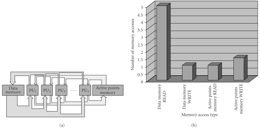
Figure3: Curve evolution implemented by using several processing units operating in parallel: (a) data-flow chart, and (b) corresponding memory accesses.
ceive are results of operations only on local neighbor-hood.
Limiting the calculations to a narrowband around the travelling contour corresponds formally to operating on sparse matrices. Practically, in order to obtain the correct evolution, all active points need to be recalculated in one iter-ation, before the next iteration starts. Therefore, unless one
uses one processing unit per point, the valuesun+1 need to
be stored separately fromun, until all the points are updated.
If this condition is verified, then the processing order is not important, and both the iteration types can be unified under
the following form. The setA, respectively, represents either
the entire image or the narrowband set:
for allpi∈Ado(in parallel)
{ Retrieve Neighborhoodun(N(pi)) andun(pi); Calculate Valueun+1(pi);
Update Valueun+1(pi);
Activate New Points(insertion inA); }
Since our constraints exclude the massive parallelism (for production cost’s reasons), we adopt a semiparallel approach instead. The data-flow chart corresponding to a semiparallel execution of this code on several processing units is given by
Figure 3a. The datauare stored in the data memory block
(two pages forunandun+1). The active points memory block
stores the setA, that is, the coordinates of the points to
pro-cess (not used for the global scope-type algorithms). The ac-tive points are read and processed by several independently operating processing units. Both the memory blocks are or-ganized in two pages, for the present one and the next itera-tion.
The width of the paths corresponds to the volumes of
transferred data. The most intensive data traffic is on the
shared blocks. The READ data memory flow is five times larger than the WRITE data memory flow because the com-plete four-neighborhood is read to update the central value (cf.Figure 3b). Similarly, since one processed point may ac-tivate several of its neighbors, the mean WRITE active points memory flow is slightly higher than READ active points memory.
The narrowbanding of active contours techniques im-pose random memory access to the data memory block.
These aspects will be taken into account inSection 3.
2.2. Timing analysis
To optimize the data flow, limit simultaneous accesses to the shared blocks, and obtain a balanced activity of all the used blocks, it is necessary to consider also the timing of the algo-rithm execution.
The global-scope type operates on the entire image, that
is, each point in the image is active and the setA=supp(I),
I = image. The narrowband type operates onA = {p |
|dist(p)| < NBwidth/2}, where NBwidth is the width of the
narrowband around the contour. For massive marching, the
definition ofAslightly differs (see [21]).
This code has two major features.
(1) The retrieval of the point’s and its neighbors’ values
un(pi) andun(N
4(pi)) requires five memory readings and is usually faster than the following calculation of
un+1(pi), which usually involves nonlinear functions.
During the calculation ofun+1(pi), the memory block
is idle.
(2) The execution of same parts of the code can have
dif-ferent length due toIF-conditions and various input
. . .
A
sync
hr
o
nous
ex
ecution
Sy
n
ch
ro
n
o
u
s
st
ar
t
PU3
PU1
PUn PU3
PU2
PU2
PUn PUn PU3
PU1
PU3
PU1
PUn PU3
PU2
PU1
PU3
PU1
PUn PU3
PU2
PU2
PUn PUn PU3
PU1
PU3
PU1
PUn PU3
PU2
PU1
Shared memory 1
Shared memory 2 PUn
· · ·
PU3
PU2
PU1 The complete processing of one point
consists of the following steps:
Retrieve pointPito process
Retrieve neighbourhoodN(Pi)
Recalculate the value ofpi (variable length) Activate other points (variable length) Update the value ofpi Wait for a shared block to become free
Figure4: Asynchronous execution of the code on four processing units (PU1to PU4) and accesses (in grey) to a shared block.
Whenever the memory is idle, it can (and should) be used to retrieve other data to process. The fact that the algorithms operate locally (using only the information from the neigh-borhood) characterizes this algorithm family by a fine granu-larity. On the other hand, the nonlinear functions categorize these algorithms rather into the medium granularity group because, in most cases, a fully functional ALU is necessary to implement the computation. These considerations impose the choice of an MIMD architecture. The processors operate
in the SPMD5mode, corresponding best to the data flow
di-agram given byFigure 3.
After a synchronous start of all the processing units, the variable length of some portions of the code gives birth to
an asynchronous execution, (cf.Figure 4). The asynchronous
execution is advantageous for parallelizable algorithms with
numerousIF-conditions, because it randomizes the access to
the shared blocks. Simultaneous accesses become rare and their HW management is easier. After the analysis of various algorithms, it becomes clear that the choice of asynchronous execution of the code on several PUs is a natural choice for the level family.
Note, that despite the asynchronous execution, the PDE-based algorithms have one or more synchronization points:
5Single program multiple data—the processors execute asynchronously
the same program.
the end of one iteration. This is indicated by either (i) empti-ness of one of the active points memory pages (narrowband-type algorithms), or (ii) end of the raster scan of the image (global scope-type algorithms). The end of the algorithm is indicated by either (i) emptiness of both active points mem-ory pages (for the narrowband-type algorithms), or (ii) the number of necessary iterations (both algorithm types), or (iii) the convergence (both algorithm types).
3. ARCHITECTURE
The image processing domain is known for various algo-rithm granularity and data dependency. Indeed, the data de-pendency and granularity are two factors that have major in-fluence on the choice of parallel implementations. Histor-ically, the fundamental model of parallel architectures has
been introduced by Flynn [56]. The further effort has been
concentrated, besides the computation resources, on the effi
-ciency of the communication configurations (see Cypher and
Sanz [57]).
The massive parallelism is efficient for regular algorithms
with fine granularity (cf. Gibbons and Rytter [58], Broggiet
al.[59] or artificial retine by Manzanera [60]). On the other
hand, if it used for random memory access implementations, the chip activity versus occupied surface will become poor. The same arguments are valid in the case of SIMD-type
CUn State vect Ctrl vect
PUn Data 32 Addr. 16 + 3 .
. . CU3 State vect
Ctrl vect
PU3 Data 32 Addr. 16 + 3 CU2 State vect
Ctrl vect
PU2 Data 32
Addr. 16 + 3 CU1 State vect
Ctrl vect
PU1 Data 32 Addr. 16 + 3
Sw
it
ch
ing
mat
rix
A
ddr
.3
Data
1
Arbitrage Semaphores
(8×1 bit)
Data 16 Data 16 Data 32 Addr. 16 Data 32 Addr. 16 Data 32 Addr. 16 Data 32 Addr. 16
LIFO (1) (32 k×16 bit)
LIFO (0) (32 k×16 bit)
A
cti
ve
points
memor
y
LABELS (65 k×16 bit)
FLAGS (65 k×1 bit)
PAGE (1) (65 k×32 bit)
PAGE (0) (65 k×32 bit)
Data
memor
y
Shared memory blocks
Figure5: Global overview of the architecture.
Hence, the image analysis community started to consider, as a possible execution platform for mean and high granular-ity algorithms, in the late 1980s, programmable,
multipro-cessor, one-chip architectures. See for example [62], [63] or
the survey of multiprocessor architectures with shared and
distributed memory [64]. For another example and
addi-tional references, see a motion estimation on a set of video
signal processors by De Greefet al.[65], or watershed
seg-mentation in Moga et al. [66], Noguet [67], or Bieniek
[68].
The data flow of the active contours, analyzed in the pre-vious section, makes them correspond better to “weaker”
parallelism models where the design effort concentrates on
the task and data dependency decomposition, task
schedul-ing, and efficient management of accessing to shared
re-sources. The architecture template, presented in this section byFigure 5, is derived from the data-flow analysis given by
Figure 3. In the following, we detail the description of the in-dividual blocks.
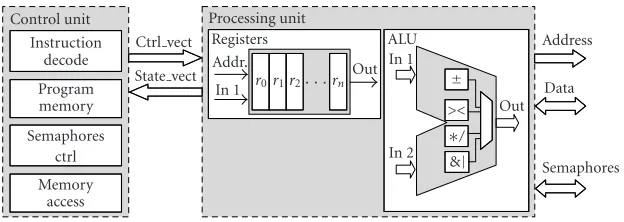
Processing and control units
The computation of the propagation speedF, which is
gen-erally a nonlinear function, is a challenge for an efficient
implementation. It seems necessary to use a fully functional arithmetic logic unit (ALU).
The processing units were realized in VHDL and Han-delC as a model of a RISC processor. They are equipped
with a set of registers. The used data word width is 32 bits to store a fixed-point data (24 + 8 the integer and fractional part).
Every processing unit is controlled by a control unit (CU). The execution of the algorithm was simulated by cod-ing the algorithm in HandelC. The advantage of this ap-proach is that the functional model can be replaced by an-other processor model or by an embedded core available on some FPGAs.
Switching matrix
The medium granularity combined with intensive random
accesses to the data memory shows that no optimum fixed
interconnection network can be found for the level set algo-rithm family. Rather than using a fixed network, one can use a switching matrix which, coupled with semaphores and ar-bitrage, permits to any processing unit access to any shared block, provided that it is not currently being used by another processing unit. Several PUs can access simultaneously to dif-ferent shared blocks.
Memory access Semaphores
ctrl Program memory Instruction
decode Control unit
Ctrl vect State vect Addr.
In 1 Registers Processing unit
r0r1r2· · ·rn
Out ALU In 1
In 2
±
><
∗/ &|
Out
Address Data
Semaphores
Figure6: Internal architecture of the processing and control units.
Figure7: The “peppers” image: (a) gradient and manually placed markers; (b) continuous watershed obtained with massive march-ing on four processmarch-ing units.
Semaphores and arbitrage
Every operation asking to access to a shared block uses the
semaphores (block semaphores ctrl at Figure 6). The code
that performs the semaphore-controlled access must respect the following:
loop :
test semaphorex // test and lock immediately if free
ifxisnot free jump loop // repeat otherwise
read/write // access to the memory
release semaphorex // release the semaphore
Whenever a semaphore is tested, it is (by the same instruc-tion) immediately locked, provided that it was free. If not, the test is repeated as long as the semaphore can be allo-cated to the asking processor. After the reading/writing, the semaphore is released. The semaphores are invisible to the user provided that the compiler generates the corresponding code.
Whenever a simultaneous access to a shared block oc-curs, an arbitrage is used to prevent conflicts. The arbi-trage is a standard block that makes part of most modern multi-processor platforms. The ideal arbitrage, usually done
on thefirst-come-first-servedbasis, and often realized as a
fi-nite state machine, is quite costly in terms of the silicium surface. We can benefit from the randomness of the asyn-chronous execution, limiting the likelihood of simultaneous accesses, and saving the space by using a simple arbitrage as-signing the processors an uneven priority. Obviously, this is only possible up to a certain number of processors however.
In this paper, we have evaluated the feasibility by measuring
the activity up to four processors (seeFigure 8showing the
activity distribution).
Data memory
A low data dependency that characterizes the level set fam-ily algorithms permits to use a simple global shared
mem-ory management, being referred to in the literature asweak
consistencymodel, introduced in [69]. The weak consistency
is characterized by three conditions (cf. [70]). (i) Before a
READ or WRITE access for any processor is allowed, all syn-chronizations must be achieved. (ii) Before a synchroniza-tion access is allowed, all previous READ or WRITE accesses must be achieved. (iii) Synchronization accesses are sequen-tially consistent with respect to each other. Note that no condition concerns the order in which the accesses are
per-formed. See [70] for details and comparison with other
con-sistency models.
The synchronization points are imposed by the iterative nature of the algorithms. All active points must be processed (in arbitrary order) in one iteration, before the following it-eration can start. This is ensured on this architecture by the fact that the data to process are read from one memory page, and the results are written to the other. As soon as all the points in one iteration are processed (all READ and WRITE
accesses are achieved), the roles of the pages PAGEs(i), i =
0,1, switch. Switching the roles of the memory pages repre-sents the synchronization.
This architecture is conceived as scalable. According to the computational power required by a given application, one can use more or fewer processing units. It follows from
Figure 3 that the highest data traffic concentrates on the shared memory blocks. Thanks to the nature of the code, the reading and writing directions on both data and active points memory blocks are separated into two one-directional
chan-nels. The results of the previous iteration (valuesun−1) are
read from one page and the new values (un) are written to
the other. This corresponds perfectly to the weak consistency model.
Active points memory
Measured Theoretical
1 2 3 4
Number of processing units used 0
5 10 15 20 25 30 35 40 45 50
M
illions
of
cl
oc
k
cy
cles
1 2
3 4
Processing unit
number
0 100 200 300 400 500 600 700
4 3
2 1
Number ofpr
ocessing units
used
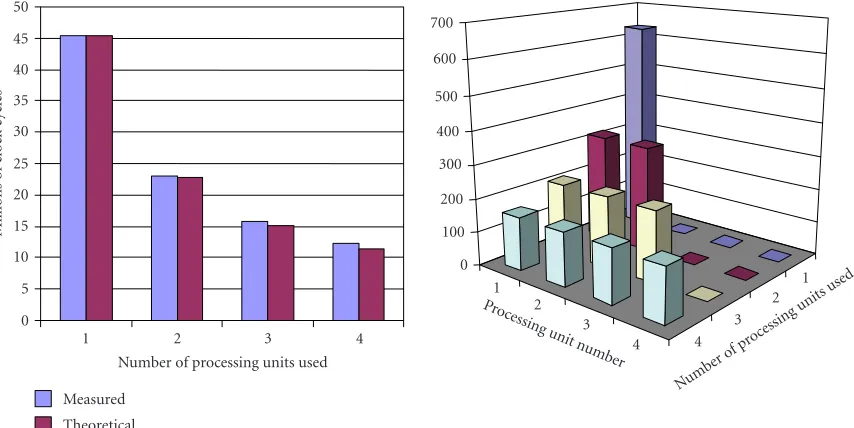
Figure8: (a) The execution time of the algorithm in function of the number of parallely working processing units. (b) The activity load distributed over several processing units, number of points processed by every processing unit (Xthousands).
to process in the current iteration. This page is progressively emptied as the data are processed. The second page contains points to process in the next iteration. It is progressively fed with data. The emptiness of one page represents the synchro-nization point. The roles of the pages (for both data and ac-tive points memory) switch. The emptiness of both acac-tive points pages represents the end of the algorithm.
The reading/writing direction to the data and active points memory blocks is controlled by using a boolean vari-ableswitchwhich commutes at the end of every iteration. For the sake of universality, it is left to the programmer’s respon-sibility to control the reading.
Thanks to the fact that the processing order is indifferent,
this memory can be implemented by using two LIFOs. Com-pared to a FIFO, using LIFO eliminates the transport delay.
For most applications, the reading should always be
done on data page(switch) and LIFO(switch) and writing on
page(switch) and LIFO(switch). The binaryswitchvalue can
be derived from the zero bit of the iteration numbern.
Flags
The labels and flags are similar to the data memory with a smaller word size. The labels and flags are available to the programmer for an additional algorithm control and region propagation.
4. PERFORMANCE EVALUATION
The performance of this architecture has been tested by
run-ning two different types of PDE-based algorithms: a
contin-uous watershed and an object-tracking application.
The objective of the watershed computation is to justify the choice to use an MIMD architecture by testing whether
the overall computational effort is uniformly distributed over
all the processors used. The objective of the tracking
applica-tion (cf.Section 4.2), is to evaluate the overall bandwidth of
the architecture, and the capability to run a computationally expensive application in real time.
4.1. Evaluation test 1: A continuous watershed implementation
Recall that, in terms of PDEs, watersheds can be obtained by calculating a weighted distance function to a given
set of sources, corresponding to the markers [34], while
propagating simultaneously the labels
∇u(x,y) = 1
∇I. (1)
Recall that the set of sources must be identical with the set
of local minima in the image, as shown in [71]. The distance
function was computed in a semiparallel way, on four paral-lely operating processing units, from a manually placed set of
markers, seeFigure 7.
Figure 8b shows the execution time (in terms of total
clock cycles against the numberNof processing units
oper-ating in parallel). The obtained number of clock cycles cor-responds to the theoretical number of clock cycles calculated
as clkN =clk1/N. The measured execution time (expressed
in terms of clock cycles) slightly exceeds the theoretical value because of the access to the shared blocks (memory, LIFO),
controlled by a semaphore.Figure??gives the computational
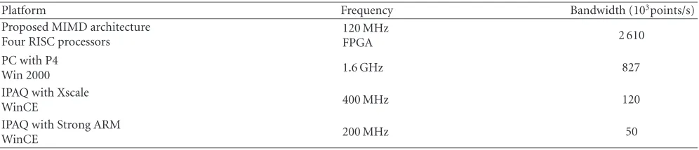
Table1: The obtained bandwidth for watershed computation versus other platforms.
Platform Frequency Bandwidth (103points/s)
Proposed MIMD architecture Four RISC processors
120 MHz
FPGA 2 610
PC with P4
Win 2000 1.6 GHz 827
IPAQ with Xscale
WinCE 400 MHz 120
IPAQ with Strong ARM
WinCE 200 MHz 50
Table 1 compares the bandwidth of weighted distance computation with simultaneous propagation of source la-bels, obtained by using massive marching implemented on various platforms. The bandwidth is computed as the num-ber of points in the image divided by the execution time. The execution time of the proposed MIMD architecture was obtained by counting the clock cycles during simulation (HandelC code). The execution time obtained on a PC/P4, IPAQ/Xscale and StrongARM corresponds to the processor time spent in the process (programmed in C).
Note that the bandwidth of every given architecture is somewhat lesser than the theoretical bandwidth because some points are activated several times. The computation
complexity of massive marching is roughlyO(N), withN
be-ing the number of points in the image. It exceedsN by the
number of reactivated points because of using a nonequidis-tant propagation front.
4.2. Evaluation test 2: Object-tracking application
To test the performance of this architecture, we use a model-free, gradient-based object-tracking algorithm
pro-posed in [72].
4.2.1. A gradient-based attraction field
Consider an imageIand some gradient ofI,g= ∇I. Let
gK=g∗K, (2)
whereKis some triangular windowZ2→R+, such that
K(x,y)=
1−αx2+y21/2 ifx2+y21/2< 1
α,
0 otherwise.
(3)
Note that in the signal processing domain, convoluting with such a window is a frequency filter. However, filtering is not the objective here.
∇gKrepresents a gradient-dependent integrator with
in-teresting properties. Generally, the evolution of a curve C
writes
∂C
∂t =Fn, (4)
wherenis the normal vector toC, andFrepresents the motion
speed. For the contour-based tracking, we propose
F = ∇gK. (5)
It can be shown (by approximatingg in (2) by a Dirac
im-pulseδ, and computingF in (5) in a discrete form) that∇gK
is a bidirectional integrator pointing towards the crest of the
gradientgfrom both sides.
The advantage of using a bidirectional integrator is twofold: (i) it allows the contour to converge towards the gra-dient maximum from both sides, and (ii) it eliminates the necessity to use a constant one-directional attraction force there, where the data is zero. This fact eliminates the problem of local breaches in the gradient, often introducing leakage in object reconstruction. Attempts to alleviate this problem
were made in [73] introducing a viscous watershed capable
to slow down the propagation in such narrow openings. Al-though the leakage could probably be alleviated by using
cur-vature, the leakage problem does not occur when using∇gK,
since on zero gradient the contour does not move.
Letφrepresent some feature of the object to track.
Sup-posing that this feature is unstable in time, or perturbed by external phenomena, one may need to employ an additional cue to enhance the stability. Natural gesture speed is one of the possible cues to track individuals. This fact is also used in defining the capture range of the contours. Suppose that the maximum interframe displacement of the object is bounded
byD. This information should be taken into account by
let-ting supp{(x,y)|K(x,y)>0}be a circle of radiusD,
gener-ating a nonzero attraction field in a narrow zone around the
contour. Hence, a convenient value ofαin (3) isa=1/D.
Indeed, as the attraction force stops on the zero cross-ing of the gradient, its principle is similar to the Haralick
[74] edge detector, which detects edges on zero crossing of
the second derivative ofIin the gradient direction. Kimmel
and Bruckstein in [75] reformulate the Haralick edge
detec-tor in terms of the level set framework and shows how it can be combined with additive constraints to segment images. As stated before, our objective is the contour-based object track-ing. Whereas various motion predictors can be used to pre-dict the displacement direction according to the past, arbi-trary deformations of the object give birth to a displacement field with locally varying direction. Any contour-based track-ing must therefore be able to handle both partially forward and backward displacements of the contour. A good overview
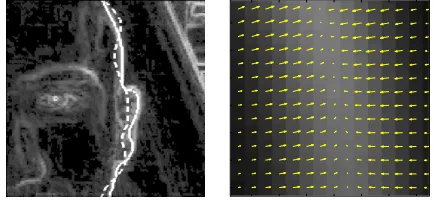
Figure9: (a) The initial (dashed) and final (solid line) position of the contour, and (b) zoom on the attraction force fieldF.
4.2.2. Application
By integrating (4), the current contourCnof the object is
ob-tained by using the attraction fieldgn
K generated by the
cur-rent frameIn, and the contourCn−1 in the previous frame
(cf.Figure 9):
Cn=lim
T→∞ T
0 ∇g n
K(C)n dt+Cn−1, (6)
withC(t=0)=Cn−1, (7)
wheregn
K=g∗K,
g(p)= ∇LabI(p)
1 +dΩ|φ(I(p)). (8)
The∇Labdenotes the gradient on the Lab colour space. The
particularity of the Lab space is that it is perceptually
uni-form, and ∇Lab is locally Euclidean. ThedΩ|φ denotes the
distance to a given feature. We use a feature based on the
skin chroma. We takeΩ ≡HLS, andφ = {x∈HLS|xH ∈
[−20o, 50o]}. This feature is only related to hue, thus the
dis-tancedHLS|φ is the angular distance dα to the skin chroma
φ. The size of the triangular windowKis ten pixels, that is,
α = 0.1, calculated from a natural gesture speed as seen by
our camera.
Initialization
The description of the initialization of the tracking is outside the scope of this paper. It can be successfully done by
com-bining several features, see for example [77], using the face
colour and shape or [78] combining the colour and motion
(in a car application, no perturbing motion is present in the background before the car runs).
4.2.3. Implementation
In the following, we outline the details concerning the im-plementation of the object tracking on the proposed archi-tecture.
This architecture has been simulated using the Han-delC programming language. The control units have been replaced by a pipelined model controlling each processing unit, equipped with a fully functional ALU realizing the ba-sic arithmetic/logic operations in fixed-point precision, and
Table2: Frame parameters.
Frame size (X×Y) 324×428
Number of points in the frame 138 672
Frames per second 15
Data flow (points per second) 2 080 080
equipped with a set of registers. The algorithms have been hardcoded in the control units in HandelC instructions. Note that every HandelC instruction is executed in one clock cycle.
Application parameters
The video stream contains 15 frames per second, each 324×
428 pixels, giving total data flow 2.08·106pixels per second
(cf.Table 2).
The narrowband width has been set to 20 points (ten to each side of the contour) and the mean length of the
con-tour of the face (cf.Figure 10) to track is approximately 600
points, giving in average 12 000 active points to update per
iteration, seeTable 3.
The above given face tracking application requires 25 it-erations in every frame for the contour to adapt itself to the new position of the face. (We consider that natural gesture speed, camera resolution, and distance to the face limit the interframe displacement of the drivers face to approximately 10 pixels.) Every five iterations, the narrowband needs to be
reinitialized (cf.Table 4).
Instruction count for various algorithm steps
The construction of the attraction force field requires one
convolution (cf. (2)). AnN×Nfast 2D convolution can be
efficiently implemented by a serie of 2N1D FFT applied to
the columns and rows,N2multiplications, and a series of 2N
1D IFFT. Efficient algorithms exist to perform FFT/IFFT in
place, see for example [79], and modern DSPs are equipped
with efficient, highly optimized blocks calculating fast the
FFT, for example [80].
We suppose that the convolution is computed on a com-panion chip. In the following, we focus on the implemen-tation of the level-set-based part of the application, that is, the (i) initialization and construction of the narrowband, (ii) contour evolution.
The gradient can be calculated with two additions and
two divisions (if central differences are used). The
attrac-tion force∇gK calculated on the entire frame requires 277,
344 additions and as many multiplications (cf.Table 5). The
construction of the narrowband, by using massive
march-ing, requires two steps: (i) the interpolationto initialize the
contour can be done with 4 additions per point and (ii) thepropagationof the distance function requires 5 additions and 6 multiplications per point. Performed twice (Jacobi and Gauss-Seidel steps) on 12 000 points (narrowband size from
Table 3) gives 216 000 additions and 144 000 multiplication required to construct the narrowband. The narrowband is reconstructed five times per frame, giving the level set
inher-ent computational effort of 1 080 000 additions and 720 000
Figure10: Contour tracking applied to driver’s face extraction, using the weighted gradient (skin chroma being the feature of interest). Randomly chosen images from a video sequence.
Table3: Narrowband parameters.
Narrow bandwidth (points) 20
Approximate mean contour length (points) 600 Number of points in the narrowband 12 000
Table4: Object-tracking application parameters.
Number of iterations before reinitialization 5
Reinitializations per frame 5
Number of iterations per frame 25
The actual curve evolution involves several steps: (i) the
evolution speedF requires 3 addition and 4 multiplications
(including the gradient of the distance function U), (ii) the integration is done in one additions and one multiplication, giving in total 4 additions and 5 multiplications per point. Multiplied by 12 000 points in the narrowband (48 000 ad-ditions and 60 000 multiplications) and by 25 iterations per
frame gives 1.2·106additions and 1.5·106multiplications
per frame. The total application effort is 2.56·106additions
and 2.50·106multiplications per frame, representing in total
75.8 MFLOPS to run in real time.
Table 6 presents the lower limits of the bandwidth
ob-tained for different steps of the object-tracking application.
The computation of the gradients∇gK and∇urequires the
same elementary operations (differences and extrema
com-putation on the neighborhood), and presents obviously the
same bandwidth 19.3·106. The limiting factor in this case
is the neighborhood extraction from the input image. We have obtained the same bandwidth estimation for the inte-gration step. The inteinte-gration does not read the neighborhood (already stored in the registers) but only writes the integra-tion result. Its performance can sometimes be limited by the bandwidth of the foregoing step.
The bandwidth 2.61·106points/s, obtained for the
nar-rowband construction, includes the detection of the initial contour position by interpolation and the propagation of the distance function.
We evaluate the performance of the architecture by com-puting the processing time of the each algorithm stage as a function of the number of processed points and these mea-sured worst-case bandwidths. The processing time of all the
steps is obtained by multiplying the worst-case bandwidth, the number of iterations, and the number of the points to process.
The sum of the processing times of individual steps gives
the frame-to-frame processing time 6.18·10−2seconds,
cor-responding to 16.3 processed frames per second.
The performance, outlined inTable 7, compares the
ex-ecution time of one iteration of the above-detailed object-tracking application on this architecture compared to simi-lar results obtained on other platforms reported in the liter-ature.
The nVIDIA GeForce2 graphic card, see [16], operates
in integer accuracy, and is therefore less useful for algorithms requiring multiple iterations. The application running on PC
P4, see [81], was implemented by using the additive operator
splitting (AOS) scheme, permitting greater integration step, and requiring thus fewer iterations.
4.3. Power assessment
As the silicium surface on FPGAs continues to grow (to be-come comparable to ASICs), the computational power is no longer a limiting factor for the design. Instead, the preoccu-pations concern more and more the energy dissipation and the system autonomy.
The energy budget of some algorithm can be character-ized by the energy necessary to execute the elementary oper-ation multiplied by the number this operoper-ation is executed. Suppose that this algorithm is to be executed in a limited time. A parallel execution (provided that the algorithm is parallelizable) will allow to reduce the clock frequency (com-pared to the clock frequency of the sequential implementa-tion) and reduce the energy budget of the elementary opera-tion.
Though it is important to take into account the energy considerations as soon as possible during the design, at this
development stage, it is still difficult to estimate precisely
the power consumption. The execution of the algorithms was simulated by using a general-purpose RISC processor model. The power consumption was then estimated by using the consumption reported by various soft-core processors
manufacturers: for Microblazer (Xilinx), see [82]; for ARM
9 family see [83]; and compared with typical-to-maximum
thermal dissipation reported for Pentium 4 at 1.6 GHz (see
Table5: Instruction count for various steps.
Instruction count for various steps Additions Multiplications
Preprocessing
∇gK(operations per point) 2 2
Total per frame (additions, multiplication) 277 344 277 344
Construction of the narrowband
Interpolation (additions, multiplications per point) 4 0
Propagation (additions, multiplications per point) 5 6
Total per initialization (additions, multiplication) 216 000 144 000
Total level-set-inherent computational effort 1 080 000 720 000
Curve evolution
Evolution speedF = ∇gK· ∇U 3 4
Integration (additions, multiplications per point)U=U−(Fdt) 1 1
Curve evolution per point (additions, multiplications) 4 5
Curve evolution per iteration (additions, multiplication) 48 000 60 000
Total curve evolution per frame 1 200 000 1 500 000
Total application per frame (curve evolution + level set inherent) 2 557 344 2 497 344
Overall real-time computational effort(FLOPS) 75.8·106
Table6: The Execution Time of the Object Tracking Application.
Algorithm step Estimated bandwidth (point/s) Number of iterations Number of points Processing time (s) Initialization
Gradient∇gK 19.3·106 1 138 672 7.19·10−3
Narrowband construction 2.61·106 5 12 000 2.30·10−2
Evolution
Gradient∇u 19.3·106 25 12 000 1.56·10−2
Integrationun+1 19.3·106 25 12 000 1.56·10−2
Total execution time (per frame) 6.13·10−2
Application frame processing rate (frame/s) 16.3
Table7: The execution time of one iteration, compared to similar algorithms on other platforms.
Platform Frequency Execution time for one iteration (ms)
Proposed MIMD architecture
Four RISC processors 120 MHz/FPGA 1.25
Graphic hardware nVIDIA GeForce2 250 MHz 4
PC with P4/Win 2000 1.6 GHz 19.1
Table8: Comparison of power consumption.
Processor Power consumption (W)
Microblazer / Xilinx 0.11
ARM9 / ARM 0.14
Pentium4 (1.6 GHz)/ Intel 60–75
5. CONCLUSIONS
In this paper, we present an embedded architecture for real-time image processing using level-set-based active contours. The contribution of this paper is twofold. In its first part, the text proposes a unifying insight into the level set framework from the system design point of view, to propose a unique
iteration type with two different types of memory access:
random memory access and sequential memory access. Then it analyzes the data flow to define, in the second part of the text, a scalable architecture fitting the real-time needs and taking into account the limited energy autonomy of em-bedded platforms and the silicium surface on commercially available FPGAs.
The performance of the proposed architecture has been studied on two benchmarks.
operating in parallel). The results show a linear increase of performance and a balanced activity at least up to four inde-pendently operating processing units.
The second benchmark implements an active-contour-based object-tracking algorithm. The purpose of this test is to evaluate the capability of this platform to run in real-time applications with intensive random memory accesses.
Section 4.2.3 lists the details concerning the computational complexity of the application in terms of number of elemen-tary operations. The simulation results show that the above-presented contour tracking application can be run on this architecture in real time, provided that the processors are clocked at 120 MHz, and one instruction executes in one clock cycle. Hence, the architecture specifications made in the first part of the text are confirmed.
The scalability of this architecture consists in replicat-ing the processreplicat-ing units. Physically, their number is lim-ited by the silicium available on the chip; and logically, by the data-flow balance on all the blocks of the archi-tecture. A time-costly computation will allow a linear in-crease of the performance up to a higher number of pro-cessing units, before the busses and the memory blocks
sat-urate. From Figure 3, it follows that the highest data flow
concentrates on the READ data memory. Although it has not been used in this paper, two possible improvements will make the data flow on the individual memory blocks more uniform: (i) the entire four-neighborhood can be re-trieved in one clock cycle by using another memory
orga-nization, as proposed by Noguet in [67], or (ii) the READ
data memory flow can be divided by two by using a dual-port memory for the data memory pages. However, both options will lead to some increase of complexity of the switch.
REFERENCES
[1] S. Osher and J. A. Sethian, “Fronts propagating with curvature-dependent speed: algorithms based on Hamilton-Jacobi formulations,” Journal of Computational Physics, vol. 79, no. 1, pp. 12–49, 1988.
[2] S. Osher and R. P. Fedkiw, “Level set methods: an overview and some recent results,”Journal of Computational Physics, vol. 169, no. 2, pp. 463–502, 2001.
[3] J. A. Sethian,Level Set Methods: Evolving Interfaces in Geom-etry, Fluid Mechanics, Computer Vision and Materials Science, Cambridge University Press, Cambridge, UK, 1996.
[4] G. Sapiro,Geometric Partial Differential Equations and Image Analysis, Cambridge University Press, New York, NY, USA, 2001.
[5] D. Adalsteinsson and J. A. Sethian, “A fast level set method for propagating interfaces,”Journal of Computational Physics, vol. 118, no. 2, pp. 269–277, 1995.
[6] R. Malladi, J. A. Sethian, and B. C. Vemuri, “A fast level set based algorithm for topology-independent shape modeling,” Journal of Mathematical Imaging and Vision, vol. 6, no. 2-3, pp. 269–289, 1996.
[7] F. Precioso and M. Barlaud, “B-spline active contour with handling of topology changes for fast video segmentation,” EURASIP Journal on Applied Signal Processing, vol. 2002, no. 6, pp. 555–560, 2002, Special Issue on Image Analysis for Multimedia Interactive.
[8] G. Cserey, C. Rekeczky, and P. F¨oldesy, “PDE-based histogram modification with embedded morphological processing of the level-sets,”Journal of Circuits, Systems and Computers, vol. 12, no. 4, pp. 519–538, 2003.
[9] J. Weickert, B. M. T. H. Romeny, and M. A. Viergever, “Effi -cient and reliable schemes for nonlinear diffusion filtering,” IEEE Trans. Image Processing, vol. 7, no. 3, pp. 398–410, 1998. [10] F. Catt´e, P.-L. Lions, J.-M. Morel, and T. Coll, “Image selec-tive smoothing and edge detection by nonlinear diffusion,” SIAM Journal on Numerical Analysis, vol. 29, no. 1, pp. 182– 193, 1992.
[11] R. Goldenberg, R. Kimmel, E. Rivlin, and M. Rudzsky, “Fast geodesic active contours,”IEEE Trans. Image Processing, vol. 10, no. 10, pp. 1467–1475, 2001.
[12] P. Smereka, “Semi-implicit level set methods for curvature and surface diffusion motion,”Journal of Scientific Comput-ing, vol. 19, no. 1-3, pp. 439–456, 2003.
[13] S. Holmgren and D. Wallin, Performance of High-Accuracy PDE Solvers on a Self-Optimizing NUMA Architecture, vol. 2150 of Lecture Notes in Computer Science, Springer, Berlin, Germany, 2001.
[14] J. A. Sethian, “Parallel level set methods for propagating inter-faces on the connection machine,” Department of Mathemat-ics, University of California at Berkeley, Berkeley, Calif, USA, 1989.
[15] M. Rumpf and R. Strzodka, “Nonlinear diffusion in graphics hardware,” inProc. EG/IEEE TCVG Symposium on Visualiza-tion (VisSym ’01 ), pp. 75–84, Ascona, Switzerland, May 2001. [16] M. Rumpf and R. Strzodka, “Level set segmentation in graph-ics hardware,” inProc. International Conference on Image Pro-cessing (ICIP ’01), vol. 3, pp. 1103–1106, Thessaloniki, Greece, October 2001.
[17] J. E. Cates, A. E. Lefohn, and R. T. Whitaker, “GIST: an inter-active, GPU-based level set segmentation tool for 3D medical images,”Medical Image Analysis, vol. 8, no. 3, pp. 217–231, 2004.
[18] C. Sigg, R. Peikert, and M. Gross, “Signed distance transform using graphics hardware,” in Proc. 14th IEEE Visualization Conference (VIS ’03), pp. 83–90, Seattle, Wash, USA, October 2003.
[19] K. Hwang, P. S. Tseng, and D. Kim, “An orthogonal multipro-cessor for parallel scientific computations,”IEEE Trans. Com-put., vol. 38, no. 1, pp. 47–61, 1989.
[20] T. Gijbels, P. Six, L. Van Gool, F. Catthoor, H. De Man, and A. Oosterlinck, “A VLSI-architecture for parallel non-linear dif-fusion with applications in vision,” inProc. IEEE Workshop on VLSI Signal Processing VII, pp. 398–407, La Jolla, Calif, USA, October 1994.
[21] E. Dejnoˇzkov´a and P. Dokl´adal, “A parallel architecture for curve-evolution PDEs,”Image Analysis and Stereology, vol. 22, pp. 121–132, 2003.
[22] R. Wittig and P. Chow, “OneChip: an FPGA processor with reconfigurable logic,” inProc. IEEE Symposium on FPGAs for Custom Computing Machines (FCCM ’96), K. L. Pocek and J. Arnold, Eds., pp. 126–135, IEEE Computer Society, Napa Val-ley, Calif, USA, April 1996.
[23] Z. A. Ye, A. Moshovos, S. Hauck, and P. Banerjee, “CHI-MAERA: a high-performance architecture with a tightly-coupled reconfigurable functional unit,” inProc. 27th Inter-national Symposium on Computer Architecture, pp. 225–235, British Columbia, Canada, 2000.