Mass imputation for two-phase sampling

4-3-2019

Mass imputation for two-phase sampling

Seho Park

Iowa State University

Jae Kwang Kim

Iowa State University

, [email protected]

Follow this and additional works at:

https://lib.dr.iastate.edu/stat_las_pubs

Part of the

Categorical Data Analysis Commons

,

Statistical Methodology Commons

, and the

Statistical Models Commons

The complete bibliographic information for this item can be found at

https://lib.dr.iastate.edu/

stat_las_pubs/256

. For information on how to cite this item, please visit

http://lib.dr.iastate.edu/

howtocite.html

.

This Article is brought to you for free and open access by the Statistics at Iowa State University Digital Repository. It has been accepted for inclusion in Statistics Publications by an authorized administrator of Iowa State University Digital Repository. For more information, please contact

Mass imputation for two-phase sampling

Abstract

Two-phase sampling is a cost-effective method of data collection using outcomedependent sampling for the

second-phase sample. In order to make efficient use of auxiliary information and to improve domain

estimation, mass imputation can be used in two-phase sampling. Rao and Sitter (1995) introduce mass

imputation for two-phase sampling and its variance estimation under simple random sampling in both phases.

In this paper, we extend the Rao–Sitter method to general sampling design. The proposed method is further

extended to mass imputation for categorical data. A limited simulation study is performed to examine the

performance of the proposed methods.

Keywords

Auxiliary information, Categorical data, Domain estimation, Outcome-dependent sampling

Disciplines

Categorical Data Analysis | Statistical Methodology | Statistical Models

Comments

This is a manuscript of an article published as S. Park and J.K. Kim (2019). "Mass imputation for two-phase

sampling",

Journal of the Korean Statistical Society. doi:

10.1016/j.jkss.2019.03.002

. Posted with permission.

Creative Commons License

This work is licensed under a

Creative Commons Attribution-Noncommercial-No Derivative Works 4.0

License

.

Contents lists available atScienceDirect

Journal of the Korean Statistical Society

journal homepage:www.elsevier.com/locate/jkss

Mass imputation for two-phase sampling

Seho Park, Jae Kwang Kim

∗

Department of Statistics, Iowa State University, Ames, IA, 50011, USA

a r t i c l e i n f o Article history: Received 6 September 2018 Accepted 13 March 2019 Available online xxxx Keywords: Auxiliary information Categorical data Domain estimation Outcome-dependent sampling

AMS 2000 subject classifications:

primary 62D05 secondary 62F40

a b s t r a c t

Two-phase sampling is a cost-effective method of data collection using outcome-dependent sampling for the second-phase sample. In order to make efficient use of auxiliary information and to improve domain estimation, mass imputation can be used in two-phase sampling. Rao and Sitter (1995) introduce mass imputation for two-phase sampling and its variance estimation under simple random sampling in both phases. In this paper, we extend the Rao–Sitter method to general sampling design. The proposed method is further extended to mass imputation for categorical data. A limited simulation study is performed to examine the performance of the proposed methods.

©2019 The Korean Statistical Society. Published by Elsevier B.V. All rights reserved.

1. Introduction

Two-phase sampling, first introduced byNeyman(1938), is a convenient and economical sampling design where the sample selection is conducted in two phases. In phase one, a large sample is collected from the target population and a relatively inexpensive auxiliary variablexis measured. In phase two, a smaller sample is drawn from the first-phase sample and the study variabley, which is expensive to measure, is collected.

Two-phase sampling or double sampling increases the precision of estimates by using auxiliary information available from the first-phase sample. Two-phase sampling is also called outcome-dependent sampling since the second-phase sampling design depends on the observations from the first-phase sampling.Hidiroglou(2001) andLegg and Fuller(2009) provided comprehensive overviews of two-phase sampling.

The structure of two-phase sampling can be seen as a missing data problem. Sincey’s are observed only in the second-phase sample and are missing in the remaining part of the first-second-phase sample, we can regard the two-second-phase sample as a planned missing data problem and apply methods for handling missing data. One popular technique is to create imputation for the missing values in the first-phase sample. It is also called as mass imputation (Kim & Rao,2012) since it requires generating a large number of imputed values.

In large-scale surveys, it is sometimes convenient or requested to produce estimates for various domains. Estimates for domains, or small area, can be computed using various techniques, including mass imputation (Moore & Robbins, 2004).Breidt, McVey, and Fuller(1996) also considered using imputation method for domain estimation under two-phase sampling and showed that the estimates obtained using mass imputation provide better estimates at finer levels of detail. Mass imputation is also applicable to survey data integration problem, in which two surveys are combined for enhanced estimation. Chipperfield, Chessman, and Lim (2012) developed mass imputation for data integration combining two independent surveys with common measurements. They considered the composite estimation after mass imputation for

∗ _{Corresponding author.}

E-mail address: [email protected](J.K. Kim).

https://doi.org/10.1016/j.jkss.2019.03.002

improved estimation.Kim and Rao(2012) also discussed mass imputation under non-nested two-phase sampling and the conditions for design consistency.

Rao and Sitter(1995) introduced a mass imputation method for two-phase sampling when both phases use the simple random sampling design. In this paper, we extend it to the complex sampling designs in each of the two phases. We propose mass imputation using a ‘‘working’’ regression model and replication variance estimation method for the mass imputation estimator. In addition, we extend the proposed method to cover categorical data mass imputation.

The rest of the paper is organized as follows. In Section 2, we introduce notation used throughout the paper and introduce two-phase regression estimator and its known properties. In Section3, we present the proposed mass imputation estimator with its asymptotic properties. In Section4, replication variance estimation for the proposed mass imputation estimator is discussed. In Section5, an extension to categorical data mass imputation is discussed and in Section6, an illustrative example is provided. Results from a simulation study is presented in Section7and concluding remarks are made in Section8.

2. Basic setup

To discuss the setup for two-phase sampling, consider a finite population, denoted byF_N

= {

(x1

,

y1)

, . . . ,

(xN

,

yN)

}

, wherexis a column vector of dimensionpandyis a scalar. LetA1denote the index set of the first-phase sample of sizen1 collected from the finite population. For the first-phase sampleA1, we assume that the first-order inclusion probability of uniti, denoted by

π

1i

=

P(i

∈

A1), is known for all elementi

∈

A1. From the first-phase sample, we select a second-phase sample by a probability sampling design with known conditional first-order inclusion probability

π

2i|1i

=

P(i

∈

A2

|

i

∈

A1). The conditional first-order inclusion probability is random in the sense that it depends on the observations from the first-phase sample. We assume that

π

2i|1iare available throughout the first-phase sample.

Let

w

1i denote the sampling weight for the first-phase sample and it is the reciprocal of the first-order inclusion probability for the first-phase sample;

w

1i

=

π

−1

1i . Also,

w

2i|1i is defined as the conditional sampling weight for the second-phase sample that is the reciprocal of the conditional inclusion probability of the second-phase sample, that is

w

2i|1i

=

π

−1 2i|1i.

We are interested in estimating the finite population total ofy, denoted byY

=

∑

N

i=1yi. When the study variableyis observed in the second-phase sample, the population totalY can be estimated using the two-phase regression estimator defined by

ˆ

Ytp,reg

= ˆ

Y2

+

(X

ˆ

1

− ˆ

X2)′

β

ˆ

, (1) whereX

ˆ

1

=

∑

i∈A1

w

1ixi, (

ˆ

X2

,

Y

ˆ

2)

=

∑

i∈A2

w

1i

w

2i|1i(xi

,

yi), and

ˆ

β

is obtained using the observations from the second-phase sample. Note that

β

is a column vector of dimensionpand notationx′

denotes the transpose ofx. To study the asymptotic properties of the two-phase regression estimator in(1), we assume a sequence of finite populations and samples defined inFuller(2009) with bounded fourth moments of (xi

,

yi). Under some regularity conditions, we can establish that

ˆ

Ytp,reg

= ˆ

Y2

+

(X

ˆ

1

− ˆ

X2) ′

β

N

+

(X

ˆ

1

− ˆ

X2) ′ (

β

ˆ

−

β

_N)

= ˆ

Y2

+

(X

ˆ

1

− ˆ

X2) ′

β

N

+

Op(n −1 2 N)

,

where

β

_Nis the probability limit of

β

ˆ

. Thus, the two-phase regression estimatorY

ˆ

tp,regis design-consistent forYregardless of the form of

β

ˆ

.

3. Proposed method

In this section, we present a new approach for mass imputation under two-phase sampling. Mass imputation estimator for the population totalY is composed of the observedyvalues of the second-phase sample and the imputed values for the rest of the first-phase sample. Thus, a mass imputation estimator for population total using a regression model is written by

ˆ

Yimp

=

∑

i∈A2

w

1iyi

+

∑

i∈ ˜A2

w

1i

ˆ

yi

,

(2) where A

˜

2

=

A1

⋂

Ac

2, y

ˆ

i

=

x′i

β

ˆ

and

β

ˆ

is to be determined later. The first component is a weighted sum of the real observations inA2and the second term is a weighted sum of imputed values inA

˜

2.

Our goal is to find a sufficient condition that makes the imputation estimator(2) algebraically equivalent to the two-phase regression estimator in(1).

Lemma 1. If

β

ˆ

satisfies

∑

i∈A2

w

1i(

w

2i|1i

−

1)(yi

−

x ′ i

β

ˆ

)

=

0

,

(3)

Proof. Condition(3)can be expressed as

∑

i∈A2

w

1i

w

i2|1(yi

− ˆ

yi)

=

∑

i∈A2

w

1i(yi

− ˆ

yi)

.

Thus,

ˆ

Yimp

=

∑

i∈A2

w

1iyi

+

∑

i∈ ˜A2

w

1iy

ˆ

i

=

∑

i∈A1

w

1iy

ˆ

i

+

∑

i∈A2

w

1i(yi

− ˆ

yi)

=

∑

i∈A1

w

1iy

ˆ

i

+

∑

i∈A2

w

1i

w

i2|1(yi

− ˆ

yi)

= ˆ

Y2

+

(X

ˆ

1

− ˆ

X2)′

β

ˆ

,

which establishes the equivalence between the mass imputation estimator and the two-phase regression estimator. ■ Note that condition(3)is satisfied if

β

ˆ

is of the form

ˆ

β

=

⎛

⎝

∑

i∈A2

w

1ixix ′ i

⎞

⎠

−1

∑

i∈A2

w

1ixiyi (4)

and

w

2i|1i

−

1 is included in the column space ofxi, which means that

w

2i|1i

−

1

=

x

′

iafor somep-dimensional vectora. Under condition(3), the mass imputation estimator(2)is also design-consistent for the population totalY. Condition(3) is similar in spirit to internal bias calibration (IBC) condition ofFirth and Bennett(1998).

The mass imputation usingy

ˆ

i as the imputed values foryican be called deterministic imputation. We can also apply the idea of fractional imputation (Fuller & Kim,2005) for mass imputation. To do this, we can write

ˆ

YFI

=

∑

i∈A2

w

1iyi

+

∑

i∈ ˜A2

w

1i(y

ˆ

i

+

∑

j∈A2

w

∗ ij

ˆ

ej)

,

(5) where

ˆ

ei

=

yi

−

x′i

β

ˆ

and

w

∗

ijis the fractional weight assigned to

ˆ

ejin uniti

∈ ˜

A2. If we choose

w

∗ ij

=

w

1j(

w

2j|1j

−

1)

/

∑

j∈A2

[

w

_1j(

w

2j|1j

−

1)

]

,

then, by(3), we have

∑

j∈A2

w

∗

ije

ˆ

j

=

0 and(5)is algebraically equivalent to the mass imputation estimator(2). By including the residual terms in the fractional imputation, we can estimate other parameters such as percentiles or distribution functions. However, it leads to have an aggregated dataset as it requires to imputen2values for one unit, so the dataset can be huge after the fractional imputation.

Note that we can express(5)as

ˆ

YFEFI

=

∑

i∈A2

w

1iyi

+

∑

i∈ ˜A2

w

1i

∑

j∈A2

w

∗ ijy ∗ ij

,

(6) wherey∗

ij

= ˆ

yi

+ ˆ

ej. Because(6)uses all possible imputed values for imputation, it can be called fully efficient fractional imputation (FEFI) estimator (Fuller & Kim,2005).

4. Replication variance estimation

In this section, we consider replication variance estimation of the mass imputation estimator in(2). Let the replicate variance estimator for the first-phase sample estimator of total be

ˆ

V1(T

ˆ

1)

=

L

∑

k=1 ck(T

ˆ

₁(k)

− ˆ

T1)2 (7) whereT

ˆ

₁(k)

=

∑

i∈A1

w

(k)

1i yi is thekth replicate of estimated totalT

ˆ

1

=

∑

i∈A1

w

1iyi,Lis the number of replications, andck

is the replication factor.

The jackknife variance estimator for the mass imputation estimator using the second-phase sample can be written as

ˆ

V(Y

ˆ

imp)

=

L

∑

k=1 ck(Y

ˆ

imp(k)

− ˆ

Yimp)2

,

(8)

where

ˆ

Y_imp(k)

=

∑

i∈A2

w

(k) 1iyi

+

∑

i∈ ˜A2

w

(k) 1ix ′ i

β

ˆ

(k) (9) and

β

ˆ

(k)

=

(

∑

i∈A2

w

(k) 1ixix′i) −1

∑

i∈A2

w

(k)

1ixiyi

.

Note thatY

ˆ

imp(k) is thekth replicate ofY

ˆ

impusing thekth replicated weight of

w

1i. We can show that the jackknife variance estimator is consistent for the variance of the mass imputation estimator. For simplicity we now assume that a Poisson sampling is used in the second-phase.Fuller(1998) argued that Poisson sampling for second-phase sample is a good approximation and has little impact on the variance estimation of the mean under two-phase sampling.

Theorem 1. Assume that a finite population of zi

=

(xi

,

yi)is a random sample from an infinite population with4

+

δ

,

δ >

0,

moments and E(

π

2i|1i)

=

κ

i. Assume that

w

2i|1i

−

1 is in the column space ofxi in computing

β

ˆ

in(4). Denote n1

= |

A1

|

,

n2

= |

A2

|

andT

ˆ

1z

=

∑

i∈A1

w

1iziis a total estimator of variable z obtained from the first-phase. Assume that

E

[| ˆ

T1z

−

T1z

|

2

|

F_N

] =

O(n−₁1N2)

,

and

V(T

ˆ

1y

|

FN)

≤

KMV(T

ˆ

y,SRS

|

FN)

,

(10)

for a fixed KM, where V(T

ˆ

y,SRS

|

FN)is the variance of the Horvitz–Thompson estimator based on a simple random sample of size

n1. Assume that the variance of a linear estimator of the total is a quadratic function of y and assume that

n1N−2V(

∑

i∈A1

w

1iyi

|

FN)

=

N

∑

i=1 N

∑

j=1 Ωijyiyj (11)

where the coefficientsΩijsatisfy N

∑

i=1

|

Ω_ij

| =

O(N−1)

.

(12)

LetV

ˆ

1(T

ˆ

1)be the first-phase sample replicate estimator of the variance ofT

ˆ

1given in(7)and satisfy

E

⎡

⎣

(

ˆ

V1(T

ˆ

1) V(_T

ˆ

₁

_|

_FN)

−

1

)

2

⏐

⏐

⏐

⏐

⏐

FN

⎤

⎦

=

o(1) (13)

for any y with bounded fourth moments. Assume that the replicates for the first-phase sample estimator of the total,T

ˆ

1, satisfy

max k E

[{

ck(T

ˆ

(k) 1

− ˆ

T1)2

}

2

|

FN

]

<

KTL −2

_[

_V(T

ˆ

1

|

FN)

]

2 (14)

for some constant KT, uniformly in N. Also, assume that max

k ck

=

O(1)

.

(15)

Then, the jackknife variance estimator of form(8)satisfies

ˆ

VJK(Y

ˆ

imp)

=

V(Y

ˆ

imp

|

FN)

−

N

∑

i=1

κ

−1 i (1

−

κ

i)e2i

+

op(n −1 2 N 2₎

_,

₍₁₆₎ where ei

=

yi

− ¯

YN

−

(xi

− ¯

XN)

β

N.

The proof ofTheorem 1is presented in the Appendix. Assumptions (10)–(12)are the regularity conditions for the variance of the Horvitz–Thompson estimator in the first-phase sample. Assumption (13)implies that the first-phase replication variance estimator is consistent and assumption(14)implies that all components of the replication variance estimator are of the same order, uniformly contribute and no component dominates the others. Assumption(15)is about the order of the replication factor and it is satisfied for the Jackknife variance estimator. These assumptions are quite standard in two-phase sampling literature and can be found inKim, Navarro, and Fuller(2006).

From (16), the bias of V

ˆ

JK(Y

ˆ

imp) is O(N) and it can be estimated unbiasedly by

∑

_i∈A2

w

1i

π

−2

2i|1i(1

−

π

2i|1i)e

ˆ

2_i

,

where

ˆ

ei

=

yi

−

x

′

i

β

ˆ

. The bias term in(16)is negligible if the first-phase sampling rate,n1

/

N, is negligible. Then, the replicate variance estimator in(8)can be used directly for the variance of mass imputation estimator under two-phase sampling.

We now consider variance estimation of the FEFI estimator in(6). Thekth replicate of the FEFI estimator is

ˆ

Y_FEFI(k)

=

∑

i∈A2

w

(k) 1iyi

+

∑

i∈ ˜A2

w

(k) 1i

∑

j∈A2

w

∗(k) ij y ∗ ij

,

(17) where

w

∗(k) ij

=

w

(k) 1j(

w

2j|1j

−

1)

/

∑

j∈A2

[

w

₁(k_j)(

w

2j|1j

−

1)

]

(18)

is the kth replicate of fractional weight. Note that the imputed values are not changed for each replication, only the fractional weights are changed. The following theorem provides the asymptotic property of the replicate variance estimator of the FEFI estimator.

Theorem 2. Assume that

ˆ

β

(k)

− ˆ

β

=

Op(n

−1

2 )

.

(19)

Then, the jackknife variance estimator of the FEFI estimator, which has a form ofV

ˆ

FEFI

=

∑

L

k=1ck(Y

ˆ

FEFI(k)

− ˆ

YFEFI)2

,

satisfies

ˆ

VFEFI

=

V(Y

ˆ

FEFI)

−

N

∑

i=1

κ

−1 i (1

−

κ

i)e2i

+

op(n −1 2 N 2₎

_,

₍₂₀₎

where

κ

i and ei are defined inTheorem1.

The proof ofTheorem 2is presented in theAppendix.

Theorem 2establishes the asymptotic equivalence of the FEFI variance estimator using(17)and the variance estimator (8) for mass imputation. By Theorem 2, the proposed FEFI variance estimator is design-consistent under two-phase sampling.

5. Categorical data mass imputation

We now extend the proposed mass imputation method to handle categorical data. Note that the regression imputation usingy

ˆ

i

=

xi

β

ˆ

does not necessarily produce imputed values belonging to the range ofyvalues and cannot be used directly to handle categoricaly-values. To discuss the problem, letytake values on

{

1

,

2

, . . . ,

K

}

. We assume a ‘‘working’’ model forP(Y

=

l

|

x):

P(Y

=

l

|

x)

=

pl(x;

β

) with

∑

K

l=1pl(x;

β

)

=

1. For example, for binaryy, we may use a logistic regression model

P(Y

=

1

|

x)

=

exp(x

′

_β

) 1

+

exp(x′

β

₎

.

Now, suppose that we are interested in estimating

θ

l

=

P(Y

=

l) from the survey data. The sampling design is the same two-phase sampling in Section2. The only difference is that the study variableyis categorical. The two-phase regression estimator of

θ

lcan be defined as

ˆ

θ

l,tp,reg

=

∑

i∈A1

w

1ipl(xi

; ˆ

β

)

+

∑

i∈A2

w

1i

π

−1 2i|1i

{

I(yi

=

l)

−

pl(xi

; ˆ

β

)

}

,

(21)

for some

β

ˆ

. Note that

θ

ˆ

l,tp,reg is design-consistent for

θ

l, regardless of whether the working model is true or not. Similarly to(2), we can construct mass imputation estimator of

θ

las follows.

ˆ

θ

l,I,reg

=

∑

i∈A2

w

1iI(yi

=

l)

+

∑

i∈ ˜A2

w

1ipl(xi

; ˆ

β

)

.

(22) Two estimators,(21)and(22), are algebraically equivalent if the following condition holds:

∑

i∈A2

w

1i

(

π

−1 2i|1i

−

1

)

{

I(yi

=

l)

−

pl(xi

; ˆ

β

)

}

=

0

.

(23)

More generally, we can use

∑

i∈A2

w

1i

(

π

−1 2i|1i

−

1

)

S(

β

ˆ

;

xi

,

yi)

=

0 (24)

as the pseudo score equation for model parameter

β

in the working modelf(y

|

x;

β

), whereS(

β

;

x

,

y)

=

∂

logf(y

|

x;

β

)

/∂

β

is the score function of

β

in the parametric working model f(y

|

x;

β

). Condition (24)is the IBC condition

Table 1

Data for the illustrative example.

Element Phase 1 Phase 1 Phase 2 Phase 2 y

ID Stratum Weight Group Weight

1 1 300 1 2 1 300 1 600 7.2 3 1 300 1 600 6.8 4 1 300 2 5 1 300 2 525 8.6 6 1 300 2 7 1 300 2 525 8.0 8 1 300 3 550 6.2 9 1 300 3 550 6.5 10 1 300 3 11 1 300 3 550 5.9 12 1 300 3 13 2 200 1 14 2 200 1 400 5.2 15 2 200 1 16 2 200 1 400 5.5 17 2 200 1 18 2 200 2 19 2 200 2 350 5.7 20 2 200 2 350 6.3 21 2 200 3 22 2 200 3 23 2 200 3 366.7 5.3 24 2 200 3 25 2 200 3 366.7 4.9 26 2 200 3 366.7 5.0

ofFirth and Bennett(1998) for the parametric model approach in two-phase sampling. It is also related to doubly robust imputation in the context of missing data imputation (Kim & Haziza,2014).

The mass imputation estimator in(22)is design-consistent under(23)but the imputed valuey

ˆ

i

=

pl(xi

; ˆ

β

) is not necessarily categorical. To create categorical imputed values and achieve design consistency, we can apply parametric fractional imputation ofKim (2011) adopted to two-phase sampling. In fractional imputation for categorical data, for each uniti

∈ ˜

A2, we createK values of (y∗ij

, w

∗

ij), forj

=

1

, . . . ,

K, wherey

∗

ij is thejth imputed value ofyi and

w

∗ij is the fractional weight assigned toy∗

ijsatisfying

∑

K j=1

w

∗

ij

=

1. In the proposed method, we usey

∗

ij

=

jand

w

∗

ij

=

pj(xi

; ˆ

β

), where

ˆ

β

satisfies(23). Using the fractionally imputed data, we can estimate

θ

lby

ˆ

θ

l,FI

=

∑

i∈A2

w

1iI(yi

=

l)

+

∑

i∈ ˜A2 K

∑

j=1

w

1i

w

∗ ijI(y ∗ ij

=

l)

.

(25)

Note that, sincey∗_ij

=

j, the fractionally imputed estimator(25)with

w

_ij∗

=

pj(xi

; ˆ

β

) is algebraically equivalent to the mass imputation estimator in(22). Because all the imputed values are categorical, the fractionally imputed dataset can be used for estimating many different parameters such as proportions.

For variance estimation, we develop replication method for fractional imputation. In fractional imputation, only the fractional weights are replicated and the imputed values are not changed for each replication. To construct thekth replicate of

w

∗

ij

=

pj(xi

; ˆ

β

), we first compute

β

ˆ

(k)

, thekth replicate of

β

ˆ

, by solving(24)with

w

1i replaced by

w

1(ki). The replication fractional weights are given by

w

_ij∗(k)

=

pj(xi

; ˆ

β

(k) ).

Using the replicated fractional weights, thekth replicate of

θ

ˆ

l,FI is obtained as

ˆ

θ

(k) l,FI

=

∑

i∈A2

w

(k) 1iI(yi

=

l)

+

∑

i∈ ˜A2 K

∑

j=1

w

(k) i1

w

∗(k) ij I(y ∗ ij

=

l) and applied to(7)to compute the variance estimator of

_θ

ˆ

_l,FI. 6. An illustrative example

In this section, we use a toy example to illustrate the mass imputation estimator and its variance estimation under two-phase sampling. The data are tabulated inTable 1, which is modified from Table 3.6 ofFuller(2009).

Suppose that the data were obtained by two-phase sampling where the first-phase sample contains 26 elements in two strata (h

=

1

,

2) and the second-phase sample contains 14 elements in three groups (g

=

1

,

2

,

3). Simple random

Table 2

Data for the illustrative example with imputed values. Element Phase 1 Phase 1 Phase 2 y∗

ID Stratum Weight Group

1 1 300 1 6.34 2 1 300 1 7.20 3 1 300 1 6.80 4 1 300 2 7.38 5 1 300 2 8.60 6 1 300 2 7.38 7 1 300 2 8.00 8 1 300 3 6.20 9 1 300 3 6.50 10 1 300 3 5.75 11 1 300 3 5.90 12 1 300 3 5.75 13 2 200 1 6.34 14 2 200 1 5.20 15 2 200 1 6.34 16 2 200 1 5.50 17 2 200 1 6.34 18 2 200 2 7.38 19 2 200 2 5.70 20 2 200 2 6.30 21 2 200 3 5.75 22 2 200 3 5.75 23 2 200 3 5.30 24 2 200 3 5.75 25 2 200 3 4.90 26 2 200 3 5.00

sampling is used in each group for selecting the second-phase sample and the second-phase sampling rate is four-in-eight, four-in-seven, and six-in-eleven, for groups 1, 2, and 3, respectively. Weights for both phases are also presented inTable 1. Letxibe the vector of covariate variable,xgi, which is an indicator variable having either 1 if elementiis in groupg, or 0 otherwise. A study variableyis continuous and observed only in the second-phase sample (A2), whereas it is missing in the remaining part of the first-phase sample (A

˜

2).

We are interested in estimating the population mean ofY,

θ

=

N−1

∑

N

i=1yi. In order to obtain the mass imputation estimator for

θ

written by

ˆ

θ

imp

=

N −1

⎛

⎝

∑

i∈A2

w

1iyi

+

∑

i∈ ˜A2

w

1iy

ˆ

i

⎞

⎠

,

(26)

the missing values ofyiinA

˜

2should be filled in by imputed values, which arey

ˆ

i

=

xi

β

ˆ

. Using Eq.(4), we can calculate

β

ˆ

from the second-phase sample given by

ˆ

β

=

⎛

⎝

∑

i∈A2

w

1ixix′i

⎞

⎠

−1

∑

i∈A2

w

1ixiyi

=

(6

.

34

,

7

.

38

,

5

.

75)

.

Then theyi’s inA

˜

2can be replaced by imputed values,y

ˆ

i

=

x

′

i

β

ˆ

, which are tabulated inTable 2. Note thaty

∗ inTable 2is defined as y∗_i

=

{

yi ifi

∈

A2

ˆ

yi ifi

∈ ˜

A2.

Then, we can obtain the mass imputation estimator by(26), which is

ˆ

θ

imp

=

N −1

⎛

⎝

∑

i∈A2

w

1iyi

+

∑

i∈ ˜A2

w

1iy

ˆ

i

⎞

⎠

=

6

.

382

.

Note that only the first-phase sample weights are used for computation of the mass imputation estimate. On the other hand, the direct expansion estimator (DEE) of

θ

is

ˆ

θ

DEE

=

⎛

⎝

∑

i∈A2

w

2i

⎞

⎠

−1

∑

i∈A2

w

2iyi

=

6

.

369

.

Variance of

θ

ˆ

impcan be estimated using Jackknife variance estimator given in(8), where thekth replicates of

θ

ˆ

impare calculated by(9). That is, leave-one-out procedure is repeated forn1

= |

A1

|

times and the

θ

ˆ

imp(k) is computed for each replicate, which is

ˆ

θ

(k) imp

=

N −1

⎛

⎝

∑

i∈A2

w

(k) 1kyi

+

∑

i∈ ˜A2

w

(k) 1iy

ˆ

(k) i

⎞

⎠

,

where

ˆ

y(_ik)

=

x′ i

β

ˆ

(k) and

β

ˆ

(k)

=

(

∑

i∈A2

w

(k) 1ixix′i

)

−1

∑

i∈A2

w

(k)

1ixiyi. Note that, for each replicate, the first-phase sample weights are changed.

Then the Jackknife variance estimate of the mass imputation estimator is obtained by

ˆ

VJK(

θ

ˆ

imp)

=

n1

∑

k=1 ck(

θ

ˆ

imp(k)

− ˆ

θ

imp)2

=

0

.

057

.

The variance estimate of the DEE estimator is 0.075.

7. Simulation study

A limited simulation study is performed to study the finite sample performance of the proposed mass imputation estimator and the replication variance estimator.

We consider two types of study variableY

=

(Y1

,

Y2), whereY1is continuous andY2is categorical.

1. Two artificial finite populations forY1 is considered: linear modely1i

=

0

.

8

+

0

.

5xi

+

zi

+

ei wherexi

∼

N(2

,

1),

ei

∼

N(0

,

1) and ratio model y1i

=

0

.

3xi

+

zi

+

ui where xi

∼

N(2

,

1) and ui

∼

N(0

,

|

xi

|

). For both models,

zi

∼

exp(1)

+

2 is used as the size measure for the unequal probability sampling in the second-phase sampling. 2 Categorical variable ofY2: we consider a binary variable ofY2

∼

Bernoulli(pi) where logit(pi)

= −

1

.

8

+

xi

+

0

.

4y1i

using they1ivalues generated from either of the artificial finite populations.

A finite population of sizeN

=

100,000 is generated from each model. From each of the finite population, first-phase samples of sizen1

=

500 are independently generated by simple random sampling. Then, second-phase samples of size

n2

=

80 are selected from the first-phase sample using the three different sampling designs as follows: (1) Simple random sampling without replacement of sizen2

=

80.

(2) Poisson sampling:

Define

δ

i for selecting unit ias

δ

i

|

Ii

=

1

∼

Bernoulli(

π

2i|1i), whereIi is an indicator variable having 1 if unit iis included in the first-phase, and having 0 otherwise. We use the conditional first-order inclusion probability of second-phase sample as

π

2i|1i

=

n2zi

/

∑

i∈A1zi, which depends on the first-phase sample, wheren2

=

80.

(3) Randomized systematic PPS sampling (RSPPS) of sizen2

=

80: We follow the procedure introduced inThompson and Wu(2008).

a. Arrange units in the first-phase sample in a random order. b. Denoteqi

=

zi

/

∑

i∈A1ziand letAj

=

∑

j

i=1n2qibe the cumulative totals ofn2qi. Note thatA0

=

0 and we have the order of 0

=

A0

<

A1

<

· · ·

<

An1

=

n2.

c. Letube a uniform random number over

[

0

,

1

]

.

d. Units with indicesjsatisfyingAj−1

≤

u

+

k

<

Ajfork

=

0

,

1

, . . . ,

n2

−

1 to be included in the second-phase sample.

Note that the first-order inclusion probability of second-phase sample

π

2i|1iobtained by the randomized systematic PPS sampling procedure satisfies

π

2i|1i

=

n2zi

/

∑

i∈A1zi, fori

∈

A1.

Once the two-phase samples are generated, we compute four estimators for the population mean

θ

=

N−1

∑

N i=1yi; (1) direct estimator, (2) classical two-phase regression estimator, (3) classical two-phase regression estimator including

π

2i|1i

−

1 as a covariate, and (4) mass imputation estimator. These estimates are defined as follows: 1. Direct estimator:

_θ

ˆ

_dir

₌

∑

i∈A2

w

1i

w

2i|1iyi

/

∑

i∈A2(

w

1i

w

2i|1i).

2. Two-phase regression estimator:

θ

ˆ

tp,reg

= ¯

y2

+

(x

¯

1

− ¯

x2)′

β

ˆ

, where

¯

x1

=

∑

i∈A1

w

1ixi

/

∑

i∈A1

w

1i

,

(x

¯

2

,

y

¯

2)

=

∑

i∈A2

w

1i

w

2i|1i(xi

,

yi)

/

∑

i∈A2 (

w

1i

w

2i|1i)

,

Table 3

Continuous case: Monte Carlo bias and Monte Carlo variance of the four estimators: Direct estimator (_θˆ_{dir); Two-phase regression estimator (θ}ˆ_{tp,reg); Two-phase regression}

estimator with extended covariates (_θˆ_{tp,reg2); Mass imputation estimator (θ}ˆ_imp).

Population Second-phase sampling Estimator Bias Variance

Linear SRS ˆ θdir 0.00 0.029 ˆ θtp,reg 0.00 0.026 ˆ θtp,reg2 0.00 0.026 ˆ θimp 0.00 0.026 Poisson ˆ θdir 0.00 0.027 ˆ θtp,reg 0.00 0.020 ˆ θtp,reg2 0.00 0.019 ˆ θimp 0.00 0.017 RSPPS ˆ θdir 0.00 0.022 ˆ θtp,reg 0.00 0.018 ˆ θtp,reg2 0.00 0.017 ˆ θimp 0.00 0.016 Ratio SRS ˆ θdir 0.00 0.040 ˆ θtp,reg 0.00 0.038 ˆ θtp,reg2 0.00 0.038 ˆ θimp 0.00 0.038 Poisson ˆ θdir 0.00 0.047 ˆ θtp,reg 0.00 0.038 ˆ θtp,reg2 0.00 0.031 ˆ θimp 0.00 0.030 RSPPS ˆ θdir 0.00 0.032 ˆ θtp,reg 0.00 0.031 ˆ θtp,reg2 0.00 0.030 ˆ θimp 0.00 0.030

ˆ

β

=

⎛

⎝

∑

i∈A2

w

1i

w

2i|1ixix ′ i

⎞

⎠

−1

∑

i∈A2

w

1i

w

2i|1ixiyi

,

andxi

=

(1

,

xi)′.

3. Two-phase regression estimator including

π

2i|1i

−

1 as a covariate:

θ

ˆ

tp,reg2

= ¯

y2

+

(x

¯

1

− ¯

x2)′

β

ˆ

, where all estimators (x

¯

1

,

x

¯

2

,

y

¯

2

,

β

ˆ

) are defined as the same with estimators in

θ

ˆ

tp,reg except forxi

=

(1

, π

2i|1i

,

xi)′.

4. Mass imputation estimator:

θ

ˆ

imp

=

N−1(

∑

i∈A2

w

1iyi

+

∑

i∈ ˜A2

w

1iy

ˆ

i), wherey

ˆ

i

=

x ′ i

β

ˆ

,

β

ˆ

=

(

∑

i∈A2

w

1ixix ′ i

)

−1

∑

i∈A2

w

1ixiyi, andxi

=

(1

, π

−1 2i|1i

,

xi)′.

Further, we compute the proposed replication variance estimator for the mass imputation estimator. The replication variance estimator of the mass imputation estimator was computed using the replication number L

=

n1. Since the first-phase sample is selected from simple random sampling of sizen1, thekth replicate weight is given by

w

(k) 1i

=

{

w

1in1

/

(n1

−

1) ifi

̸=

k

0 otherwise,

and the replication factor isck

=

(1

−

n1

/

N)(1

−

1

/

n1). This procedure was repeated 1000 times and Monte Carlo bias and variance of the four estimators, Monte Carlo coverage rate of the mass imputation estimator and Monte Carlo mean and relative bias of the replication variance estimator are computed.

Tables 3and4present the Monte Carlo bias and variance of the four estimators for continuous case (Y1) and categorical case (Y2), respectively, andTable 5presents the Monte Carlo coverage rate of the mass imputation estimator for all cases. We can check that all four point estimators are unbiased for the population mean regardless of sampling design and specified population model type. The Monte Carlo coverage rates are about 95% for all cases. Moreover, the variances of classical two-phase regression estimator, two-phase regression estimator with extended xi and mass imputation estimator for the sample selected using simple random sampling for both phases are the same, because

π

₂−_i|11iis constant under simple random sampling for the second-phase sampling. For other designs, the mass imputation estimator has smaller variance compared with the classical two-phase regression estimator as the auxiliary variable used for the mass imputation estimator contains the additional information in

π

₂−_i|11i. Because the mass imputation estimator is based on the augmented regression model, augmented by

π

₂−_i|11i, it is more efficient in the sense of reducing the variance. The mass

Table 4

Categorical case: Monte Carlo bias and Monte Carlo variance of the four estimators: Direct estimator (_θˆ_{dir); Two-phase regression estimator (θ}ˆ_{tp,reg); Two-phase regression}

estimator with extended covariates (_θˆ_{tp,reg2); Mass imputation estimator (θ}ˆ_imp).

Population Second-phase sampling Estimator Bias Variance (×105₎

Linear SRS ˆ θdir 0.00 181 ˆ θtp,reg 0.00 157 ˆ θtp,reg2 0.00 157 ˆ θimp 0.00 157 Poisson ˆ θdir 0.00 359 ˆ θtp,reg 0.00 232 ˆ θtp,reg2 0.00 206 ˆ θimp 0.00 181 RSPPS ˆ θdir 0.00 256 ˆ θtp,reg 0.00 198 ˆ θtp,reg2 0.00 197 ˆ θimp 0.00 184 Ratio SRS ˆ θdir 0.00 223 ˆ θtp,reg 0.00 189 ˆ θtp,reg2 0.00 189 ˆ θimp 0.00 189 Poisson ˆ θdir 0.00 397 ˆ θtp,reg 0.00 257 ˆ θtp,reg2 0.00 246 ˆ θimp 0.00 216 RSPPS ˆ θdir 0.00 289 ˆ θtp,reg 0.00 234 ˆ θtp,reg2 0.00 233 ˆ θimp 0.00 216 Table 5

Monte Carlo coverage rate of the mass imputation estimator.

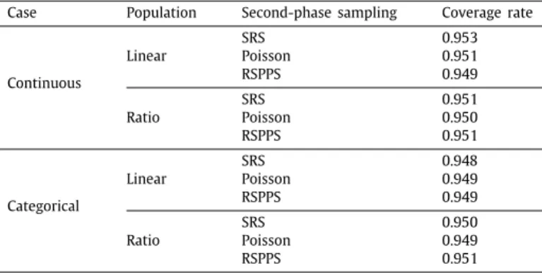
Case Population Second-phase sampling Coverage rate

Continuous Linear SRS 0.953 Poisson 0.951 RSPPS 0.949 Ratio SRS 0.951 Poisson 0.950 RSPPS 0.951 Categorical Linear SRS 0.948 Poisson 0.949 RSPPS 0.949 Ratio SRS 0.950 Poisson 0.949 RSPPS 0.951

imputation estimator is slightly more efficient than the two-phase regression estimator with extended covariates. The mass imputation estimator uses only

w

1iin computing

β

ˆ

while the two-phase regression estimator uses

w

1i

w

2i|1i, which creates extra variability in the final estimation.

Table 6presents Monte Carlo mean and relative bias of the replication variance estimator of the mass imputation estimator. The relative bias of the variance estimator is obtained by dividing Monte Carlo bias of the variance estimator by the Monte Carlo variance of the point estimator. All Monte Carlo means of the replication variance estimators are consistent for the variance of the mass imputation estimator given inTables 3and4, and it leads to small relative biases of the replication variance estimator inTable 6. This result supportsTheorem 1, as the bias term in(16)can be safely ignored since the first-phase sampling rate is 500

/

100,000

=

0

.

005, which is small enough.

8. Conclusion

We treat two-phase sampling as a missing data problem and propose a mass imputation estimator that is equivalent to the two-phase regression estimator. The proposed replication variance estimation is simple to implement since it does

Table 6

Monte Carlo mean and relative bias (R.B.) of the replication variance estimator of the mass imputation estimator.

Case Population Second-phase sampling Mean R.B.

Continuous Linear SRS 0.026 0.001 Poisson 0.017 0.003 RSPPS 0.016 0.002 Ratio SRS 0.039 0.006 Poisson 0.032 0.057 RSPPS 0.031 0.017 Categorical Linear SRS 0.0015 0.002 Poisson 0.0018 0.016 RSPPS 0.0018 −0.005 Ratio SRS 0.0019 0.028 Poisson 0.0022 0.048 RSPPS 0.0022 0.033

not require computing replicates of the conditional inclusion probability for the second-phase sample, which may be complicated or impossible to compute depending on the sampling designs. The proposed method is further extended to categorical data mass imputation.

In mass imputation, to achieve design consistency, we have used an augmented regression model for imputation by including the inverse of the conditional inclusion probability for the second-phase sample into the covariates. Thus, the proposed method is applicable only when the conditional inclusion probabilities are available throughout the first-phase sample. If all the design information for the second-first-phase sampling is available at the imputation stage, then the conditional inclusion probability can be constructed for all the elements in the first-phase sample. If such design information is not available, the proposed method is not applicable. This is one limitation of our proposed method.

Acknowledgments

We are grateful to referees and the associate editor for comments that have helped to improve this paper. The research of the second author was partially supported by the U.S. National Science Foundation.

Appendix A. Proof ofTheorem 1

Proof. ByLemma 1, we have

ˆ

Yimp

= ˆ

Y2

+

(X

ˆ

1

− ˆ

X2)′

β

ˆ

.

Since we assume that

w

2i|1i

−

1 is in the column space ofxi, we have

∑

i∈A2

w

(k) 1i(

w

2i|1i

−

1)(yi

−

x ′ i

β

ˆ

(k) )

=

0

,

(A.1)

where

w

₁(k_i)is a replicate weight for the first-phase sample for uniti. It follows from(A.1)that

ˆ

Y_imp(k)

= ˆ

Y₂(k)

+

(X

ˆ

₁(k)

− ˆ

X₂(k))′

β

ˆ

(k)

,

where

ˆ

β

(k)

=

⎛

⎝

∑

i∈A2

w

(k) 1ixix ′ i

⎞

⎠

−1

∑

i∈A2

w

(k) 1i xiyi and (_Y

ˆ

(k) 2

,

X

ˆ

(k)

2 ) are computed from the second-phase replicate using

w

(k)

1i. Letaibe the indicator function of the inclusion for the second-phase sample such thatai

=

1 if unitiis selected inA2 andai

=

0 otherwise. Using defined indicator variable for the second-phase sample,ai, we can write

(

ˆ

X₁(k)

,

X

ˆ

₂(k)

,

Y

ˆ

₂(k)

)

=

∑

i∈A1

w

(k) 1i(xi

, π

−1 2i|1iaixi

, π

−1 2i|1iaiyi) and

ˆ

β

(k)

=

⎛

⎝

∑

i∈A1

w

(k) 1iaixix ′ i

⎞

⎠

−1

∑

i∈A1

w

(k) 1iaixiyi

.

Note that, by assumption(14)and(15), c_k1/2

(

ˆ

X₁(k)

− ˆ

X1

)

=

Op(n −1/2 1 NL −1/2₎ c_k1/2

(

ˆ

X₂(k)

− ˆ

X2

,

Y

ˆ

(k) 2

− ˆ

Y2

)

=

Op(n −1/2 2 NL −1/2₎

_.

Also, it can be shown that

ˆ

β

(k)

= ˆ

β

+

Op(n

−1/2 2 L

−1/2₎

_.

Next, we write theY

ˆ

_imp(k)

− ˆ

Yimpas

ˆ

Y_imp(k)

− ˆ

Yimp

= ˆ

Y2(k)

+

(

ˆ

X₁(k)

− ˆ

X₂(k)

)

′

ˆ

β

(k)

− ˆ

Y2

−

(X

ˆ

1

− ˆ

X2) ′

_ˆ

β

= ˆ

Y₂(k)

− ˆ

Y2

+

(

ˆ

X₁(k)

− ˆ

X1

)

′

(

ˆ

β

(k)

− ˆ

β

)

−

(

ˆ

X₂(k)

− ˆ

X2

)

′

(

ˆ

β

(k)

− ˆ

β

)

+

(

ˆ

X₁(k)

− ˆ

X1

)

′

ˆ

β

−

(

ˆ

X₂(k)

− ˆ

X2

)

′

ˆ

β

+

(

ˆ

X1

− ˆ

X2

)

′

(

ˆ

β

(k)

− ˆ

β

)

.

Since

(

ˆ

X₁(k)

− ˆ

X1

)

′

(

ˆ

β

(k)

− ˆ

β

)

=

Op(n −1/2 1 L −1/2_N)O p(n −1/2 2 L −1/2₎

=

Op(n −1/2 1 n −1/2 2 L −1_N)

_,

(

ˆ

X₂(k)

− ˆ

X2

)

′

(

ˆ

β

(k)

− ˆ

β

)

=

Op(n −1/2 2 L −1/2_N)O p(n −1/2 2 L −1/2₎

=

Op(n −1 2 L −1_N)

_,

(

ˆ

X₁(k)

− ˆ

X1

)

′

ˆ

β

=

(

ˆ

X₁(k)

− ˆ

X1

)

′

(

ˆ

β

−

β

_N

)

+

(

ˆ

X₁(k)

− ˆ

X1

)

′

β

N

=

(

ˆ

X₁(k)

− ˆ

X1

)

′

β

N

+

Op(n −1/2 1 n −1/2 2 L −1/2_N)

_,

(

ˆ

X₂(k)

− ˆ

X2

)

′

ˆ

β

=

(

ˆ

X₂(k)

− ˆ

X2

)

′

(

ˆ

β

−

β

_N

)

+

(

ˆ

X₂(k)

− ˆ

X2

)

′

β

N

=

(

ˆ

X₂(k)

− ˆ

X2

)

′

β

N

+

Op(n −1 2 L −1/2_N)

_,

(

ˆ

X1

− ˆ

X2

)

′

(

ˆ

β

(k)

− ˆ

β

)

=

Op(n −1/2 2 N)Op(n −1/2 2 L −1/2₎

=

Op(n −1 2 L −1/2_N)

_,

we have

ˆ

Y_imp(k)

− ˆ

Yimp

= ˆ

Y2(k)

− ˆ

Y2

−

(

ˆ

X₁(k)

− ˆ

X1

)

′

β

N

−

(

ˆ

X₂(k)

− ˆ

X2

)

′

β

N

+

Op(n −1 2 L −1/2_N)

:= ˆ

e(₂k)

− ˆ

e2

−

(

ˆ

X₁(k)

− ˆ

X1

)

′

β

N

+

Op(n −1 2 L −1/2_N)

_,

whereei

=

yi

− ¯

YN

−

(xi

− ¯

XN)

β

N. Hence, we can write

c_k1/2(Y

ˆ

_imp(k)

− ˆ

Yimp)

=

ck1/2

[

ˆ

e₂(k)

− ˆ

e2

−

(X

ˆ

1(k)

− ˆ

X1) ′

β

N

]

+

Op(n −1 2 L −1/2_N)

_.

_(A.2)

by(15)and it follows from(A.2)that L

∑

k=1 ck(Y

ˆ

imp(k)

− ˆ

Yimp)2

=

L

∑

k=1 ck

[ˆ

e(2k)

− ˆ

e2

+

(X

ˆ

1(k)

− ˆ

X1) ′

β

N

]

2

+

Op(n −3/2 2 N 2₎

_.

_(A.3)

Order in (A.3) follows from that the order of the first term in (A.2) is n₂−1/2L−1/2_{N by (14) and (10), and note that}

Op(n

−3/2

2 N2) isop(n

−1 2 N2).

We now extend the definition of the second-phase sample indicatoraithat is defined throughout the population and this concept has been discussed byFay(1991) and used byKim et al.(2006). It means thataiis defined for every unit in the population. Then, we can see the sample selection process as selecting the first-phase sample from the population

of (ai

,

xi

,

aiyi) vectors. Hence, the main term of the right side of(A.3)can be written by

ˆ

e₂(k)

− ˆ

e2

+

(X

ˆ

₁(k)

− ˆ

X1)′

β

N

=

∑

i∈A1 (

w

₁(k_i)

−

w

1i)

κ

−1 i aiei

+

(X

ˆ

(k) 1

− ˆ

X1) ′

β

N

=

∑

i∈A1 (

w

₁(k_i)

−

w

1i)(x′i

β

N

+

κ

−1 i aiei)

≡

∑

i∈A1 (

w

₁(k_i)

−

w

_1i)

η

i

,

where

η

i

=

x′i

β

N

+

κ

−1

i aiei. Thus, we can express the main tern of right side of(A.3)as a linear function form of

η

i. Then, we are interested in the linearization form for the variance estimation ofY

ˆ

imp.

LetY

˜

imp

=

∑

i∈A1

w

1i

η

i. By assumption(10)and(13), conditional onai, the replicate variance estimator of

˜

Yimpsatisfies

ˆ

V(Y

˜

imp

|a

,

FN)

=

V(Y

˜

imp

|a

,

FN)

+

op(n −1 1 N 2₎

_.

_(A.4)

It implies that the replicate variance estimator ofY

˜

impis a consistent estimator of conditional variance ofY

˜

imp. We now want to show that the replicate variance estimator is also consistent for the unconditional variance ofY

˜

imp,V(Y

˜

imp

|

FN). The variance of the mass imputation estimator can be written by

V(Y

˜

imp

|

FN)

=

E

[

V(Y

˜

imp

|a

,

FN)

|

FN

] +

V

[

E(Y

˜

imp

|a

,

FN)

|

FN

]

.

(A.5)

We next show that _V

ˆ

_(Y

˜

_imp

_|a

_,

_{FN) is a consistent estimator of the first term of (A.5). For this, we must show that} V(Y

˜

imp

|a

,

FN) converges toE

[

V(Y

˜

imp

|a

,

FN)

|

FN

]

and it is sufficient to demonstrate that

V(n1N

−2_V(Y

˜

imp

|a

,

FN)

|

FN)

=

o(1)

.

Since we assumed thatai

∼

Bernoulli(

π

2i|1i), we haveCo

v

(aiaj

,

akal

|

FN)

=

κ

i

κ

j(1

−

κ

i

κ

j) where if (i

,

j)

=

(k

,

l) or (i

,

j)

=

(l

,

k) andCo

v

(aiaj

,

akal

|

FN)

=

0 otherwise. By assumption(11)and(12), we have

V(n1N−2V(Y

˜

imp

|a

,

FN)

|

FN)

=

V

[

n1N −2_V(

∑

i∈A1

w

1i

η

i

|a

,

FN)

|

FN

]

=

V

[

N

∑

i=1 N

∑

j=1 Ωij

w

1i

η

i

w

1i

η

j

|

FN

]

=

N

∑

i=1 N

∑

j=1 N

∑

k=1 N

∑

l=1 ΩijΩklCo

v

(

η

i

η

j

, η

k

η

l

|

FN)

=

2 N

∑

i=1 N

∑

j=1 Ω2 ij

κ

i

κ

j(1

−

κ

i

κ

j)

η

2i

η

2 i

≤

2 max i,j

{

κ

i

κ

j(1

−

κ

i

κ

j)

η

i2

η

2 i

}

(max i,j

|

Ω_ij

|

) N

∑

i=1 N

∑

j=1

|

Ω_ij

|

=

O(N−1)

.

Therefore,V

ˆ

(Y

˜

imp

|a

,

FN) is consistent forE

[

V(Y

˜

imp

|a

,

FN)

|

FN

]

. Finally, the last term of(A.5)is

V

[

E(Y

˜

imp

|a

,

FN)

|

FN

] =

V

[

E(

∑

i∈A1

w

1i

η

i

|a

,

FN)

|

FN

]

=

V

[

N

∑

i=1

η

i

|

FN

]

=

N

∑

i=1 N

∑

i=1 Co

v

(

η

i

, η

j

|

FN)

=

N

∑

i=1 N

∑

j=1 Co

v

(

κ

_i−1aiei

, κ

−1 j ajej)

=

N

∑

i=1

κ

−1 i (1

−

κ

i)e2i

.

Therefore, by combining all the results, we have

ˆ

V(Y

˜

imp

|a

,

FN)

=

V(Y

˜

imp

|

FN)

−

N

∑

i=1

κ

−1 i (1

−

κ

i)e2i

+

op(n −1 2 N 2₎

_,

_(A.6)

which, by(A.4)and(A.6), establishes(16). ■

Appendix B. Proof ofTheorem 2

Proof. First defineY

˜

_FEFI(k) as

˜

Y_FEFI(k)

=

∑

i∈A2

w

(k) 1iyi

+

∑

i∈ ˜A2

w

(k) 1i

∑

j∈A2

w

∗(k) ij y ∗(k) ij (B.1) wherey∗_ij(k)

= ˆ

y_i(k)

+ ˆ

e(_jk)

=

x′ i

β

ˆ

(k)

+

(yj

−

x′j

β

ˆ

(k) ) is thekth replicate ofy∗ ij. Now,

˜

Y_FEFI(k)

− ˆ

Y_FEFI(k)

=

∑

i∈ ˜A2

w

(k) 1i

∑

j∈A2

w

∗(k) ij y ∗(k) ij

−

∑

i∈ ˜A2

w

(k) 1i

∑

j∈A2

w

∗(k) ij y ∗ ij

=

∑

i∈ ˜A2

w

(k) 1ix ′ i

β

ˆ

(k)

+

∑

i∈ ˜A2

w

(k) 1i

∑

j∈A2

w

(k) 1i(

w

2j|1j

−

1)(yj

−

x′i

β

ˆ

(k) )

∑

j∈A2

w

(k) 1i(

w

2j|1j

−

1)

−

∑

i∈ ˜A2

w

(k) 1ix ′ i

β

ˆ

+

∑

i∈ ˜A2

w

(k) 1i

∑

j∈A2

w

(k) 1i(

w

2j|1j

−

1)(yj

−

x′i

β

ˆ

)

∑

j∈A2

w

(k) 1i (

w

2j|1j

−

1)

=

⎡

⎣

∑

i∈ ˜A2

w

(k) 1ixi

−

∑

i∈ ˜A2

w

(k) 1i

∑

j∈A2

w

(k) 1i(

w

2j|1j

−

1)

∑

j∈A2

w

(k) 1i (

w

2j|1j

−

1)xj

⎤

⎦

′ (

β

ˆ

(k)

− ˆ

β

)

=

⎡

⎣

∑

i∈A1 (1

−

ai)

w

(1ki)xi

−

∑

i∈A1(1

−

ai)

w

(k) 1i

∑

j∈A1ai

w

(k) 1i(

w

2j|1j

−

1)

∑

j∈A1 ai

w

1(ki)(

w

2j|1j

−

1)xj

⎤

⎦

′

×

(

β

ˆ

(k)

− ˆ

β

)

.

(B.2) Define

ˆ

X₂(k_c)

=

∑

i∈A1 (1

−

ai)

w

(1ki)xi

,

ˆ

X₂(k)

=

∑

i∈A1 ai

w

1(ki)(

w

2i|1i

−

1)xi

,

and

ˆ

X₁(k_c)

=

∑

i∈A1 (1

−

π

_2i|1i)

w

1(ki)xi

.

Further, letN

ˆ

₂(k_c),N

ˆ

₁(k_c)andN

ˆ

₂(k)be defined similarly using 1 instead ofxi. Then,(B.2)can be written by

[

ˆ

X₂(k_c)

− ˆ

X₂(k)N

ˆ

₂(k_c)

/

N

ˆ

₂(k)

]

′ (

β

ˆ

(k)

− ˆ

β

)

.

(B.3) Note that E(X

ˆ

₂(k_c))

= ˆ

X₁(_ck)

=

E(X

ˆ

₂(k)) (B.4) and E(N

ˆ

₂(k_c))

= ˆ

N₁(_ck)

=

E(N

ˆ

₂(k))

.

(B.5)