The Fine-Grained Complexity of Problems Expressible by First-Order Logic and Its Extensions

UC San Diego

UC San Diego Electronic Theses and Dissertations

The Fine-Grained Complexity of Problems Expressible by First-Order Logic and Its Extensions Permalink https://escholarship.org/uc/item/0c89b76b Author Gao, Jiawei Publication Date 2019 Peer reviewed|Thesis/dissertation

UNIVERSITY OF CALIFORNIA SAN DIEGO

The Fine-Grained Complexity of Problems Expressible by First-Order Logic and Its Extensions

A dissertation submitted in partial satisfaction of the requirements for the degree

Doctor of Philosophy in Computer Science by Jiawei Gao Committee in charge:

Professor Russell Impagliazzo, Chair Professor Sam Buss

Professor Jiawang Nie Professor Ramamohan Paturi Professor Victor Vianu

Copyright Jiawei Gao, 2019 All rights reserved.

The dissertation of Jiawei Gao is approved, and it is accept-able in quality and form for publication on microfilm and electronically:

Chair

University of California San Diego

TABLE OF CONTENTS

Signature Page . . . iii

Table of Contents . . . iv

List of Figures . . . vii

List of Tables . . . viii

Acknowledgements . . . ix

Vita . . . xi

Abstract of the Dissertation . . . xii

Chapter 1 Introduction . . . 1

1.1 Fine-Grained Complexity of Model Checking Problems . . . 1

1.2 Overview of the Dissertation . . . 6

1.3 Definitions of Model Checking Problems and Classes . . . 8

1.4 First-Order Property Problems . . . 8

1.4.1 Types of First-Order Property Problems with Different Com-plexity Measures . . . 12

1.4.2 Types of Problems Definable by Extensions of First-Order Logic 13 1.5 Fine-Grained Complexity Preliminaries . . . 16

1.5.1 Fine-Grained Reductions . . . 16

1.5.2 Conjectures . . . 19

1.5.3 Basic Reduction Techniques . . . 22

Chapter 2 Consequences Under the Nondeterministic Strong Exponential Time Hypothesis 25 2.1 Introducing NSETH . . . 25

2.1.1 Reasons that NSETH Is Hard to Refute . . . 27

2.1.2 Hardness of Reducibility under NSETH . . . 28

2.2 Characterizing the Quantifier Structure of SETH-Hard FO Property Problems . . . 30

2.3 Acknowledgments . . . 34

Chapter 3 The Completeness of Orthogonal Vectors . . . 35

3.1 Chapter Overview . . . 35

3.1.1 Motivation . . . 35

3.1.2 Main Results . . . 38

3.1.3 Organization of this Chapter . . . 39

3.2 Outline of the Proof . . . 39

3.3 The Building Blocks . . . 41

3.3.2 Sparse and co-Sparse Relations . . . 44

3.4 Completeness ofk-OV inMC(_∃k_{∀) . . . . 47}

3.4.1 How to Complement a Sparse Relation: Basic Problems, and Reductions Between Them . . . 47

3.4.2 Randomized Universe-Shrinking Self-Reduction ofBP[`]where `6=1k . . . 50

3.4.3 Deterministic Universe-Shrinking Self-Reduction ofBP[1k] . . 53

3.4.4 Hybrid Problem . . . 53

3.4.5 Reduction to Basic Problems . . . 55

3.4.6 Turing reduction from generalMC(∃k_{∀)problems to the Hybrid} Problem . . . 56

3.5 Derandomization . . . 63

3.5.1 Proof of Lemma 3.5.1 . . . 63

3.5.2 Proof of Lemma 3.5.2 . . . 64

3.5.3 Hybrid Problem . . . 65

3.5.4 Extending to More Quantifiers . . . 67

3.6 Extending to Hypergraphs . . . 68

3.7 Hardness ofk-OV forMC(∀∃k−1_{∀) . . . . 70}

3.8 Improved Algorithms . . . 72

3.9 Baseline and Improved Algorithms . . . 73

3.9.1 Baseline Algorithm for First-Order Properties . . . 73

3.9.2 Algorithms for Easy Cases . . . 76

3.10 Open Problems . . . 80

3.11 Acknowledgments . . . 81

Chapter 4 The Model Checking for Extensions of First-Order Logic . . . 82

4.1 Chapter Overview . . . 82

4.2 Organization of this Chapter . . . 88

4.3 FO Formulas of Quantifier Rankk . . . 89

4.4 Conditional Hardness under the SETH of Constant Depth Circuits . . . 95

4.4.1 Hardness of Variable Complexity 3 Formulas . . . 95

4.4.2 Hardness of 2 Variable Formulas with Transitive Closure . . . . 98

4.5 FO with Unary Function Symbols . . . 100

4.6 FO with Comparison on Ordered Structures . . . 102

4.7 FO with Transitive Closure on Symmetric Input Relations . . . 107

4.8 Open problems . . . 109

4.9 Baseline Algorithms . . . 110

4.10 Baseline Algorithm for Variable Complexityk . . . 111

4.10.1 Variable Complexity 2 . . . 111

4.10.2 3 and More Variables . . . 113

4.10.3 Case Analysis on FO with Three Variables . . . 113

Chapter 5 Reachability on Tree-Like DAGs, and Applications to Dynamic Programming

Problems . . . 117

5.1 Chapter Overview . . . 117

5.1.1 Extending One-Dimensional Dynamic Programming to Graphs 117 5.1.2 Introducing Reachability to First-Order Model Checking . . . . 120

5.1.3 Main Results . . . 122

5.1.4 Organization of this Chapter . . . 125

5.2 From Sequential Problems to Parallel Problems . . . 125

5.2.1 The Recursive Algorithm . . . 125

5.2.2 A Special Case that Can Be Exhaustively Searched . . . 128

5.2.3 Subroutine: Reachability Across a Cut . . . 130

5.2.4 CUTPATHPfor Bounded-Treewidth DAGs . . . 132

5.3 Application to Least Weight Subpath . . . 135

5.4 From Listing Problems to Decision Problems . . . 139

5.5 From Parallel Problems to Sequential Problems . . . 140

5.6 Open problems . . . 141

5.7 Reachability Oracle . . . 141

5.8 Acknowledgments . . . 143

Bibliography . . . 144

Appendix A Examples of Problems . . . 150

A.1 Model Checking Problems . . . 150

LIST OF FIGURES

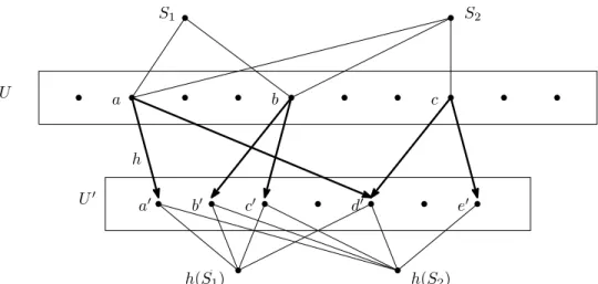
Figure 3.1: A diagram of reductions. We simplify this picture, and make the reductions to Edit Distance, LCS, etc. more meaningful. . . 36 Figure 3.2: The universe-shrinking process. S1 ={a,b} and S2 ={a,b,c}. After the

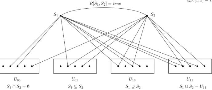
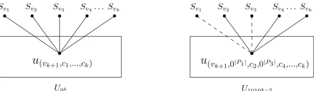
mappingh, the new sets areh(S1) =_{a0,b0,c0,d0_}andh(S2) =_{a0,b0,c0,d0,e0_}. 52 Figure 3.3: An example of a solution to a Hybrid Problem instance, whenk=2. . . 54 Figure 3.4: The formula is satisfied iff there exists(S_v1,S_v2, . . . ,S_vk)so that there does not

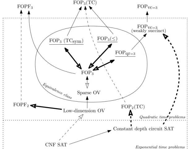
exist such an elementuin any of the sub-universes. . . 59 Figure 4.1: The expressive power and complexity of problems and classes of problems. . . 89

LIST OF TABLES

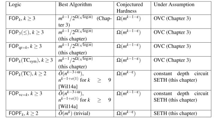
Table 3.1: Atomic Problems . . . 77 Table 4.1: Best algorithms and conjectured hardness of different classes of logic. . . 88

ACKNOWLEDGEMENTS

First of all I would like to thank my advisor Prof. Russell Impagliazzo for his invaluable help all these years. I would also like to thank Prof. Ramamohan Paturi for his help on all our projects. I would also like to acknowledge our co-authors Antonina Kolokolova, Ryan Williams, Marco Carmosino, Ivan Mihajlin, Stefan Schneider. I am glad that I took Prof. Victor Vianu’s database theory class, which raised my interest in first-order logic and model checking. I would also like to thank theory group students Anant Dhayal, Sasank Mouli, Jessica Sorrell and Jiapeng Zhang for helpful discussions about different problems. I am also thankful to my husband Jian Yang who gave me lots of support through this program. Finally I would like to thank coffee and diet coke.

Chapter 2 contains material from “Nondeterministic Extensions of the Strong Exponential Time Hypothesis and Consequences for Non-Reducibility”, by Marco L Carmosino, Jiawei Gao, Russell Impagliazzo, Ivan Mihajlin, Ramamohan Paturi, and Stefan Schneider, which appeared in the proceedings of the 2016 ACM Conference on Innovations in Theoretical Computer Science (ITCS 2016). The author of this dissertation was a principal author of this publication. The material in this chapter is copyright c2016 by Association for Computing Machinery. We would like to thank Amir Abboud, Karl Bringmann, Bart Jansen, Sebastian Krinninger, Virginia Vassilevska Williams, Ryan Williams and the anonymous reviewers for many helpful comments on an earlier draft.

Chapter 3 contains material from “Completeness for First-Order Properties on Sparse Struc-tures with Algorithmic Applications”, by Jiawei Gao, Russell Impagliazzo, Antonina Kolokolova, and Ryan Williams, which appeared in the proceedings of the Twenty-Eighth Annual ACM-SIAM Symposium on Discrete Algorithms (SODA 2017). The author of this dissertation was a principal author of this publication. The material in this chapter is copyright c2017 by Association for Computing Machinery and Society for Industrial and Applied Mathematics. We would thank Virginia Vassilevska Williams for her inspiring ideas. We would like to thank Marco Carmosino, Anant Dhayal, Ivan Mihajlin and Victor Vianu for proofreading and suggestions on this paper. We

also thank Valentine Kabanets, Ramamohan Paturi, Ramyaa Ramyaa and Stefan Schneider for many useful discussions. Finally, we really appreciate the suggestions from the reviewers about the writing and expression.

Chapter 4 contains material from “The Fine-Grained Complexity of Strengthenings of First-Order Logic”, by Jiawei Gao and Russell Impagliazzo, which is currently in submission. The author of this dissertation was a principal author of this work. The authors sincerely thank Marco Carmosino and Antonina Kolokolova for comments on improving this paper.

Chapter 5 contains material from “On the Fine-grained Complexity of Least Weight Sub-sequence in Multitrees and Bounded Treewidth DAGs”, by Jiawei Gao, to appear in International Symposium on Parameterized and Exact Computation (IPEC 2019). The author of this dissertation was a principal author of this publication. The author would like to thank Russell Impagliazzo for his guidance and advice on this paper, and thank Marco Carmosino, Anant Dhayal and Jessica Sorrell for helpful comments.

VITA

2013 B. E. in Software Engineering, Fudan University, Shanghai, China 2019 Ph. D. in Computer Science, University of California, San Diego

ABSTRACT OF THE DISSERTATION

The Fine-Grained Complexity of Problems Expressible by First-Order Logic and Its Extensions

by

Jiawei Gao

Doctor of Philosophy in Computer Science

University of California San Diego, 2019

Professor Russell Impagliazzo, Chair

This dissertation studies the fine-grained complexity of model checking problems for fixed logical formulas on sparse input structures.

The Orthogonal Vectors problem is an important and well-studied problem in fine-grained complexity: its hardness is implied by the Strong Exponential Time Hypothesis, and its hardness implies the hardness of many other interesting problems. We show that the Orthogonal Vectors problem is complete in the class of first-order model checking on sparse structures, under fine-grained reductions. In other words, the hardness of Orthogonal Vectors and the hardness of first-order model checking imply each other. This also gives us an improved algorithm for first-order model checking problems.

Among all first-order logic formulas in prenex normal form, we have reasons to believe that quantifier structures_∃. . ._∃∀and _∀. . ._∀∃may be the hardest in computational complexity: If the Nondeterministic version of the Strong Exponential Time Hypothesis is true, formulas of these forms are the only hard ones under the Strong Exponential Time Hypothesis.

We can add extensions to first-order logic to strengthen its expressive power. This work also studies the fine-grained complexity of first-order formulas with comparison on structures with total order, first-order formulas with transitive closure operations, first-order formulas of fixed quantifier rank, and first-order formulas of fixed variable complexity.

We also introduce a technique that can be used to reduce from sequential problems on graphs to parallel problems on sets, which can be applied to extending the Least Weight Subsequence problems from linear structures to some special classes of graphs.

Chapter 1

Introduction

1.1

Fine-Grained Complexity of Model Checking Problems

This dissertation presents results about the fine-grained complexity and algorithms about problems in polynomial time, that are describable by first-order logic or extensions of first-order logic. Fine-grained complexityis a relatively new sub-area within theoretical computer science that not only qualitatively classifies problems as “easy” or “hard”, but (to the extent possible) pin-points their exact complexities. It aims to make complexity theory more relevant to algorithm design (and vice versa) by giving reductions that better preserve the times required for solving problems, and connecting algorithmic progress with complexity theory. While some of the key ideas can be traced back to parameterized algorithms and complexity ([FJ56, DF92]), studies of the exact complexity of NP-complete problems ([SHI90, IPZ98, JS99, IP99]), and algorithmic consequences of circuit lower bounds ([AW85, Yao82, LMN93, NW94, BFNW93, IKW02, KI04]), the full power of this approach has emerged only recently. This approach has given us new circuit lower bounds ([Wil13, Wil14b]), surprising algorithmic improvements using circuit lower bound techniques ([AWY15, Wil05, CW16, CIKK16]), and many new insights into the relative difficulty of substantially improving known algorithms for a variety of problems both within and beyond polynomial time.

There are now a wide variety of standard algorithmic problems where no significant improvements in algorithmic running time can be made without refuting one of a few conjec-tures about well-studied problems, such as thek-SUM problem [GO95], All Pairs Shortest Paths [WW10, AGW14, LWW18], SAT, or Orthogonal Vectors [AWW14, BI15, BCH16, Bri14, ABW15, BI15, BK15, AHWW16, MPS16, KPS17, AR18, ABDN18, BRS+18]. As the field has grown, many fundamental relationships between problems have been discovered, making the graph of known results a somewhat tangled web of reductions.

Traditionally, complexity theory has been used to distinguish very hard problems, such as NP-complete problems, from relatively easy problems, such as those inP. However, over the past few decades, there has been progress in understanding the exact complexities of problems, both for very hard problems and those withinP, under plausible assumptions.

Unfortunately, as our understanding of the relationship between the exact complexities of problems grows, so does the complexity of the web of known reductions and the number of distinct conjectures these results are based on. Ideally, we would like to show that many of these conjectures are in fact equivalent, or that all follow from some basic unifying hypothesis, thereby improving our understanding and simplifying the state of knowledge. For example, it would be nice to show that the 3-SUMconjecture or the APSP conjecture follows from SETH. A result like that would reduce the number of conjectures we rely on to explain the complexity of problems.

At the same time, many problems seem to be hard, but their hardness is not explained by any of the three most popular conjectures in fine-grained complexity, SETH, the 3-SUMconjecture and the APSP conjecture. Among these questions is ifHITTINGSETcan be solved in subquadratic time or if MAXFLOWhas a linear time algorithm. For neither of these problems can we answer the question positively with an algorithm nor negatively with a conditional lower bound.

In traditional complexity, classes of problems are related to each other, and individual problems understood by identifying classes for which they are complete. In contrast, most of the results in fine-grained complexity were obtained on a problem-by-problem basis. One reason for this is that results in fine-grained complexity cut across traditional classes, withNP-complete

problems reducing to problems withinPor even smaller classes. This raises the questions: is it possible to give a fine-grained complexity of classes of problems? Is the notion of completeness useful in fine-grained complexity?

We study the class of problems where each problem asks whether the input structure satisfies a fixed first-order formula. This class is natural both in terms of computational complexity, where it is the uniform version ofAC₀, and in database theory, because these are the queries expressible in basic SQL [AHV95]. First-order logic can also express many polynomial time computable problems: ORTHOGONALVECTORS,k-ORTHOGONALVECTORS,k-CLIQUE,k-INDEPENDENTSET, k-DOMINATINGSET, etc. Not only were the likely complexities of the hardest problems (as a function of number of quantifiers) given, but in the second paper, a natural complete problem was identified, the orthogonal vectors problem (discussed below in more detail). The conclusion was that there were substantial improvements possible in the worst-case complexity of model checking for first-order properties if and only if the known Orthogonal Vectors algorithms can be substantially improved. Using a recent sub-polynomial improvement in OV algorithms by [AWY15], they obtained a similar improvement in model checking every first-order property.

In CNF-SAT problem, given a Boolean formulaF in CNF form (conjunction of disjunctions of (possibly negated) variables), the goal is to determine whether there is an assignment of Boolean values to variables ofF which makesF true. Ink-CNF-SAT, every clause (disjunction) can have at mostkliterals. We refer to the following conjecture about complexity of solving CNF-SAT:

Strong Exponential Time Hypothesis (SETH)1: For everyε>0, there exists ak≥2 so

thatk-CNF-SAT cannot be solved in timeO(2n(1−ε)_).

The problem of deciding whether a structure satisfies a logical formula is called the model checking problem. It is well-studied in finite model theory. In relational databases, first-order model checking plays an important role, as first-order queries capture the expressibility of relational algebra. In contrast to the combined complexity, where the database and query are both given

as input, thedata complexitymeasures the running time when the query is fixed. The combined complexity of first-order queries isPSPACE-complete, but the data complexity is inLOGSPACE [Var82]. Moreover, these problems are also major topics in parameterized complexity theory. In [FG06], Flum and Grohe organize parameterized first-order model-checking problems (many of which are graph problems) into hierarchical classes based on their quantifier structures. Here, we study model checking from the fine-grained complexity perspective.

This dissertation talks about model checking problem where the logical formula (i.e., the query) is fixed by the problem. We use the term “first-order property” to refer to these problems.

First-order properties are also extensively studied in complexity, logic (especially finite model theory and theory of databases) and combinatorics. For example, the first zero-one law for random graphs was proved for first-order properties on finite models ([Fag76]), and Ajtai’s lower bound forAC0[Ajt83] (proved independently by Furst, Saxe, and Sipser ([FSS84])) was motivated and stated as a result about inexpressibility in first-order logic.

There are many problems within P that are known to be SETH-hard, but few of them are first order property problems. And of the ones that are, they tend to have similar logical forms. For instance,k-DOMINATINGSET[BCH16] is definable by a_∀k_∃quantified formula; the GRAPHDIAMETER-2problem and the BIPARTITEGRAPHDOMINATEDVERTEXproblem [BCH16] are definable by_∀∀∃quantified formulas. Here we study the relations between SETH-hardness and the logical structures of model checking problems. A result by Ryan Williams [Wil14a] explored the first-order graph properties on dense graphs, while here we look into sparse graphs whose input is a list of edges.

We define first-order properties on hypergraphs. The input is a many-sorted universe that we view as sets of vertices, together with a number of unary relations (node colors), and binary relations, viewed as different categories or colors of edges. The binary relations are not symmetric in general. We specify the problem to be solved by a first order sentence. Let ϕbe a first order

sentence in prenex normal form, withkquantifiers:

ϕ=Q1x1∈X1,Q2x2∈X2, . . .Qkxk∈Xkψ (1.1)

or shortened as

ϕ=Q1x1Q2x2. . .Qkxkψ (1.2)

whereϕis a quantifier-free formula whose atoms are unary or binary predicates onx1, . . . ,xk.

An instance of the model checking problem of a formulaϕwithk≥3 quantifiers specifies

setsX1, . . .Xk, where variablexiis an element of setXi, as well as all the unary and binary relations

that occur inϕ. We assume without loss of generality that the setsXiare disjoint and that the domain

of any predicate is restricted to one pair(X_i,X_j). We can always duplicate elements and adjust the corresponding relations accordingly. We also assume equality is one of the relations, so we can tell whenx_i=x_j. To reformulate the problem as a graph problem, we view the setsX₁, . . . ,X_k as the sets of nodes in ak-partite graph, and the binary predicates as (colored) edges, i.e. for some predicateP, ifP(xi,xj)is true then there is an edge between the nodesxi andxj. We refer to the

k-partite graph with edges defined by predicatePasGP, and the colored union of graphs defined on

all predicates asG.

We assume that the input is given as follows: For each unary relation, we are given a Boolean vector indexed by the vertices saying whether the relation holds, and for each binary predicate, the list representation of the corresponding directed graph. We want to decide ifϕis true for the input

model.

Examples of this problem includek-CLIQUE, which is defined by

ϕ=∃x1. . .∃xk

^

i,j∈{1,...,k},i6=j

k-DOMINATINGSET, defined by

ϕ=∃x1. . .∃xk∀xk+1(E(x1,xk+1)∨ ··· ∨E(xk,xk+1)) (1.4)

and GRAPHRADIUS2, defined by

ϕ=∃x1∀x2∃x3(E(x1,x3)∧E(x3,x2)) (1.5)

We letn=maxi|Xi|be the maximum size of the node parts, andmbe the number of edges

in the union of the graphs. The size isn+m, but for convenience, we will assumem>nand usem as the input size.

1.2

Overview of the Dissertation

Section 1.3 gives the definitions of problems and classes used in this dissertation. Section 1.5 introduces the basic concepts and techniques of fine-grained complexity.

In Chapter 2, we introduce a new technique that provides reasons to believe that some problems may be strictly harder than some other problems. We show that under the Nondeterministic Strong Exponential Hypothesis, the hardest first-order property problems all have similar quantifier structures: either_∃. . .∃∀, or_∀. . .∀∃.

In Chapter 3, we prove that the well-studied Orthogonal Vectors problem is complete in the class of first-order property problems. In other words, improved algorithms for OV will imply better algorithms for all first-order property problems. This result shows that Orthogonal Vectors is a relatively hard problem. Even if the Strong Exponential Time Hypothesis is false, OV may remain hard if there exists a hard first-order property.

We give algorithms for every first-order property problem that improves this upper bound to mk/2Θ(√logn)_{, i.e., an improvement by a factor more than any poly-log, but less than the polynomial}

algorithms for sparse instances of the well-studied Orthogonal Vectors problem. Surprisingly, both results are obtained by showing completeness of the Sparse Orthogonal Vectors problem for the class of first-order properties under fine-grained reductions. To obtain improved algorithms, we apply the fast Orthogonal Vectors algorithm of [AWY15, CW16].

While fine-grained reductions (reductions that closely preserve the conjectured complexities of problems) have been used to relate the hardness of disparate specific problems both withinPand beyond, this is the first such completeness result for a standard complexity class.

Chapter 4 studies extensions of the class of first-order model checking problems, and studies this class with more lenient parameterizations. We consider classes obtained by allowing function symbols; first-order on ordered structures; adding various notions of transitive closure operations; and stratifications of first-order properties by quantifier depth and variable complexity, rather than number of quantifiers. For some of these classes, OV is still a complete problem, in that significant improvement for the entire class is equivalent to significant improvement for OV algorithms. For these classes, we can also use the improved OV algorithm of [AWY15, CW16] to get moderate improvements on algorithms for the entire class. For other classes, we show that model checking becomes harder than for first-order, under well-studied conjectures such as SETH. For these classes, we show hardness follows from weaker assumptions than SETH.

Surprisingly, whether an extension increases the complexity of model checking seems independent of whether it increases the expressive power of the logic. For example, adding function symbols does not change which problems are expressible by first-order, but does increase the time for model checking under SETH. On the other hand, adding an ordering does not change the fine-grained complexity of model checking, although it increases the logic’s expressive power.

Chapter 5 introduces a new technique that generalizes previously known subquadratic time reductions from linear structures to graphs. Least Weight Subsequence (LWS) is a class of highly sequential optimization problems with formF(j) =mini<j[F(i) +ci,j][HL87]. They can be solved

in quadratic time using dynamic programming, but it is not known whether these problems can be solved faster thann2−o(1)time. Surprisingly, each such problem is subquadratic time reducible to a

highly parallel, non-dynamic programming problem [KPS17]. In other words, if a “static” problem is faster than quadratic time, so is an LWS problem. For many instances of LWS, the sequential versions are equivalent to their static versions by subquadratic time reductions. The previous result applies to LWS on linear structures, and this chapter extends this result to LWS on paths in sparse graphs, the Least Weight Subpath (LWSP) problems. When the graph is a multitree (i.e. a DAG where any pair of vertices can have at most one path) or when the graph is a DAG whose underlying undirected graph has constant treewidth, we show that LWS on this graph is still subquadratically reducible to their corresponding static problems. For many instances, the graph versions are still equivalent to their static versions.

Moreover, this chapter shows that on these graphs, if we can decide a first-order property

∃x_∃yP(x,y)in subquadratic time, where Pis a quickly checkable property, then we can also in subquadratic time decide whether there are pairsx,yin the transitive closure of a DAG of the above types that satisfyP(x,y), which is a considerably more expressive class of problems.

Appendix A lists some example problems in the classes of problems studied in this disserta-tion.

1.3

Definitions of Model Checking Problems and Classes

1.4

First-Order Property Problems

Next we will give the definitions and notations regarding the model checking problems. Letϕbe a fixed formula and let Gbe an input structure, the model checking problem for ϕis to decide whetherGsatisfiesϕ. Whenϕis a first-order formula, we also call it a first-order

property problem.

ϕis a fixed formula without free variables (i.e. all variables are quantified by either∃or∀).

We use MCϕto denote the model checking problem for formulaϕ. In this dissertation we usually

LetterQis used to represent a quantifier, either_∃or_∀.

The input structure has multiple variable domains and multiple relations. It can be considered as a hypergraph (represented by adjacency list): the elements of the structure correspond to vertices, and the relation tuples of the structure correspond to edges.

Thedomain of a variableis a fixed set of vertices so that a variable inϕcan be assigned to

any one of the vertices. The total number of vertices isn.

Arelationis a fixed set of edges (or hyperedges) so that a binary (ort-ary) predicate inϕ

can correspond to one of the edges. The total number of edges ism. We only consider the case that m_≥n.

Because the number of edges is important in describing problem size, in the rest of this dissertation we define thedegreeof a vertexvto stand for the total number of edges the vertex is in.

let ϕbe a fixed first-order sentence containing free predicates of arbitrary constant arity

(and no other free variables). For example, the k-Orthogonal Vectors (k-OV) problem can be expressed by a (k+1)-quantifier formulaϕ= (∃v1 ∈A1). . .(∃vk ∈Ak)(∀i)

h

Wk

j=1¬(vj[i] =1)

i

. The model-checking problem forϕ, denoted byMCϕ, is deciding whetherϕis true on a given input

structure interpreting predicates inϕ(e.g., givenk sets of vectors, decidek-OV). We sometimes

refer to structures as “hypergraphs” (“graphs” when all relations are unary or binary), and relations as edges or hyperedges. We usento denote size of the universe of the structure andmthe total number of tuples in all its relations (size of the structure). Many graph properties such ask-clique have natural first-order representations, and set problems such as Hitting Set are representable in first-order logic using a relationR(u,S)≡(u_∈S).

We propose the following conjecture on the hardness of model checking of first-order properties.

First-order property conjecture (FOPC): There is an integer k_≥2, so that there is a

(k+1)-quantifier first-order property that cannot be decided inO(mk−ε_{)time, for any} ε>0.

Assumptions

˜

Onotation is generally used for time complexity hiding sub-polynomial time factors. But in this dissertation we usually consider savings factors in running time that grow faster than polylogarithmic, so we still use the big-O notation but let it hide polylogarithmic factors.

In this dissertation, without loss of generality we make the following assumptions.

• Assumem=n1+o(1), because otherwise theO(mnk−2)time baseline algorithm (Lemma 4.9.1) is better than the conjectured timemk−o(1).

• Assume that different variables are in different domains. (For instance, the universe ofxis X, the universe ofyisY, etc.) In other words, a structure for ak-quantifier formula can be considered as ak-partite graph. However, in the case where transitive closure operations can be taken on a relation, we will assume both variables of the relation are in the same universe.

• We assume that for any tuple of elements, the value of a predicate on this tuple can be queried in constant time. Also, assume that the neighbors of any elementvcan be enumerated in time linear to the degree ofv.

LetR₁, . . . ,R_r be predicates of constant aritiesa₁, . . . ,a_r(a vocabulary). A finitestructure over the vocabularyR₁, . . . ,R_r consists of auniverse U of sizentogether withrlists, one for every R_i, ofm_ituples of elements fromU on whichR_iholds. Letm=∑r_i=1mi; viewing the structure as a

database,mis the total number of records in all tables (relations).

We loosely use the termhypergraphto denote an arbitrary structure; in this case, we refer to its universe as a set of verticesV =_{v₁, . . . ,v_n}and call tuples(v₁, . . . ,v_ai)such thatR_i(v₁, . . . ,v_ai)

holds hyperedges (labeledR_i). A set of allR_i-labeled hyperedges in a given hypergraph is denoted byE_Ri or justE_i; the structure is denoted byG= (V,E₁, . . . ,E_r). Similarly, we use the termgraph for structures with only unary and binary relations (edges); here, we mean edge-labeled vertex-labeled directed graphs with possible self-loops, as we allow multiple binary and unary relations and relations do not have to be symmetric. This allows us to use graph terminology such as adegree (the number of (hyper)edges containing a given vertex) or a neighbourhood of a vertex.

Letϕbe a first-order sentence (i.e. formula without free first-order variables) containing

in prenex form. Themodel-checking problemfor afirst-order propertyϕ,MCϕ, is: given a structure

(hypergraph)G, determine whetherϕholds onG(denoted byG|=ϕ). We use notationFOPkfor the

class of model checking fork-quantifier first-order formulas in prenex form, andMC(Q1. . .Qk)for

the model checking for first-order prenex formulas with quantifier prefixQ1. . .Qk, with a shortcut

Qc_i denotingcconsecutive occurrences ofQ(e.g. MC(∃k_∀)).

We assume that (hyper)graphs are given as a list ofm(hyper)edges, with each hyperedge encoded by listing its elements. In the Word RAM model withO(logn)bit words, the size of an encoding of a hypergraph isO(n+m)words, and an algorithm can access a hyperedge in constant time. With additionalO(m)time preprocessing, we can compute degrees and lists of incident edges for each vertex, and store them in a hash table for a constant-time look-up; edges incident to a vertex can then be listed in time proportional to its degree. We also assume thatm_≥n, with every vertex incident to some edge, because the interesting instances are in this case. Moreover, we assume the (hyper)graph isk-partite wherekis the number of variables inϕ, so that each variable is selected

from a distinct vertex set. From any (hyper)graph, the construction of thisk-partite graph needs a linear time, linear space blowup preprocessing which creates at mostkduplicates of the vertices andk2duplicates of the edges. Finally, we treat domains of quantifiers as disjoint sets forming a partition of the universe; any structure can be converted into this form with constant increase of the universe size. We also view predicates on different variable sets (e.g.,R(x1,x2)vs. R(x2,x4)

vs.R(x₄,x4)) as different predicates, and partition corresponding edge sets appropriately.

The focus of this dissertation is onsparsestructures, that is, the case whenm_≤O(n1+γ_)for

someγsuch that 0≤γ<1. In particular, allEiare sparse relations; we use the termco-sparseto

refer to complements of sparse relations. We will usually measure complexity as a function ofm. From the following baseline algorithm which will be proved in Section 3.9.1, the sparse assumption is without loss of generality.

1.4.1

Types of First-Order Property Problems with Different Complexity

Measures

k-Quantifier Problems: Hereϕhas formQ1x1. . .Qkxkψ(x1, . . . ,xk). Without loss of

gener-ality, we assumeϕis in prenex normal form. For example, the sparse OV problem can be represented

by

ϕOV =∃x∃y∀z(¬One(x,z)∨ ¬One(y,z)),

wherex,yare vectors andzis a coordinate of the vectors.One(x,z)is true iff a vectorxhas a one on itsz-th coordinate. The sparsek-OV problem is equivalent to

ϕk−OV =∃x1. . .∃xk∀zWki=1(¬One(xk,z)).

We use the notation FOPk for the class of MCϕ where ϕ is a first-order formula with k

quantifiers. This is the class of problems studied in Chapter 3.

Quantifier Rank k Problems: The quantifier rank of a formula is the maximum depth of nesting of its quantifiers. When we can reuse the same variable name in different scopes, for example,

ϕ=∃x(∃y(∃zψ1∧ ∀zψ2)∧ ∀y(∃zψ3∨ ∀zψ4))

has only three variable names x,y,z, but they represent different variables in different scopes of the formula. The above formula is of quantifier rank 3. The property that graph verticess,t has a path of length`can be represented by a formula with`−1 existential quantifiers, but using the technique of Savitch’s Theorem, the quantifier rank can be only log`.

We use the notationFOP_qr=kfor the class ofMC_ϕ whereϕis a FO formula with quantifier

rankk. FOPqr=kcontainsFOPk. It can be solved in timeO(mnk−2)for anyk≥2 (Lemma 4.9.1).

This dissertation shows that, even though a formula with quantifier rankkmay have more thankvariables when converted to prenex normal form, but the following theorem shows that even if it seems more powerful, it is reducible to quantifier numberkproblems.

This theorem will be proved in Appendix 4.3.

Variable ComplexitykProblems: If we do not bound the quantifier rank ofϕ, it will have

even more expressive power, for example, a formula of form

ϕ=∃x∃y(R(x,y)∧ ∃x(R(y,x)∧ ∃y∃x(R(x,y)∧. . .)))

can represent a path of any constant length using only 2 variables.

A formula with k different variable names is referred to as ofvariable complexity k. A formula is of variable complexitykiff it can be computed by a straightline program, each line has at mostkdistinct variables (even if written in prenex form). That is, it’s equivalent to the result of a sequence of first-order queries of formR_i=_{(x1, . . . ,xa)|ϕi(x1, . . . ,xa)}where eachRiis an

intermediate relation of arity a(0_≤a_≤k), and each ϕi is a first-order formula with at most k

variables, includingx1, . . . ,xa, which appear as free variables inϕi.

When the variable complexity is 3, if in each line of the corresponding straightline program

ϕ, there is at most one occurrence of an intermediate binary relation computed in a previous line,

thenϕcan be solved inO(mn)time for sparse graphs, which will be shown in Appendix 4.10. In

this case we call this variable complexity 3 problemweakly succinct. Appendix 4.10 gives another example which is in matrix multiplication time but not known to haveO(mn)algorithms.

We use the notationFOP_vc=k for the class ofMC_ϕ whereϕis a FO formula with variable

complexityk. The class of weakly succinct problems inFOP_vc=k containsFOP_qr=k(Each line of the straightline program creates a new intermediate relation onx,yby an intermediate relation on x,yand some original relations on somez. We will not elaborate the details here).

The following theorem shows that the SETH of constant depth circuit implies the quadratic-time hardness ofFOPvc=3.

1.4.2

Types of Problems Definable by Extensions of First-Order Logic

k-Quantifier with Function Symbols: In first-order formulas, sometimes we allow a list of functions symbols f₁, . . . ,f_c. Here we only consider unary function symbols, because the description

of higher arity functions takesn2space in the input. To simulate higher arities, we could increase the universe to a Cartesian power and then have unary functions on this product space. Each function symbol fi maps an element to another element. Predicates can be taken on function symbols,

e.g.P(f1(x),f2(y)).

For example, the problem “checking if a graph coloring satisfies the condition that no pairs of vertices of distance 2 have the same coloring” can be written as_∀x_∀y(∃z(E(x,z)∧E(z,y))→

Diff(c(x),c(y))), where function c(x)maps vertex x to a colorc, and predicate Diff means two colors are different.

We use the notationFOPF_kfor the class ofMC_ϕ whereϕis ak-quantifier FO formula with

function symbols.

While we can simulate any function by a relation coding the graph of the function,Rf(x,y)

⇐⇒ f(x) =y, to express, for example that f(x1) = f(x2)we would need to write_∃y,R_f(x₁,y)_∧

R_f(x₂,y). So the number of quantifiers in the translated forumlas would increase, possibly up to the number of function symbols appearing in the original. However, there is still a trivial O(nk)algorithm for model checking ak-quantifier formula with functions. So, assuming the OV Conjecture, the complexity grows by at most a linear amount over that for first-order without functions.

We show that this increase is necessary. Compared to the linear time baseline algorithm for the model checking of 2 quantifier formulas, when we introduce function symbols, a 2 quantifier formula may require quadratic time to solve.

First-Order on Ordered Structures: If all the elements in the domain of some variable have a total order so that for any two elements a,b it may be a>b, a<b or a=b, then the comparison relation on two elements is a dense relation. But unlike general dense relations, it can be represented succinctly in the input byO(n)space.

An example is that we have a log of communications in a network with events where a processor receives or sends messages, and we want to verify that every message sent is later

received. This can be expressed by _∀e_∃e0((e<e0)_∧SameSender(e,e0)_∧SameReceiver(e,e0)_∧

SameMessage(e,e0)), whereeande0are two log entries.

We use the notationFOP_k(_≤)for the class ofMC_ϕwhereϕis ak-quantifier FO formula

with comparison predicates. FOP_k(_≤)containsFOP_k. It can be solved in timeO(mnk−2)for any k_≥2 (Lemma 4.9.1).

We will consider the case where elements are given a total pre-ordering, and there are three predicates expressing that an element is greater than, less than, or equivalent to another element in the ordering. The comparison relation is an implicit dense relation but can be represented in O(n)space in the input, by giving a table indexed by element, giving the element’s rank within the ordering, with equivalent elements given the same rank. (If we were not given this table, we could use any sorting algorithm to construct it inO(nlogn)time.) Using this table, we can list the elements by this ordering in timeO(n), and given any two elements, we can compare them in time O(1). The following theorem shows that adding comparison to first-order logic does not increase the fine-grained complexity because it is equivalent to first-order properties without comparison.

First-order with Transitive Closure: The transitive closure of a sparse relation may be a dense relation. The comparison relation is a special case, which is the transitive closure of the successor relation. We useTCR to denote the transitive closure of relationR.

OV can be expressed by a 2-quantifier formula with transitive closure operation: we connect each vectoruto each coordinateiiffOne(u,i), and connect each coordinateito each vectorviff One(v,i). Thenuis reachable toviffuis not orthogonal tov.

We use the notationFOPk(TC)for the class ofMCϕwhereϕis ak-quantifier FO formula

allowing transitive closure operations.FOPk(TC)containsFOPk(≤).

For the problems ofFOP_k(TC)where the transitive closure operations are only allowed on symmetric input relations, we use the notationFOP_k(TCsym)to donate the class of these problems.

Consider the model checking of a first-order formula with transitive closures, where the transitive closure operation can only be taken on symmetric input relations. In this caseTC_R(x,y)

is true iffxandyare in the same connected component by edges of undirected edge setR. Thus the formula can have binary predicates about whether two variables are in the same connected component or not. Note that there can be more than one symmetric relations that the transitive closure operation can be taken on. We we use the notationFOP_k(TCsym)to donate the class of these problems.

1.5

Fine-Grained Complexity Preliminaries

1.5.1

Fine-Grained Reductions

To establish the relationship between complexities of different problems, we use the notion of fine-grained reductionsas defined in [WW10]. Fine-grained reductions are defined with the motivation to control the exact complexity of the reducibility. For this purpose, we consider languages together with theirpresumed orconjecturedcomplexities. These reductions establish conditional hardness results of the form “If one problem has substantially faster algorithms, so does another problem”. We will also useexact complexity reductions(see definition 1.5.2), which strengthen the above claim to “if one problem has algorithms improved by a factor s(m), then another problem can be improved by a factorsc(m)” for some constantc. (Note that some fine-grained reductions already have this property.) The underlying computational model is the Word RAM withO(logn)bit words.

Thus, ifL2has an algorithm substantially faster thanT2,L1can be solved substantially faster

thanT1. 2

Below we give the formal definition of Fine-Grained Turing Reduction. 2_{In almost all fine-grained reductions,T}

1≥T2, that is, we usually reduce from harder problems to easier problems,

which may seem counter-intuitive. A harder problemL1can be reduced to a easier problemL2withT1>T2in two

ways: by making multiple calls to an algorithm solvingL2and/or by blowing up the size of theL2instance (e.g., the

reduction from CNF-SAT to OV [Wil05]). All reductions from higher complexity to lower complexity problems in this dissertation belong to the first type.

Actually, it is harder to fine-grained reduce from a problem with lower time complexity to a problem with higher time complexity (e.g., prove that(MC(k),mk−1)≤FGR(MC(k+1),mk)), because this direction often needs creating instances with size much smaller than the original instance size.

We use the pair(L,T)to denote a language together with its time complexityT. Intuitively, if(L1,T1)fine-grained reduces to(L2,T2), then any constant savings in the exponent of the time

complexity ofL2implies some constant savings in the exponent of the time complexity ofL1.

Definition 1.5.1(Fine-Grained Reductions (_≤FGR)). LetL1and L2be languages, and letT1 and

T₂be time bounds. We say that (L₁,T1)fine-grained reducesto(L₂,T2)(denoted(L₁,T1)≤FGR

(L₂,T2)) if for allε>0, there is aδ>0 and a deterministic Turing reduction

M

satisfying the following conditions.

(a) The time complexity of the Turing reduction without counting the oracle calls is bounded by T1−δ

1 .

TIME[

M

1 (1.6)

(b) Let ˜Q(

M

_M

∑

q_∈Q˜(M,x)

(T2(_|q_|))1−ε_≤(T1(n))1−δ

If a fine-grained reduction exists from(L₁,T1)to(L₂,T2), algorithmic savings forL₂ can be transferred toL₁. The definition gives us exactly what is needed to establish savings forL₁by simulating the machine

_M

2. The role of each parameter in the

definition of fine-grained reducibility makes this clear.

T₁: The presumed time to decideL₁, usually given by a trivial algorithm.

T2: The presumed time to decideL2.

ε: Any savings (assumed or real) on computingL2.

It is easy to verify that fine-grained reductions, just like polynomial time reductions, can be composed.

Lemma 1.5.1(Fine-grained reductions are closed under composition). Let(A,TA)≤FGR(B,TB)

and(B,T_B)_≤FGR(C,TC). It then follows(A,TA)≤FGR(C,TC).

To simplify transferring algorithmic results, we define a stricter variant of fine-grained reductions, which we callexact reductions. These reductions satisfy a stronger reducibility notion. Definition 1.5.2. (Exact complexity reduction (_≤EC))

LetL1andL2be languages and letT1,T2denote time bounds. Then(L1,T1)≤EC(L2,T2)if there

exists an algorithmAL1 forL1running in timeT1(n)on inputs of lengthn, making calls to oracle of

L2with query lengthsn1, . . . ,nq, whereqis the number of calls and∑_iq₌₁T2(ni)≤T1(n).

That is, ifL₂is solvable in timeT2(n), thenA_L1 solvesL₁in timeT1(n).

The same fine-grained reductions also transfer nondeterministic and co-nondeterministic savings. In particular, the existence of both a fast nondeterministic and co-nondeterministic algorithm forL₂implies that there are also fast nondeterministic and co-nondeterministic algorithms forL1.

Lemma 1.5.2(Fine-grained reductions transfer savings for(N_∩coN)TIME). Let (L1,T1)≤FGR

(L₂,T2), and L_2∈(N_∩coN)TIME[T2(n)1₋ε_{]for someε>0. Then there exists aδ>0such that}

L_1∈(N_∩coN)TIME[T1(n)1−δ_]

Proof. Both the nondeterministic algorithm forL1and¬L1follow the same outline. We simulate the

deterministic Turing reduction

_M

q_∈Q˜(

M

of the fine-grained reduction we haveTIME[

M

and henceL_1∈NTIME[T₁(n)1₋δ_{]. Similarly we haveL}

1∈coNTIME[T1(n)1−δ]as we can negate

the output of the fine-grained reduction

M

We define nondeterministic fine-grained reductions as follows.

Definition 1.5.3(Nondeterministic Fine-Grained Reductions). LetL1 andL2 be languages, and

let T1 and T2 be time bounds. We say that(L1,T1)nondeterministically fine-grained reduces to (L2,T2)if for allε>0, there is aδ>0 and two nondeterministic Turing reductions

M

M

satisfying the following conditions.

(a) For allx_∈L1, then there is aywith|y| ≤T₁1−δsuch that

M

(b) For allx_6∈L₁, then there is aywith_|y_{| ≤}T1−δ

1 such that

M

(c) The time complexity of both Turing reduction without counting the oracle calls is bounded by T1−δ

1 , that is, forc∈ {1,2}

TIME[

M

(d) Let ˜Q(

M

_M

∑

q∈_Q˜_(Mc,x)

(T2(_|q_|))1−ε_≤(T1(n))1−δ

To prove Lemma 1.5.2 under nondeterministic reductions we can nondeterministically guess yand simulate

M

M

forL1and6=L1.

1.5.2

Conjectures

The Orthogonal Vectors (OV) problem is a well-studied problem in the field of fine-grained complexity. Its hardness is implied by the hardness of CNF-SAT, and implies the hardness of many

problems (A list of hardness results under OV conjecture is compiled in [Wil18]). It is defined as follows: Given a setAofnBoolean vectors of dimensiond, and must decide if there areu,v_∈A such thatuandvare orthogonal, i.e.,u[i]_·v[i] =0 for all indicesi_{∈ {}1, . . . ,d_}. Another (equivalent) version is to decide with two setsAandBof Boolean vectors whether there areu_∈Aandv_∈Bso thatuand vare orthogonal. A na¨ıve algorithm for OV runs in timeO(n2d), and the best known algorithm runs inn2−Ω(1/log(d/logn)) _{[AWY15, CW16].}

In this dissertation we introduce a version of OV we call theSparse Orthogonal Vectors (Sparse OV) problem, where the input is a list of m vector-index pairs (v,i) for each v[i] =1 (corresponding to the adjacency list representation of graphs) and complexity is measured in terms ofm; we usually considerm=O(n1+γ_{) for some 0≤}

γ<1. The popular hardness conjectures on OV

restrict the dimensiondto be betweenω(logn)(low dimension) andno(1) (moderate dimension);

however in Sparse OV we do not restrictd.

We thus identify three versions of Orthogonal Vector Conjecture, based on the size of the dimensiond. In all three conjectures the complexity is measured in the word RAM model with O(logn)bit words.

Low-dimension OVC (LDOVC): For allε>0, there is noO(n2−ε)time algorithm for OV with

dimensiond=ω(logn).

Moderate-dimension OVC (MDOVC): For allε>0, there is noO(n2−εpoly(d))time algorithm

that solves OV with dimensiond.

Sparse OVC (SOVC): For allε>0, there is noO(m2−ε)time algorithm for Sparse OV wherem

is the total Hamming weight of input vectors.

OV can be extended to thek-OV problem for any integerk_≥2: givenksetsA1, . . . ,Ak of

Boolean vectors, determine if there arekdifferent vectorsv_1∈A₁, . . . ,v_k∈A_k so that for all indices i,∏kj=1vj[i] =0 (that is, their inner product is 0). We naturally define a sparse version ofk-OV

similar to Sparse OV, where all ones in the vectors are given in a list.

thatk-CNF-SAT cannot be solved in timeO(2n(1−ε)_{). [IPZ98]}

Strong Exponential Time Hypothesis(SETH) for circuit classC For allε>0, the satisfiability

ofCcannot be solved in timeO(2n(1−ε)_{). [AHWW16] For each depthd, the SETH for}

depth-dcircuit forms a hierarchy of hardness. It is analogous to the W-hierarchy in parameterized complexity theory [DF95].

Nondeterministic Strong Exponential Time Hypotheses For allε>0, there exists a k so that

k-SAT is not incoNTIME[2n(1−ε)_{]. [CGI}+_16]

Low-dimension OVC (LDOVC): For allε>0, there is noO(n2−ε)time algorithm for OV with

dimensiond=ω(logn).

Moderate-dimension OVC (MDOVC): For allε>0, there is noO(n2−εpoly(d))time algorithm

that solves OV with dimensiond. [GIKW17]

Sparse OVC (SOVC): For allε>0, there is noO(m2−ε)time algorithm for Sparse OV wherem

is the total Hamming weight of input vectors. [GIKW17]

First-order property conjecture (FOPC): There is an integer k _≥2, so that there is a (k+

1)-quantifier first-order property that cannot be decided in O(mk−ε_{) time, for any}

ε>0.

[GIKW17]

Hitting Set Conjecture _∀ε>0 there is no O(n2−ε) time algorithm for the Hitting Set problem

with set sizes bounded by d=ω(logn). It implies LDOVC; subquadratic approximation

algorithms for Diameter-2 and Radius-2 would respectively refute the LDOVC and the Hitting Set Conjecture. [AWW16]

It is known that SETH implies LDOVC[Wil05]. Because MDOVC is a weakening of LDOVC, it follows from the latter.3 Like LDOVC, MDOVC also implies the hardness of problems 3_{Although dimensiondis not restricted, we call it “moderate dimension” because such an algorithm only improves}

including Edit Distance, LCS, etc. Here we further show that MDOVC and SOVC are equivalent (see Lemma 3.1.1).

The SETH of CNF-SAT implies LDOVC [Wil05], and LDOVC implies MDOVC because low-dimension OV is a special case of moderate-dimension OV. MDOVC, SOVC and FOPC are equivalent [GI19] (Will be shown in Chapter 3). The SETH of depthdcircuits, wheredis a constant greater than 2, is weaker than the SETH of CNF-SAT.

1.5.3

Basic Reduction Techniques

Quantifier-Eliminating Self reduction

A useful reduction is that(FOP_k+1,n_·T(m,n))_≤EC(FOPk,T(m,n)), whereT(m,n)is the

running time onmedges andnvertices. This is because we can exhaustively search the outermost quantified variable, and use the value as a constant in the rest of the formula, thus reducing it ton instances of the model checking fork-quantifier formulas. The same technique can also be applied in the reductions for formulas with comparisons, and formulas of quantifier rankk.

Split and List

The “Split and List” technique was used in the reduction from CNF-SAT to Orthogonal Vectors.

Letϕbe a CNF withnvariables andmclauses. We partition the variables into two sets,

each of sizen/2. For each set, there are 2n/2possible assignments to then/2 variables. Create two setsA,B, each containing 2n/2 boolean vectors of lengthm. Each boolean vector corresponds to an assignment ton/2 variables. If an assignment does not satisfy thei-th clause, we let the i-th bit of the corresponding variable be 1, otherwise be 0. Thus, there exist assignmentαfor the first

half of the variables andβfor the second half of the variables that together satisfyingϕiff for all

clauses, eitherαsatisfies it orβsatisfies it, iff either the vectorvα∈Aorvβ∈Bhas a zero on all

coordinates, iffv_αandv_βare a pair of orthogonal vectors.

is in timeO(2n/22−ε) =O(2n(1−ε/2)_).

This technique will be used in reducing the satisfiability of constant depth circuits to model checking for formulas of variable complexity 3, in Chapter 2.

High-Degree Low-Degree Trick

The High-Degree Low Degree Trick is a commonly used trick. For example, it was used in proving Triangle Detection in sparse graphs is in timeO(m3/2).

We split the set of vertices into two parts: those with degree greater than√m, and those with degree less than√m.

For the vertices of degree greater than √m, there can be at most O(p(m))of them, for otherwise the total number of edges would exceedm. So inO(√m)time we can enumerate the high degree vertices, and then usingO(m)time to enumerating the opposite edge, we can find any triangle containing a large degree vertex.

For the small degree vertices, we useO(m)time to enumerate all edges containing such a vertice, and then useO(√m)time to enumerate all the neighbors of the current vertex to find the third point of the triangle, if there is one.

This technique will be used in the algorithm for_∃∃∃and_∀∃∃problems in Chapter 1, and the reduction algorithm for quantifier-rank 3 problems in Chapter 2.

Grouping reduction

Thegrouping-reduction techniqueis another useful reduction technique, which was intro-duced in [AWY15], that reduces the Batch OV problem to OV, and in [AWW16], that reduces Hitting Set to OV. In [GIKW17] it is used on the model checking on sparse structures. The reduction can be generalized to get the following statement: Assume the model checking forϕ=∃x1. . .∃xk

P(x₁, . . . ,x_k)can be decided in timeO(mk/s(m))for some savings factors, wherePis a property onx₁, . . . ,x_kthat can be decided in time linear to the total degree ofx₁, . . . ,x_k. Then we can list all xsuch that_∃x₂. . ._∃x_kP(x₁, . . . ,x_k)can be decided in timeO(mk/s(poly(m))).

elements of weight greater thang, we enumerate all of them, and for each of them we run aO(mk−1)

algorithm to decide ifPholds onxby doing exhaustive search on all other variables. So the total time isO(m/g)_·O(mk−1) =O(mk/g).

Next, partition each of the domain ofx1, . . . ,xk into groups so that a group has total weight

at most g, and there are O(m/g)groups for each of x₁, . . . ,x_k. Every time we take ak-tuple of groups, and query ϕon this smaller instance. As long as the query returns true, we can find a

satisfyingx₁in O(logg)queries. On finding a satisfyingx₁, we mark thisx₁ and remove thisx₁ from its group. Continue this process until either allx₁are marked or no combination of groups satisfiesϕ. There are at mostO(mlogg+ (m/g)k)calls to the oracle ofϕ. The running time is

O(mlogg_·m_·(m/g)k_·gk_{/s(g)) =O(logg·m}k_/s(g)).

Thus the final running time is O(mk/g+logg_·mk/s(g)). The logarithmic factor can be omitted if functionsgrows much faster than polylog functions.

Chapter 2

Consequences Under the Nondeterministic

Strong Exponential Time Hypothesis

2.1

Introducing

NSETH

The Strong Exponential Time Hypothesis conjectures thatk-CNF-SAT cannot be solved efficiently by a deterministic algorithm, which can be considered as a fine-grained version of P₆=NP. If k-CNF-SAT is not only hard to solve using deterministic algorithms, but also by co-nondeterministic algorithms, then we get a fine-grained version of P ₆=NP. This chapter introduces this new hardness conjecture, which we call theNondeterministic Strong Exponential Time Hypothesis(NSETH). If NSETH is true, the hardness of problems under different popular conjectures is unlikely to be unified.

If any problem inNP_∩coNPcan be shown to beNP-complete, thenNP=coNP. Hence, assumingNP₆=coNP, placing a problem LinNP_∩coNPmeans that Lcannot beNP-complete (orcoNP-complete) and there is no polynomial time reduction from anNP-complete problem like 3-SATtoL. Similarly, by considering the nondeterministic and co-nondeterministic complexities of problems on a more fine-grained level, we deduce non-reducibility results based on NSETH.

Definition 2.1.1 (Nondeterministic Strong Exponential Time Hypothesis (NSETH)). For every

ε>0, there exists akso thatk-SATis not incoNTIME[2n(1−ε)_].

Equivalently, the k-TAUT problem, the tautology problem on k-DNF formulas, is not in NTIME[2n(1−ε)_{]for sufficiently largek.}

We feel that NSETH is plausible for many of the same reasons as SETH. We can think of NSETH as a statement about proof systems. Just as many algorithmic techniques have been developed fork-SAT, all of which approach exhaustive search for large k, many proof systems have been considered for k-TAUT, and none have been shown to have significantly less than 2n complexity for largek. In fact, the tree-like ([PI00]) and regular resolution ([BI13]) proof systems have been proved to require such sizes. Moreover, we observe that results of [JMV15] that obtain circuit lower bounds assuming SETH is false yield the same bounds assuming that NSETH is false. So disproving NSETH would be both a breakthrough in proof complexity and in circuit complexity.

We also consider the natural nondeterministic variant of ETH.

Definition 2.1.2(Nondeterministic Exponential Time Hypothesis (ETH)). The 3-SATproblem on nvariables requires is not incoNTIME[2εn_{]for someε>0.}

In [CGI+16], we show non-reducibility results for the following problems and time bounds.

• HITTINGSETfor sets of total sizemand timeT(m) =m1+γ_{is not SETH-hard for anyγ>0,}

and no problem that is SETH-hard fine-grained reduces toHITTINGSET for any such time complexity.

• 3-SUMforT(n) =n1.5+γ_{is not SETH-hard for anyγ>0.}

• MAXFLOW, minimum cost MAXFLOW, and maximum cardinality matching on a graph with medges andT(m) =m1+γ_{are not SETH-hard.}

• APSP on a graph withnvertices andT(n) =n3+ω2 +γis not SETH-hard. All the results above are assuming NSETH and under deterministic reductions.

2.1.1

Reasons that

NSETH

Is Hard to Refute

SETH is an interesting hypothesis because both_¬SETH and SETH have interesting con-sequences that seem difficult to prove unconditionally. In this chapter, we show that the same proofs that show “_¬SETH implies circuit lower bounds” can be applied to_¬NSETH as well. This is evidence that NSETH will be hard to refute.

Algorithms for CKT-SAT or CKT-TAUT imply circuit lower bounds (see [Wil13] and [Wil14b]). For some restricted circuit classes

_C

C

_C

_C

The proofs of [JMV15] optimize the reduction of arbitrary nondeterministic time languages to 3-SATto obtain new “failure of a hardness hypothesis aboutk-SATimplies circuit lower bounds” results for a variety of circuit classes. The followin is implicit in their work:

Theorem 1. We have the following implications from failure of a k-TAUThardness hypothesis to circuit lower bounds for restricted classes:

1. If the nondeterministic exponential time hypothesis (NETH) is false; i.e., for every ε>0,

3-TAUTis in time2εn_{, then∃f ∈E}NP_{such that f does not have linear-size circuits.}

2. If the nondeterministic strong exponential time hypothesis (NSETH) is false; i.e., there is a

δ<1such that for every k, k-TAUTis in time2δn, then∃f ∈ENPsuch that f does not have linear-size series-parallel circuits.

3. If there isα>0such that nα-TAUTis in time2n−ω(n/log logn)_{, then∃f ∈E}NP_{such that f does} not have linear-size log-depth circuits.

The theorem is proved in the full version of [CGI+16]. Since (by item 2 above) refuting NSETH would give nontrivial circuit lower bounds, it is unlikely to be easy to refute.

2.1.2

Hardness of Reducibility under

NSETH

How could we show that one language is not reducible to another language? There is an ever-growing web of problems, hypotheses, and reductions that reflect the fine-grained complexity approach to explaining hardness. Could this structure collapse into a radically simpler graph, with just a few equivalence classes? If we assume NSETH, probably not as much as one might hope.

We can broadly categorize computational problems into two sets. In the first category, the deterministic time complexity is higher than both the nondeterministic and co-nondeterministic time complexity. In the second category, at least one of nondeterminism or co-nondeterminism does not help in solving the problem more efficiently. Lemma 1.5.2 shows that savings in(N_∩coN)TIMEare preserved under deterministic fine-grained reductions. As a result, we can rule out tight reductions from a problem that is hard using nondeterminism or co-nondeterminism to a problem that is easy in(N_∩coN)TIME.

If NSETH holds, then k-SAT is in the category of problems that do not benefit fron co-nondeterminism. So, any problem that is SETH-hard under deterministic reductions also falls into this category.

In this chapter we explore problems that do benefit from (N_∩coN)TIME, i.e. we give nondeterministic algorithms that are faster than their presumed deterministic time complexities. This rules out deterministic fine-grained reductions from CNFSAT to these problems with their presumed time complexities. As a consequence, it is not possible to show that these problems are SETH-hard using a deterministic reduction.

As an immediate consequence of Lemma 1.5.2 we get a way to show non-reducibility assuming NSETH.

Corollary 2.1.1. AssumingNSETH, for any problem L and time bound T , if L_∈(N_∩coN)TIME[T(n)1₋δ_]

While Lemma 1.5.2 and Corollary 2.1.1 are formulated with respect to deterministic fine-grained reductions, we can extend the result to nondeterministic and zero-error reductions. On the other hand, the results do not extend to randomized reductions.

Theorem 2(NSETH implies no reduction fromCNFSAT). IfNSETHand C∈(N∩coN)TIME[T] for some problem C and time T , then(CNFSAT,2n)6≤FGR(C,T1+γ)for anyγ>0.

Proof. Assume NSETH and(CNFSAT,2n)≤FGR(C,T1+γ), andC∈(N∩coN)TIME[T]. By Lemma

1.5.2, preservation of(N_∩coN)TIMEsavings under fine-grained reductions, there existsδ>0 such

thatCNFSAT∈(N∩coN)TIME[2n(1−δ)_{]. This contradicts NSETH, therefore it cannot be the case}

(under NSETH) that(SAT,2n)_≤FGR(C,T).

Corollary 2.1.2(NSETH implies no reductions from SETH-hard problems). IfNSETHholds and C_∈(N_∩coN)TIME[T1], then for any problem B that isSETH-hard under deterministic reductions with time T₂, andγ>0, we have

(B,T2)_6≤FGR(C,T₁1+γ)

Proof. Assume NSETH, and that(B,T2)is SETH-hard. Therefore, we know

(CNFSAT,2n)_≤FGR(B,T2) (2.1)

Now assume(B,T2)≤FGR(C,T₁1+γ). Then by Lemma 1.5.1, composition of fine-grained reductions,

we have that(CNFSAT,2n)≤FGR(C,T1). But by Lemma 2 above, this is impossible under NSETH.

We have the following theorem:

Theorem 3. UnderNSETH, there is no deterministic or zero-error fine-grained reduction from SATor anySETH-hard problem to the following problems with the following time complexities for anyγ>0.

• MAXFLOW, min-costMAXFLOW, and maximum matching with T(m) =m1+γ

• HITTINGSETwith T(m) =m1+γ

• 3-SUMwith T(n) =n1.5+γ

• All-pairs shortest path with T(n) =n3+ω2 +γ

The theorem is proved in the full version of [CGI+16].

2.2

Characterizing the Quantifier Structure of SETH-Hard FO

Property Problems

This section studies the hardness of first-order model checking problems with the same number of quantifiers but different quantifier structures. If NSETH holds, all such formulas that are SETH hard are of a specific logical form. This is made precise as follows:

Theorem 4. Let k_≥3. IfNSETHis true, then there is a problem inFOPk that is O(mk−1)SETH

-hard, and all such formulas have the quantifier structure_∀k−1_∃or_∃k−1_∀.

The rest of this section proves the above theorem for the case where there are only unary and binary predicates (i.e., the input structure is a graph, instead of a hypergraph, so the problem is also called afirst-order graph propertyproblem). In this section, we will always assume formulas havek-quantifiers, instead of(k+1)quantifiers.

There are graph properties with_∀k−1_∃and_∃k−1_∀quantifier structure that are SETH-hard for timeO(mk−1).

The(k₋1)-ORTHOGONALVECTORSproblem is equivalent to the graph problem

∃x1. . .∃xk−1∀xk(P(x1,xk)∧ ··· ∧P(xk−1,xk)) (2.2)