QoS Aware Query Processing Algorithm for
Wireless Sensor Networks
Jun-Zhao Sun Academy of Finland
Department of Electrical and Information Engineering, University of Oulu Email: [email protected]
Abstract—In sensor networks, continuous query is commonly used for collecting periodical data from the objects under monitoring. This sort of queries needs to be carefully designed, in order to minimize the power consumption and maximize the lifetime of the sensor nodes. Data reduction techniques can be employed to decrease the size and frequency of data to be transferred in the network, and therefore save energy. This paper presents a novel method for optimizing sliding window based continuous queries. In particular, we deal with two categories of aggregation operations: stepwise aggregation (e.g. MAX, MIN, SUM, COUNT, AVERAGE, etc.) and direct aggregation (e.g. MEDIAN). Our approach is, by using packet merging or compression techniques, to reduce the data size to the best extent, so that the total performance is optimal. A QoS weight item is specified together with a query, in which the importance of the four factors, power, delay, accuracy and error rate can be expressed. Then an optimal query plan can be obtained by studying all the factors simultaneously, leading to the minimum cost. System models for energy and time consumptions of communication are created. Problem is formalized and algorithm is described in detail. Finally, experiments are conducted to validate the effectiveness of the proposed method.
Index Terms—Sensor networks, Query processing, Data gathering, QoS, aggregation
I. INTRODUCTION
Sensor networks represent significant improvement over traditional sensors in many ways like large-scale, densely deployment, ad-hoc & self-organization, prone to failures, changing topology, and with limited in power, computational capacities. The concept of micro-sensing and wireless connection of sensor nodes promises many new application areas e.g. military, environment, health, home, to name a few [1, 2].
Sensor nodes have very limited supply of energy, and should be available in function for extremely long time (e.g. a couple of years) without being re-charged. Therefore, energy conservation needs to be one key consideration in the design of the system and applications. Extensive research work has been devoted to address the problem of energy conservation. Examples include energy efficient MAC protocol [3], clustering [4], localization [5], routing [6], data management [7], as well as applications [8].
At high level, a sensor network can be modelled by a database view. Continuous query is commonly used for collecting periodical data from the objects under monitoring. This query needs to be carefully designed, in order to minimize the power consumption and maximize the lifetime. Data reduction techniques like packet merging, data compression, and aggregation and fusion can be employed to decrease the size of data to be transferred in the network, and therefore save energy of sensor nodes.
This paper presents a novel method for the optimization of continuous query, and in particular, for the last stage of query processing: query result collection. The key novelty of the method lies on the careful consideration of QoS issue along with data gathering. By taking advantage of the QoS constraints on power, delay, accuracy, and error rate specified with a query, the method can find the optimal combination of transmitting sensor data to sink. Our contributions can be summarized as follows.
1) A query representation scheme is proposed, in which SQL based grammar is extended with sliding window, QoS constraint weight item, and sample clause.
2) A WSN system model is created to model power consumption and time cost for both computation (data processing) and communication (data transmission).
3) A novel method is proposed for the optimization of continuous query with stepwise aggregation (e.g. MAX, MIN, SUM, COUNT, AVERAGE, etc.). The method is described in detail including the determination of both sample rate and data integration.
4) A method is presented for the optimization of continuous query with direct aggregation (e.g. MEDIAN). The similarity and variation of the previous method are discussed.
II. QUERY IN SENSOR NETWORKS
This section presents a database view of sensor networks and proposes the components for query representation.
A. Sensor database and query
A sensor field is like a database with dynamic, distributed, and unreliable data across geographically dispersed nodes from the environment. These features render the database view [9-11] more challenging, particularly for applications with the low-latency, real-time, and high-reliability requirements.
Under a database view, a wireless sensor network is treated as a virtual relational table, with one column per attribute and one row per data entry. For example a virtual table may have the structure as follows.
< location, time, temperature, light, humidity >
Sensor network applications use queries to retrieve data from the networks. The result is a logical sub-table of the whole virtual table of the network, with each data entry an associated timestamp to denote the time of measurement. The real data table of a node is different from the one in the virtual table in the sense that there will be only one attribute there. Usually, one sensor network should allow multiple co-existing queries in execution simultaneously. Therefore, data should be attached with a query ID to distinguish the query results. An real data example in a sensor node is as follows.
< query ID, node ID, time, temperature >
Query processing is employed to retrieve sensor data from the network [12-14]. A general scenario of querying sensor network is, as shown in Figure 1, when user requires some information, he or she specifies queries through an interface at sink (also known as gateway, base station, etc.). Then, queries are parsed and query plans are made. After that, queries are injected into the network for dissemination. One query may eventually be distributed to only a small set of sensor nodes for processing. When sensor node has the sample data ready, results flow up out of the network to the sink. The data can then be stored for further analysis and/or visualized for end user.
Obviously, there are a couple of features that are
unique to query in sensor network comparing to normal database query. First, data in sensor network is not available when query is issued. Second, in sensor network query is often conducted over a stream of data varying in time, instead of static fixed-size data. Finally, data in sensor network is approximate instead of exact. New techniques are therefore needed in handling sensor network queries.
B. Query components
A query contains following elements:
1) Data attributes that are required by the applications, corresponding to the columns of the virtual table.
2) Operations on the collected data. Simple operations are those aggregation functions, including average, sum, max, min, and count. Complex operations can be defined as data fusion functions, and are mostly used for multimedia data. There can always be application-specific fusion functions defined.
3) Sensor selection predicate, which specifies the Boolean condition of when a particular data entry of a sensor in the virtual table will be selected as one record in the query result table. It is a logical expression with relevant data attributes as the operands, and returns true or false.
4) QoS constraints, which specify application’s QoS requirements on both the query execution and the resulted data. The constraints is utilized in the query plan and execution to compromise between quality and cost.
5) Trade-off between the quality of the data (accuracy, delay) and power cost, which defines the importance of factors involved in making a query plan. Different factors are assigned different weights to denote the importance of the corresponding factors from the observer’s point of view.
6) Temporal information, which specify the moment, interval, and times that data should be collected (i.e. sensor perform the measurement).
SQL-based query language, which consists of a SELECT-FROM-WHERE clause, representation is commonly accepted, and so widely used in specifying queries for sensor networks as well. However, sensor network has its own characteristics, and therefore extensions must be made to the basic SQL query. Query representation for sensor networks is out of the scope of this paper. Below are two simple examples query in the form of extended SQL.
// Example query 1
SELECT WINMEDIAN ( S.temperature, 10 min, 2 min)
AS MEDIANTEMP
FROM sensors AS S
WHERE S.location = Area_C WHILE delay < 10 min
AND accuracy > 0.9 AND error < 0.01
WEIGHT (power, time, accuracy, error) = (0.4, 0.1, 0.3, 0.2)
Sink
SAMPLE
ON Now + 5 min RATE min 100
//Example query 2
SELECT WINCOUNT(*, 10 min, 2 min)
FROM sensors AS S
WHERE S.location = Area_C AND S.temperature > 4 C WHILE delay < 10 min
AND accuracy > 0.9 AND error < 0.01
WEIGHT (power, time, accuracy, error) = (0.4, 0.1, 0.3, 0.2)
SAMPLE
ON 00:00:00 RATE min 100
These are two queries to be performed above streaming data by using a sliding window. In the first example, the query specifies that after 5 minutes from now, the sensors in Area_C should start to measure and report the median temperature of the past 10 minutes once per 2 minutes, until further command stop them, and the result median temperature should be reported within 10 minutes after the value is ready. Here, temperature is the interesting data attribute, sliding window median is the operation, location restriction serves as the sensor selection condition, delay in WHILE clause is as the QoS constraint, and the SAMPLE clause specifies the temporal information. In the second example, the query reports the number of times that the temperature is above 4 C within recent 30 minutes once every 10 minutes.
The WEIGHT clause gives the weights of the factors in the quality-cost trade-off, by which the query plan can be optimized. This is the key idea of this paper. In the two examples above, four factors are considered as the weight items, power consumption, report delay in time, and the accuracy and error rate of the result. The queries give the sample starting time by ON clause and a minimum sample interval by a RATE clause. The really interval for sampling should be decided by the tradeoff denoted as the WEIGHT clause.
This paper concentrates on the optimization of periodical aggregation queries during the fourth stage of query execution: result collection (see Figure 1). In
particular, we mainly consider the situation where there are both delay and accuracy constraints, a weight item, and aggregation operations of average and count to be performed over collected data in the query. These two sorts of queries are very popular in real world applications like environment monitoring and healthcare.
III. DATA REDUCTION TECHNIQUES
Data reduction is to decrease the size of data that is needed in the communication. The idea is straightforward: less amount of data consumes less amount of power in transmission. Various data reduction techniques exists in this context, including packet merging, packet compression, data aggregation, and data fusion. This paper studies the first two techniques: packet merging and packet compression.
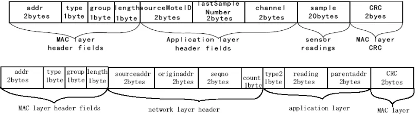
Packet merging is a simple data reduction technique, which combines multiple small packets into a big one, without considering the correlations between and the semantics within individual packets. In wireless communication, it is much expensive to send multiple smaller packets instead of one larger packet. One packet contains two parts, header and payload. Packet header is the packet overhead whose format is common for all the packet, which contains numbering, addressing and error checking information. The packet formats for sensor report streams in two representative applications provided by TinyOS, OscilloscopeRF and Surge, are shown in Figure 2 [15].
This commonly used packet structure forms the basis of packet merging – multiple packet can be combined so that only one packet header is presented with the rest the combination of the payloads of all the packets.
Packet compression is to integrate one or multiple packets into a reduced packet, by employing suitable data compression algorithms. A number of compression algorithms have been studied for sensor networks. According to the experimental results in [16-18], for most compression algorithms, compressing data before transmission reduces total power consumed. However, in some cases applying data compression increases total power consumption. This is due to accessing memory during compression execution time. Accessing memory is expensive in terms of energy consumption. Therefore, the experimental result in [16] indicates that applying the data compression before transmitting data in wireless medium
is effective to reduce the amount of energy consumption. However, it is crucial to select a data compression algorithm, which requires less memory access during execution time. A Rate-Energy-Accuracy (R-E-A) tradeoff framework is proposed in [19] for selecting suitable compression algorithms.
Data aggregation and data fusion are more complex techniques used for data reduction, and sometimes they are used interchangeably. Data aggregation is used in aggregate query to summarize a set of sensor into a single statistic, like MAX, MIN, AVERAGE, MEDIAN, COUNT, etc. Data fusion refers to more complex operations above a set of readings and are usually used in multimedia data processing. For example in surveillance application, we may need fusion operations for analyzing a sequence of video images. The complexity of data aggregation and fusion leads to higher cost in terms of both energy and time.
This paper is targeting to queries that have average/count aggregation operations. Furthermore in case of periodical query over streaming data by sliding window, most information in packet header (e.g. node ID, query ID, addresses, etc.) is the same across all the reading, and therefore can be shared. Finally, it is reasonable to expect high spatial-temporal correlation between sample data collected in periodical query from single node, and therefore the data compression rate can be fairly high. Thus, we believe packet merging and compression techniques are suitable in this context.
Data reduction ratio, ru can be defined as
D’(u) = D(u) (1 – ru), (1) where D(u) is the size of data before the data reduction, and D’(u) is the size after, D’(u) ≤ D(u). Obviously, a higher ru is expected. The real value of ru is mostly depending on the merging/compression algorithms utilized as well as the similarity/correlation between data samples. If a simple packet merging is performed, then ru
will be relatively small. On the contrary, if some complex data compression algorithm is utilized, then a much better
ru will be reached.
IV. SYSTEM MODEL
This section proposes the energy and time models for both communication and computation. A sensor network is modelled as a graph G = (V, E), where V denotes the
node set and E the edge set representing the
communication links between node-pairs. An edge e ∈E
is denoted by e = (u, v), where u is the start node and v is the end node.
A query plan is executed with two components, computation and communication. Computation component concerns data sampling by sensors, as well as local and in-network data processing. Communication component allows a set of spatially distributed sensor nodes to send data to a central destination node. Therefore, the power consumption of the sensor network consists of two types of energy cost, data processing cost and data transmission cost.
Energy cost resulted from data processing, EP(u) denotes energy consumption for the data processing at the
node u. The processing includes all the data
manipulations from single data processing (data sampling and signal processing, raw data filtering, compression/decompression) to multiple data processing (packet merge, data compression, and data fusion). Data processing results in one or a series of packets ready to be sent. Energy consumption for single data processing at a specific node u is fixed, and so can be represented by a constant ESDP(u). On the contrary, energy cost for multiple data processing depends on the amount of data to be processed as well as the algorithms utilized. First the unit processing cost on node u is defined as EPU(u). Then, the cost for processing the D(u) amount of data at node u
is given by
EP(u) = ESDP(u) + EPU(u) D(u). (2) Here D(u) is usually a set of sample result data for one single or different queries.
Similarly, we can define the time for data processing,
TP(u) as
TP(u) = TSDP(u) + TPU(u) D(u), (3) where TSDP(u) is the time for single data processing at node u and TPU(u) is the unit processing time at this node.
It is worthy noting that EPU and TPU are relevant to data reduction ratio ru, depending on the processing algorithm used. Basically, the higher the ru, the higher the EPU/TPU. For example if a simple packet merge is performed, then
ru will be very small, and the corresponding EPU and TPU
will be very low. On the contrary, if some complex data compression algorithm is utilized, then a much better ru
will be reached with fairly high EPU and TPU.
Transmission cost denotes the cost for transmitting
D(u) amount of data (i.e. packet header plus payload) from node u to node v through link e = (u, v). The cost includes the energy consumption at both u and v. Unit cost of the link for transmitting data between two nodes can be abstracted as EU(e), and thus the transmission cost
ET(e) is given by
ET (e) = ETU(e) D(u), (4) The unit transmission cost on each edge, ETU(e), can be instantiated using the first order radio model presented in [20]. According to this model, the transmission cost for sending one bit from one node to another that is d
distance away is given by β dγ+ ε when d < rc, where rc
is the maximal communication radius of a sensor, i.e. if and only if two sensor nodes are within rc, there exists a communication link between them or an edge in graph G;
γ and β are tunable parameters based on the radio propagation, and ε denotes energy consumption per bit on the transmitter circuit and receiver circuit.
Similarly, transmission time TT (e) is given by
condition of the link. We note that all the cost and time parameters are all defined on link e, because different link has different conditions e.g. distances, congestion, and reliability.
The model above can be easily extended to the transmission cost and time for a path, which are the ones utilized in this paper. The cost and time for D(u) from one node x to another node y through a multihop path x->y
can be represented as
E(D(x): x->y) =
∑
> ∈ x- y eT e
E ( )+
∑
> ∈ x- y uP u
E ( ) (6)
T(D(x): x->y) =
∑
> ∈ x- y eT e
T ( )+
∑
> ∈ x- y uP u
T ( ) (7)
V. QUERY WITH STEPWISE AGGREGATION
A. Problem analysis
We first study the problem of sliding window based continuous query on data stream with stepwise aggregation. The example query above is re-written below.
//Example query 2
SELECT WINCOUNT(*, 10 min, 2 min)
FROM sensors AS S
WHERE S.location = Area_C AND S.temperature > 4 C WHILE delay < 1 h
AND accuracy > 0.9 AND error < 0.01
WEIGHT (power, time, accuracy, error) = (0.4, 0.1, 0.3, 0.2)
SAMPLE
ON 00:00:00 RATE min 100
Stepwise aggregation includes for example MAX, MIN, SUM, COUNT, AVERAGE. The unique feature of this sort of aggregation is that, the aggregation result can be obtained gradually with partial data set. This means the aggregation can be performed with partial data, and does not have to wait for all the data available. Without loosing any generality, in this section, we will take COUNT aggregation as an example.
To formalize the problem to be addressed, there are following assumptions.
1) Sliding window: this is a sliding window based continuous query, with window size (length) of Tw (10 min in the example) and sliding increment Ti (2 min in the example).
2) Constraints: there is a delay constraint dMAX
(maximum allowed delay, 1h in the example), an accuracy constraint 1-αMIN (minimum confidence interval,
0.9 in the example), and an error constraint eMAX
(maximum packet error rate, 0.01 in the example) specified in the queries. A minimum sample rate is also specified as rMIN.(in samples per hour, 100 in the example).
3) Weight: there is a weight item presented in the query denoting the tradeoff between power consumption and QoS of result report, as (power, time, accuracy, error) = (Wp, Wt, Wa, We ).
4) MPS: in this paper, we also assume that there exist a constraint on the Max Packet Size (MPS) of the whole sensor network.
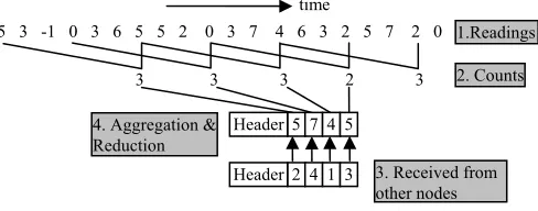
As shown in Figure 3, there are four steps of data processing at each single sensor node. First, a stream of readings are samples, next a count stream is generated according to the window size, then the node receives from other nodes their local results, and finally the node aggregates the results together and conduct data reduction by using techniques introduced in Section III.
The criteria of choosing the best query plan lies on the satisfaction of query issuer to the best extent, by taking all the factors in the weight item (i.e. power, time delay, accuracy, and error probability) in to account. Moreover, there are two obvious constraints affecting the decision making. First, size of the integrated data packet should be less than MPS. Second, the delay constraint specified with the query should be obeyed.
Therefore, the problem under study can be formalized as two questions:
Question 1: how to find the best number of samples, ns
in one window size (i.e. sample frequency, see step 1 in Figure 3), and
Question 2: how to find the maximal number of sample
data (can be 1), ni to be integrated (step 4 in Figure 3), so that trade-off denoted by the weight item leads to optimal result.
B. Proposed algorithm
The answer of Question 1 has nothing to do with data transmission, but only data processing. This means only power consumption and accuracy need to be considered, without taking delay and error rate into account. Therefore, following node cost function can be defined as
C1(ns)= A (n )
W W
W ) n ( E W W
W
s ' R a p
a s
' P a p
p ⋅
+ + ⋅
+ (8)
where Wp and Wa are the weights assigned to factors
power and accuracy respectively, and E'P(ns)and
) n ( A s
'
R are normalized energy consumption of data
processing and accuracy reciprocal respectively. The cost 5 3 -1 0 3 6 5 5 2 0 3 7 4 6 3 2 5 7 2 0
3 3 3 2 3 time
5 7 Header 4 5
1.Readings
4. Aggregation & Reduction
2. Counts
Figure 3. Data processing in a node. 2 4
function denotes the total energy and accuracy costs of one specific window size, the less the better. Normalization of power consumption and accuracy reciprocal needs more study. First, since power consumption results only from data processing, according to formula (2), the energy cost is given by
EP(ns) = ns (ES + ECUDRU), (9) where ES is sample energy, ECU is unit energy for Count
operation, and DRU is the size of one reading data. To perform the formalization, we need to find out the maximum possible number of sample in the sliding window, ns-MAX. Obviously, we can simply assume that the maximum sample rate occurs in the case the node samples each time when the node wakes up. However in practice, the real maximum sample rate must be much lower than the case. This is because the lifetime goal of a sensor network is often explicitly defined. In [12] the maximum sample rate (in samples per hour) is estimated according to the remaining battery capacity of the node, the specified lifetime of the sensor network, and the energy to collect and transmit samples. Taking advantage of this estimation, the formalization of the energy cost is given by ) n ( E ) n ( E ) n ( E MAX s P s P s ' P −
= . (10)
The accuracy of the result is represented by the reciprocal of the length of the confidence interval, and thus is relies on the estimation method. The Boolean result of whether an attribution is larger than a threshold (S.temperature > 4 C in the example) is a random variable whose probability distribution is (0 – 1), i.e. P
(ValueOfAttribute > Threshold) = p. Query is used to
estimate this probability, p by p = Count / ns. As to (0 – 1) distribution, its expectation is p and variance is p(1-p). According to Central Limit Theorem, when number of samples is big, the distribution of
) p ( p n p n Count s s − −
1 is
approximately N (0, 1). Therefore, the accuracy of the estimation with ns samples is given by
2 2 / s s z n ) n ( A α ⋅ σ
= , (11)
where σ is the variance and zα/2 is the α quantile of
standard normal distribution. The minimum accuracy can
be easily obtained by
2 2 / MIN s MIN s MIN z n ) n ( A α −
− = σ⋅ , where
ns-MIN is given by ns-MIN = rMIN Tw.
The normalized accuracy reciprocalA (ns) '
R is given by
) n ( A ) n ( A ) n ( A s MIN s s '
R = − . (12)
Note that even the variance is unknown, the normalization can still be performed.
By using formula (10) and (12) to (8), we can obtain
' s
n = arg min ns (C1(ns)). (13) Thus, the answer of Question 1 is given by
ns = (ns-MIN < ' s
n <ns-MAX, ' s n ,( '
s
n >ns-MAX: ns-MAX, ns-MIN)). (14)
The answer of Question 2 concerns both local data processing (step 2 to 4 in Figure 3) and data transmission. Suppose a data integration technique is to be utilized above a stream of results (local counts or counts received from other nodes), the algorithm focuses on finding the maximal number of samples, ni that optimizes trade-off items of the query. According to the MPS, delay, and error constraints, we have the following three arguments. For any selected node u, first,
ni1(u)= arg maxni (D’(u) < MPS), (15)
where, according to formula (1), size of data after data reduction D’(u) = D(u) (1-ru) = (Header_Size + ni DCU)(1-ru), with DCU the size of one count result (most probably attached with a sequence number of time stamp). Second,
ni2(u)= arg maxni (dW(u) < dMAX), (16)
where dW (u) = (ni– 1) Ti + T(D’(u): u->s) denotes the time of waiting and sending the integrated packet. Third,
ni3(u)= arg maxni (ep(ni) < eMAX), (17)
where ep(ni) = 1 – (1 – eb(u))D’(u) is the packet error rate
and eb is the bit error rate of the link from local node to its parent node. The eb is affected by both the data transmission rate and the signal power margin, and can be obtained from empirical estimation.
Finally, a global cost function, C2 can be defined as
C2(ni)=
) n ( e W W ) n ( d W W ) n ( E W W i ' p e d p e i ' T P e d p d i ' T P e d p
p ⋅ + ⋅ + ⋅
+ + + + + + + + (18)
where Wp+d+e= Wp+Wd+We, and E’, d’ and e’ are formalized energy consumption, time delay and packet error rate respectively. The cost function denotes the total costs of one specific query plan, the less the better. Normalization of power consumption, time delay and error rate can be performed as follows.
∑
∀
+ ⋅ + −>
> − =
u i CU
i '
T
P n E((D Header_Size):u s)
MAX
) u ( D b u
i ' p
e
)) u ( e ( ( )
n ( e
'
MAX
− −= ∀
1 1
related . (21)
Note that here the energy consumption and time delay concerns both data processing (as depicted in Figure 3) and data transmission during the entire path from local node to sink (refer to formula (6) and (7)).
After the definition of the cost function in formular (6), we have
ni4 = arg minniC2(ni) (22)
And finally, the number of samples is given by
ni = min (ni1, ni2, ni3, ni4) (23) We then solve the two questions mentioned above, and thus have the key algorithm for the query optimization.
VI. QUERY WITH DIRECT AGGREGATION
Direct aggregation is different from stepwise aggregation in the sense that, direct aggregation cannot be performed until all the aggregation data is available. In other words, it cannot be executed above partial data. In this section, without loosing any generality, we simple take MEDIAN as an example.
As to the case of query with direct aggregation, after the discussion in Section V, it will be easy to obtain. Basically, the same assumptions hold, and there are two similar questions to be solved. In this section, we focus mostly on the differences and the changes needed comparing to those in the previous section. Figure 4 illustrated the basic idea and key processes of this sort of query.
The most crucial difference the sliding window based continuous MEDIAN query (query example 1) with the one in Section V (COUNT query over stream data, query example 2) is that in query 2 COUNT is a monotonic and summary aggregate which means its value can only get larger as more values are aggregated, while on the other hand allows partial aggregation with other count values (as step 4 in Figure 3). Instead as for query 1, MEDIAN is an exemplary aggregate computing some property over the entire set of values, and therefore does not allow partial aggregation. In other words, the aggregation cannot be performed until all the concerned data is
available. This means in query 1 there will be more data transmission.
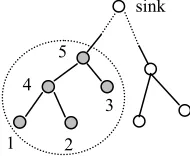
Figure 5 shows a simple example. The streams of data at node 1-4 should first be sent to node 5 (the common ancestor of all the concerned nodes except node 5 itself), and after that count a stream of median values to be sent to the sink. The relay node 4 will only forwards the readings from node 1 and 2, but cannot perform the MEDIAN aggregation operation with partial data of node 1 and 2 and local ones. Note that data reduction techniques can be used in the transmission of both original readings from node 1-4 to 5, and final average results from node 5 to the sink.
Obviously, the query is executed with two steps. First, all the readings are sent to a node who is the common ancestor of all the concerned nodes (node 5 in Figure 5) for MEDIAN aggregation. Next, a stream of median aggregation results is sent to the sink. In the second step, the problem is simple and the problem of data reduction (i.e. find out the best ni) can be directly solved with the method introduced in Section V, by simply assuming
ns=1. Therefore without losing any generality, here we assume that the common ancestor node is exactly the sink node.
As to query 2 in the previous section, the answers of the two questions (i.e. to find out ns and ni) are independent. While in query 1 the key is still to find the answers for the same questions, they are actually correlated due to the time reason and therefore should be jointly considered. Also, in answering Question 1, the main difference of query 1 with query 2 is that in query 2, we need to simply concentrate on one local node, to decide the window size for it which is actually common to all the rest concerned sensor nodes. Instead, in query 1 we have to first find out the total population of samples for all the selected sensor nodes (hereafter suppose the number is m) according to the WHILE clause (S.location = Area_C as the condition in the example above), and after that uniformly assign to each node a number of samples for one window size.
After the discussions above, a global cost function for query 1 can be defined as
) n , n ( d W ) n ( E W ) n , n (
C ' s i
T P d i '
T P p i
s = + + +
) n ( e W ) n ( A
W ' i
p e s ' R
a +
+ (18’)
1 2 3 4
5
sink
Figure 5. An sensor network query example.
5 3 2 4 3 2 4 2 4 5 3 5 4 6 3 3 4 2 4 4
3 3 4 4 time
3 3 Header 4 4
1.Readings
4. Reduction
3. Median
Figure 4. Data transmission and processing.
2. Transmission 4 2 0 1 3 6 2 1 2 4 6 2 6 6 2 7 2 3 4 3
5 3 -1 0 2 4 3 3 0 0 3 7 4 3 3 2 5 7 2 0
TABLE I
PARAMETERS VALUES USED IN PERFORMANCE ANALYSIS.
System parameters
parameter value parameter value
β 100 pJ/bit/m2 Es 10 nJ/bit
γ 2 ru PM, 0.3, 0.8
ε 90 nJ/bit Header Size 15 bytes
d 10 m DRU 2 bytes EPU 20 nJ/bit MPS 2k bytes
TPU 0 ns/bit noh 10 ETU 100 nJ/bit ns-MAX. 1 / ms TTU 0.02 ms/bit
Query parameters
parameter value parameter value dMAX 1 h Tw 10 min 1-αMIN 0.9 Ti 2 min eMAX 0.01 rMIN 100 er 10 E-5
(Wp, Wt, Wa, We ) w1: (0.7, 0.0, 0.1, 0.2)
w2: (0.1, 0.0, 0.6, 0.3) All the formula (15) to (17) and (19) to (23) in previous section are applicable here for query 1, unless the Ti for getting dW should now be replaced by sample interval
Tw/ns.
Another difference is, instead of (0, 1) distribution as in query 2, here for MEDIAN aggregation, the distribution of the concerned random variable is usually assumed as either normal distribution or uniform distribution. To normal distribution the derivation is the same as previous section (formula (11) and (12)). As to uniform distribution, by using the same approximating method of Central Limit Theorem, method in previous section is still applicable.
VII. EXPERIMENTS
In this section, we validate the effectiveness of the proposed algorithm. We assume that all the sensor nodes are homogeneous. Table 1 shows the parameters values used in the performance analysis. We assume an average
TTU(e) is available and thus we can define a number of hops (noh) to represent the distance from the end node to sink (10 in this paper). We study three data reduction scenarios. The first one is based on packet merging (PM), in which the ru can be derived by
ru =
) D Sph ( n
D n Sph D
' D
RU i
RU i
+ ⋅
⋅ + − =
− 1
1 . (24)
where Sph is header size (15 bytes in this paper). The second scenario is to employ packet compression (ru1) with ru = 0.3 (ru2), and for the third ru = 0.8 (ru3). We study the example query 2 with two weight item settings: (Wp, Wt, Wa, We) = (0.6, 0.1, 0.1, 0.2) and (0.1, 0.1, 0.5, 0.3). The target sensor network is simplified so that there is only one selected node which is of 10 hops to sink.
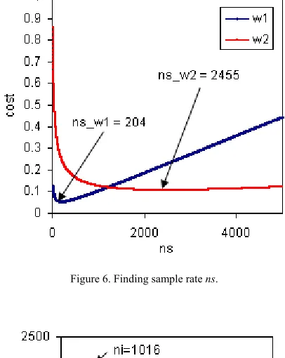
Two experiments are designed to valid the methods for answering Questing 1 and 2 respectively. Figure 6 shows the result of experiment 1. The figure clearly demonstrates the effect of the weight item. In case of w1, power consumption is deemed more important than accuracy (0.7 vs. 0.1), therefore a relatively small ns
(204) is obtained than the case of w2 (ns=2455) in which accuracy is emphasized more than energy (0.6 vs. 0.1).
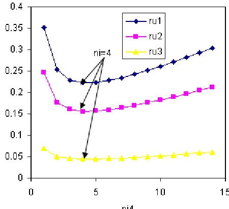
Figure 7 – 11 illustrate the results of experiment 2, in which the number of data integration ni is being found. In Figure 7, ni1 in formula (15) is found via data size.
Obviously, ru and MPS play key roles for this
calculation. In Figure 8, ni2 in formula (16) is found via waiting time. In our setting the maximum delay allowed is large, and so the time for data processing and transmission is tiny. The resulted number thus is depended mostly on sliding increment vs. delay. This is why the three scenarios of ru1-3 all return the same result. Figure 9 depicts the result of finding ni3 via packet error rate. Again D’(u) is the key factor influencing the results.
Figure 6. Finding sample rate ns.
Figure 8. Finding integration number ni2 via waiting time.
Figure 10. Finding number ni4 via cost function for w1 case.
Figure 10 and 11 are more interesting, illustrating the trade-offs between error rate and power consumption. The effect of time delay is neglected because the setting is large (1 hour) and therefore the item in the weight is set to 0 for both w1 and w2. When n is small, the cost is relatively high. Then cost decreases with increasing n. This is the benefit gaining from energy saving due to data reduction. From some point of n, the cost starts to increase again. This is because the increase in packet size leads to the increase of packet error rate. This effect is much clearer in case of w2, if comparing the two figures. This is due to the fact that w2 considers error rate more than power consumption. Finally, it is easy to understand that large ru always performs better.
VIII. CONCLUSIONS
A novel method is proposed to optimize the execution of periodical queries with COUNT and AVERAGE aggregations, by jointly considering four QoS factors including energy consumption, time delay, result accuracy and packet error rate. Algorithm is described in detail. Experiments are conducted to validate the method.
Figure 9. Finding integration number ni3 via packet error rate.
Figure 11. Finding number ni4 via cost function for w2 case.
Results show that the proposed method can achieve the goal of query optimization. Future work includes to study the effectiveness of adaptive sampling rate, smart sampling (not with fixed interval), and sample dropping schemes.
ACKNOWLEDGMENT
Financial support by Academy of Finland (Project No.: 209570) is gratefully acknowledged.
REFERENCES
[1] Johannes Gehrke and Ling Liu, “Sensor-network applications,” IEEE Internet Computing, vol. 10, no. 2, 2006, pp. 16-17.
[2] H. Gharavi and S.P. Kumar, “Special Issue on Sensor Networks and Applications,” Proceedings of the IEEE, vol. 91, no. 8, Aug. 2003.
[3] Matthew J. Miller and Nitin H. Vaidya, “A MAC Protocol to Reduce Sensor Network Energy Consumption Using a Wakeup Radio,” IEEE Transaction on Mobile Computing, Vol. 4, No. 3, 228-242, May/June 2005.
wavelength routed networks,” Proc. Workshop on High Performance Switching and Routing, 416-420, May 2005. [5] Lingxuan Hu and David Evans, “Localization for Mobile
Sensor Networks,” Proc. Tenth Annual International Conference on Mobile Computing and Networking
(MobiCom 2004). Philadelphia, 45-57, Sept.-Oct. 2004. [6] J.N. Al-Karaki and A.E. Kamal, “Routing techniques in
wireless sensor networks: a survey,” IEEE Wireless Communications, vol. 11, no. 6, 6-28, Dec. 2004.
[7] Alan Demers, Johannes Gehrke, Raimohan Rajaraman, Niki Trigoni, and Yong Yao. Energy-Efficient Data Management for Sensor Networks: A Work-In-Progress Report. 2nd IEEE Upstate New York Workshop on Sensor Networks. Syracuse, NY, October 2003.
[8] Yi Zou and Krishnendu Chakrabarty, “Energy-Aware Target Localization in Wireless Sensor Networks,” Proc. 1st IEEE International Conference on Pervasive
Computing and Communications (PerCom’03), 60-67,
Dallas-Fort Worth, Texas, USA, Mar. 2003.
[9] Ramesh Govindan, Joseph M. Hellerstein, Wei Hong, Samuel Madden, Michael Franklin, and Scott Shenker, “The sensor network as a database,” USC Technical Report No. 02-771, September 2002.
[10] Philippe Bonnet, J. E. Gehrke, and Praveen Seshadri. Towards Sensor Database Systems. In Proceedings of the Second International Conference on Mobile Data Management. Hong Kong, January 2001.
[11] Samuel R. Madden, Michael J. Franklin, Joseph M. Hellerstein, and Wei Hong, “TinyDB: An Acquisitional Query Processing System for Sensor Networks,” ACM Transactions on Database Systems, vol.30, no.1, 122-173, Mar. 2005.
[12] S. Madden, M. J. Franklin, J. M. Hellerstien, and W. Hong, “The design of an acquisitional query processor for sensor networks,” in Proceedings ACM SIGMOD, pp. 491-502, June 2003, San Diego, CA, USA.
[13] J. Gehrke and S. Madden, “Query processing in sensor networks,” IEEE Pervasive Computing, vol. 3, no. 11, pp. 46-55, 2004.
[14] Y. Yao and J. Gehrke, “Query processing for sensor networks,”, In Proceedings of the First Biennial Conference on Innovative Data Systems Research (CIDR 2003), Asilomar, California, January 2003.
[15] Hailing Ju and Li Cui, “EasiPC: A Packet Compression Mechanism for Embedded WSN,” Proceedings of the 11th IEEE International Conference on Embedded and Real-Time Computing Systems and Applications (RTCSA’05), 394-399, 2005.
[16] Naoto Kimura and Shahram Latifi, “A survey on data compression in wireless sensor networks,” Proceedings of the International Conference on Information Technology: Coding and Computing (ITCC’05), vol.2, 8-13, 2005. [17] Kenneth Barr and Krste Asanovic, “Energy aware lossless
data compression,” The First International Conference on Mobile Systems, Applications, and Services (MobiSys’03), 231-244, San Francisco, CA, May 2003.
[18] Rong Xu, Zhiyuan Li, Cheng Wang, and Peifeng Ni, “Impact of data compression on energy consumption of wireless-networked handheld devices,” Proc. 23rn International Conference on Distributed Computing Systems (ICDCS’03), 302-311, May 2003.
[19] Mo Chen and Mark L. Fowler, “Data compression trade-offs in sensor networks,” Mathematics of Data/Image Coding, Compression, and Encryption VII, with Applications. Edited by Schmalz, Mark S. Proceedings of the SPIE, Volume 5561, pp. 96-107, Oct. 2004.