Densely Connected Graph Convolutional Networks for Graph to Sequence Learning

Densely Connected Graph Convolutional Networks for

Graph-to-Sequence Learning

Zhijiang Guo1∗, Yan Zhang1∗, Zhiyang Teng1,2, Wei Lu1

1_{Singapore University of Technology and Design}

8 Somapah Road, Singapore, 487372

2_{School of Engineering, Westlake University, China}

{zhijiang guo,yan zhang,zhiyang teng}@mymail.sutd.edu.sg [email protected], [email protected]

Abstract

We focus on graph-to-sequence learning, which can be framed as transducing graph structures to sequences for text generation. To capture structural information associated with graphs, we investigate the problem of encoding graphs using graph convolutional networks (GCNs). Unlike various existing approaches where shallow architectures were used for capturing local structural information only, we introduce a dense connection strategy, proposing a novel Densely Connected Graph Convolutional Network (DCGCN). Such a deep architecture is able to integrate both local and non-local features to learn a better structural representation of a graph. Our model outperforms the state-of-the-art neural models significantly on AMR-to-text generation and syntax-based neural machine translation.

1 Introduction

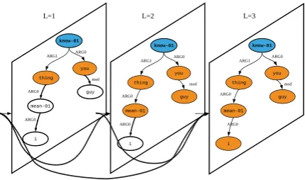
Graphs play an important role in natural language processing (NLP) as they are able to capture richer structural information than sequences and trees. Generally, semantics of sentences can be encoded as graphs. For example, the abstract meaning representation (AMR) (Banarescu et al., 2013) is a directed, labeled graph as shown in Figure 1, where nodes in the graph denote semantic concepts and edges denote relations between concepts. Such graph representations can capture rich semantic-level structural information, and are attractive representations useful for semantics-related tasks such as semantic parsing (Guo and Lu, 2018) and natural language generation (Beck et al., 2018). In this paper, we focus on the graph-to-sequence

∗_{Contributed equally.}

learning tasks, where we aim to learn repre-sentations for graphs that are useful for text generation.

Graph convolutional networks (GCNs) (Kipf and Welling, 2017) are variants of convolutional neural networks (CNNs) that operate directly on graphs, where the representation of each node is iteratively updated based on those of its adja-cent nodes in the graph through an information propagation scheme. For example, the first layer of GCNs can only capture the graph’s adjacency information between immediate neighbors, while with the second layer one will be able to cap-ture second-order proximity information (neigh-borhood information two hops away from one node) as shown in Figure 1. Formally, L layers will be needed in order to capture neighborhood information that isLhops away.

GCNs have been successfully applied to many NLP tasks (Bastings et al., 2017; Zhang et al., 2018b). Interestingly, although deeper GCNs with more layers will be able to capture richer neigh-borhood information of a graph, empirically it has been observed that the best performance is achieved with a 2-layer model (Li et al., 2018).

Therefore, recent efforts that leverage recurrence-based graph neural networks have been explored as the alternatives to encode the structural infor-mation of graphs. Examples include graph-state long short-term memory (LSTM) networks (Song et al., 2018) and gated graph neural networks (GGNNs) (Beck et al., 2018). Deep architectures based on such recurrence-based models have been successfully built for tasks such as language gener-ation, where rich neighborhood information cap-tured was shown useful.

Compared with recurrent neural networks, con-volutional architectures are highly parallelizable and are more amenable to hardware acceleration

297

Figure 1: A 3-layer densely connected graph convo-lutional network. The example AMR graph here corre-sponds to the sentence ‘‘You guys know what I mean.’’ Every layer encodes information about immediate neighbors and 3 layers are needed to capture third-order neighborhood information (nodes that are 3 hops away from the current node). Each layer concatenates all preceding outputs as the input.

(Gehring et al., 2017). It is therefore worthwhile to explore the possibility of applying deeper GCNs that are able to capture more non-local information associated with the graph for graph-to-sequence learning. Prior efforts have tried to train deep GCNs by incorporating residual con-nections (Bastings et al., 2017). Xu et al. (2018) show that vanilla residual connections proposed by He et al. (2016) are not effective for graph neural networks. They next attempt to resolve this issue by adding additional recurrent layers on top of graph convolutional layers. However, they are still confined to relatively shallow GCNs archi-tectures (at most 6 layers in their experiments), which may not be able to capture the rich non-local interactions for larger graphs.

In this paper, to better address the issue of learning deeper GCNs, we introduce dense con-nectivity to GCNs and propose the novel densely connected graph convolutional networks (DCGCNs), inspired by DenseNets (Huang et al., 2017) that distill insights from residual connections. The dense connectivity strategy is illustrated in Figure 1 schematically. Direct connections are introduced from any layer to all its preceding layers. For example, the third layer receives the outputs of the first layer and the second layer, capturing the first-order, the second-order, and the third-order neighborhood information. With the help of dense connections, we are able to train multi-layer GCN models with a large depth, allowing rich local and non-local information to be captured for learning

a better graph representation than those learned from the shallower GCN models.

Experiments show that our model is able to achieve better performance for graph-to-sequence learning tasks. For the AMR-to-text generation task, our model surpasses the current state-of-the-art neural models trained on LDC2015E86 and LDC2017T10 by 2 and 4.3 BLEU points, respectively. For the syntax-based neural machine translation task, our model is also consistently bet-ter than others, showing the effectiveness of the model on a large training set. Our code is avail-able at https://github.com/Cartus/ DCGCN.1

2 Densely Connected GCNs

In this section, we will present the basic com-ponents used for constructing our DCGCN model.

2.1 GCNs

GCNs are neural networks that operate directly on graph structures (Kipf and Welling, 2017). Here we mathematically illustrate how multi-layer GCNs work on an undirected graphG = (V,E), where V and E are the set of nodes and edges, respectively. The convolution computation for node v at the l-th layer, which takes the input feature representationh(l−1) as input and outputs the induced representation h(vl), can be defined

as

h(_vl) =ρ

u∈N(v)

W(l)h(_ul−1)+b(l)

(1)

where W(l) _{is the weight matrix, b}(l) _{is the bias} vector, N(v) is the set of one-hop neighbors of nodev, andρis an activation function (e.g., RELU [Nair and Hinton, 2010]).h(0)v is the initial input

xv, where xv ∈ Rd and d is the input feature

dimension.

GCNs with Residual Connections. Bastings et al. (2017) integrate residual connections (He et al., 2016) into GCNs to help information propagation. Specifically, each node is updated

1_{Our implementation is based on MXNET (Chen et al.,}

according to Equation (1) first and then the result-ing representation is combined with the node’s representation from the last iteration:

h(_vl) =ρ

u∈N(v)

W(l)h(_ul−1)+b(l)

+h(_vl−1) (2)

GCNs with Layer Aggregations. Xu et al. (2018) propose layer aggregations for GCNs, in which the final representation of each node is computed by combining the node’s representa-tions from all GCN layers:

hf inal_v =LA(h(_vl),h(_vl−1), . . . . ,h(1)_v ) (3)

where theLAfunction can be concatenation, max-pooling, or LSTM-attention operations as defined in Xu et al. (2018).

2.2 Dense Connectivity

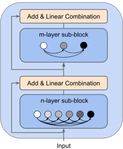
Dense connectivity is the core component of the proposed DCGCN. With dense connectivity, node v in the l-th layer not only takes inputs from h(l−1)_{, but also receives information from} all the preceding layers, as shown in Figure 2. Mathematically, we first defineg(ul)as the

concat-enation of the initial node representation and the node representations produced in layers 1, · · ·,

l−1:

g(_ul) = [xu;h(1)_u ;. . .;h(_ul−1)]. (4)

Such a mechanism allows deeper layers to capture all previous information to alleviate the problem discussed in Section 1 in graph neural networks. Similar strategies are also proposed in previous work (He et al., 2016; Huang et al., 2017).

While dense connectivity allows training deeper neural networks, every intermediate layer is designated to be of very small size, allowing adding only a small set of feature-maps at each layer. The final classifier makes predictions based on all feature-maps, which is called ‘‘collective knowledge’’ (Huang et al., 2017). Such a strategy improves the parameter efficiency. In practice, the dimensions of these small hidden layers dhidden

are decided by the number of layers L and the input feature dimension d. In DCGCN, we use

dhidden=d/L.

For example, if we have a 3-layer (L = 3) DCGCN model and input dimension is 300 (d = 300), the hidden dimension of each layer will be dhidden = d/L = 300/3 = 100. Then

Figure 2: Each DCGCN block has two sub-blocks. Both of them are densely connected graph convolutional layers with different numbers of layers. A linear trans-formation is used between two sub-blocks, followed by a residual connection.

we concatenate the output of each layer to form the new representation. We have 3 layers so the output dimension is 300 (3 × 100). Different from the GCN model whose hidden dimension is larger than or equal to the input dimension, the DCGCN model shrinks the hidden dimension as the number of layers increases in order to improve the parameter efficiency similar to DenseNets (Huang et al., 2017).

Accordingly, we modify the convolution com-putation of each layer as:

h(_vl) =ρ

u∈N(v)

W(l)g(_ul)+b(l)

(5)

The column dimension of the weight matrix increases by dhidden per layer, that is, W(l) ∈ Rdhidden×d(l)_{, whered}(l) _=d+d

hidden×(l−1).

2.3 Graph Attention

In order to perform self-attention on nodes, attention coefficients are required. The input for the calculation is a set of vectors, ˜g(l) ₌

{g˜(₁l),˜g₂(l), . . . ,˜gn(l)}, after node-wise feature

trans-formation ˜g(ul) = W(l)g

(l)

u . As an initial step,

a shared linear projection parameterized by a weight matrix,Wa ∈Rdhidden×dhidden, is applied

to nodes in the graph. Attention coefficients can be computed as:

α(_ijl) = exp

φa[Wa˜g

(l)

i ;Wa˜g

(l)

j ]

k∈Niexp

φa[Wa˜g

(l)

i ;Wa˜g

(l)

k ]

(6)

where a ∈ R2dhidden _{is a weight vector, φ is}

the activation function (here we use LeakyReLU [Girshick et al., 2014]). These coefficients are used to compute a linear combination of the node representations. Modifying the convolution computation for attention, we arrive at:

h(_vl)=ρ

u∈N(v)

α(_vul)W(l)g(_ul)+b(l)

(7)

where α(vul) are normalized attention coefficients

computed by the attention mechanism atl-th layer. Note that these coefficients will not change the dimension of the output representations.

3 Graph-to-Sequence Model

In the following we will explain the model ar-chitecture of the graph-to-sequence model. We leverage DCGCNs as the graph encoder, which directly models the graph structure without linearization.

3.1 Graph Encoder

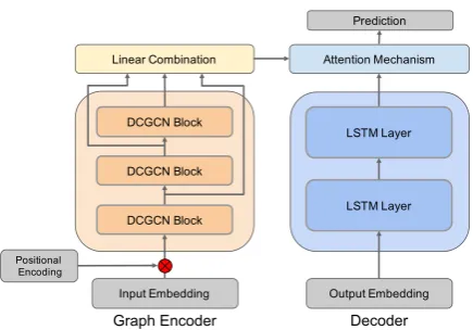
The graph encoder is composed of DCGCN blocks, as shown in Figure 3. Within each DCGCN block, we design two types of multi-layer DCGCNs as two sub-blocks to capture graph structure at different abstract levels. As Figure 2 shows, in each block, the first sub-block has n-layers and the second sub-block hasm-layers. This prototype shares the same spirit with the usage of two different-sized filters in DenseNets (Huang et al., 2017).

Linear Combination Layer. In addition to densely connected layers, we include a linear

Figure 3: The model concatenates node embeddings and positional embeddings as inputs. The encoder con-tains a stack ofN identical blocks. The linear trans-formation layer combines output of all blocks into hidden representations. These are fed into an attention mechanism, generating the context vector. The decoder, a 2-layer LSTM (Hochreiter and Schmidhuber, 1997), makes predictions based on hidden representations and the context vector.

combination layer between multi-layer DCGCNs to filter the representations from different DCGCN layers, reaching a more expressive representation. This strategy is inspired by ELMo (Peters et al., 2018), which combines the hidden states from different LSTM layers. We also use a residual connection (He et al., 2016) to incorporate the initial inputs of multi-layer GCNs into the linear combination layer, see Figure 3. Formally, the output of the linear combination layer is defined as:

hcomb =Wcomb

hout+xv

+bcomb (8)

wherehoutis the output of the densely connected

layers by concatenating outputs from all previous

L layers hout = [h(1);. . .;h(L)]and hout ∈ Rd.

xv is the input of the DCGCN layer.hout andxv

share the same dimensiond. Wcomb ∈ Rd×d is a

weight matrix and bcomb is a bias vector for the

linear transformation. BothWcombandbcomb are

different according to different DCGCN layers. In addition, another linear combination layer is added to obtain the final representations as shown in Figure 3.

3.2 Extended Levi Graph

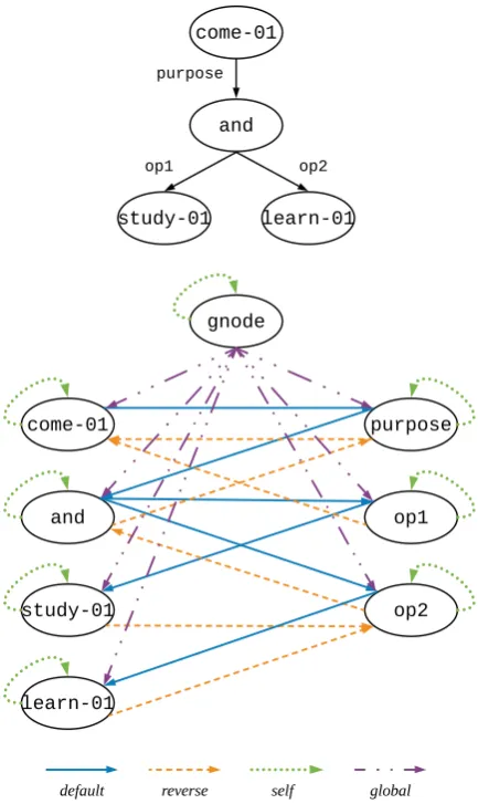
transformations. Marcheggiani and Titov (2017) add reverse edges as well as self-loop edges for each node to the original graph. This strategy is similar to the bidirectional recurrent neural networks (RNNs) (Elman, 1990), which can enjoy the information propagation from two directions. Beck et al. (2018) adapt this approach and addi-tionally transform the directed input graphs into Levi graphs (Gross et al., 2013). Basically, edges in the original graphs are turned into additional nodes in Levi graphs. With this approach, we can encode the original edge labels and node inputs in the same way. Specifically, Beck et al. (2018) define three types of edge labels on the Levi graph: default, reverse, and self, which refer to the original edges, the new virtual edges that are reverse to the original edges, and the self-loop edges.

Scarselli et al. (2009) add another node that is connected to all other nodes. Zhang et al. (2018a) use a global sentence-level node to assemble and back-distribute information. Motivated by these works, we propose anextended Levi graph, which adds a global node in the Levi graph. For every node x in the original Levi graph, there is a new edge (global) from the global node to x. Figure 4 shows an example AMR graph and its corresponding extended Levi graph. The edge type vocabulary for the extended Levi graph of the AMR graph now becomesT ={default,reverse,

self,global}. Our motivations are three-fold. First, the global node gives each node a global view of the input graph, which can make each node more aware of the non-local information. Second, the global node can serve as a hub to help node communications, which can facilitate the node information propagation process. Third, the output vectors of the global node in the encoder can be used as the initial states of the decoder, which are crucial for sequence-to-sequence learning tasks. Prior efforts average representations of all nodes as the graph embedding to initialize the decoder. Instead, we directly use the learned representation of the global nodes, which captures the infor-mation from all nodes in the whole graph.

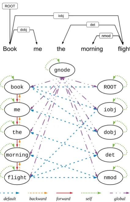
The input to the syntax-based neural machine translation task is the dependency tree. Unlike the AMR graph, the sentence contains significant sequential information. Beck et al. (2018) inject this information by adding sequential connections to each token. In our model, we also add for-ward and backfor-ward sequential connections, as

Figure 4: An AMR graph (top) and its corresponding extended Levi graph (bottom). The extended Levi graph contains an additional global node and four different type of edges.

illustrated in Figure 5. Therefore, the edge type vocabulary for the extended Levi graph of the dependency tree becomesT ={default,reverse,

self,global,forward,backward}.

Positional encodings about the relative or absolute position of the tokens have been proved beneficial for sequence learning (Gehring et al., 2017). We also include positional encodings by concatenating them with the learned word embeddings. The positional encodings are indexed by integer values representing the minimum dis-tance from the root node. For example, come-01

Figure 5: A dependency tree and its extended Levi graph.

3.3 Direction Aggregation

Directionality and edge labels play an important role in linguistic structures. Information from in-coming edges, outgoing edges, and self edges should be treated differently by using separate weight matrices. Moreover, information from incoming edges that have different labels should have different weight matrices, too. Following this motivation, we incorporate the directionality of an edge directly in its label. For example, node learn-01 in Figure 4 has three incoming edges, these edges have three different types: default (from nodeop2),self (from nodelearn-01), andglobal

(from nodegnode). For the AMR graph we have four types of edges while for dependency trees we have six as mentioned in Section 3.2. Thus, considering different type of edges, we modify the convolution computation as:

v(_tl) =ρ

u∈N(v)

dir(u,v)=t

α(_vul)W_t(l)g(_ul)+b(_tl)

(9)

wheredir(u, v)selects the weight matrix and bias term associated with the edge typet. For example, in the AMR generation task, there are four edge types:default,reverse,self,andglobal. Each type corresponds to a separate weight matrix and a separate bias term.

Now we need to aggregate representations learned from different types of edges. A simple way to do this is averaging them to get the fi-nal representations. However, Hamilton et al. (2017) show that using a mean-based function to aggregate feature information from different nodes may not be satisfactory, since informa-tion from different sources should not be treated equally. Thus we assign different weights to infor-mation from different types of edges to integrate such information. Specifically, we concatenate the learned representations from all types of edges and perform a linear transformation, mathemati-cally represented as:

f([v₁(l);· · ·;v(_Tl)]) =Wf[v

(l) 1 ;· · · ;v

(l)

T ] +bf

(10) whereWf ∈Rd

_×d

hidden _{is the weight matrix and}

d = T ×dhidden. T is the size of the edge type

vocabulary and dhidden is the hidden dimension

in DCGCN layers as described in Section 2.2. bf ∈ Rdhidden is a bias vector. Finally, the

con-volution computation becomes:

h(_vl) =ρ

f([v(₁l);· · · ;v(_Tl)])

(11)

3.4 Decoder

We use an attention-based LSTM decoder (Bahdanau et al., 2015). The initial state of the decoder is the representation of the global node described in Section 3.2. The decoder yields the natural language sequence by calculating a sequence of hidden states sequentially. Here we also include the coverage mechanism (Tu et al., 2016). Therefore, when generating thet-th token, the decoder considers five factors: the attention memory, the word embedding of the (t−1)-th token, the previous hidden state of LSTM, the previous context vector, and the previous coverage vector.

4 Experiments

4.1 Experimental Setup

Dataset Train Dev Test

AMR15 (LDC2015E86) 16,833 1,368 1,371 AMR17 (LDC2017T10) 36,521 1,368 1,371

English-Czech 181,112 2,656 2,999 English-German 226,822 2,169 2,999

Table 1: The number of sentences in four datasets.

including AMR-to-text generation and syntax-based neural machine translation (NMT). For the AMR-to-text generation task, we use two benchmarks—the LDC2015E86 dataset (AMR15) and the LDC2017T10 dataset (AMR17). In these datasets, each instance contains a sentence and an AMR graph. We follow Konstas et al. (2017) to apply entity simplification in the preprocessing steps. We then transform each preprocessed AMR graph into its extended Levi graph as described in Section 3.2. For the syntax-based NMT task, we evaluate our model on both the En-De and the En-Cs News Commentary v11 dataset

from the WMT16 translation task.2 We parse

English sentences after tokenization to generate the dependency trees on the source side using SyntaxNet (Alberti et al., 2017).3 We tokenize Czech and German using the Moses tokenizer.4 On the target side, we use byte-pair encodings (Sennrich et al., 2016) with 8,000 merge oper-ations to obtain subwords. We transform the labelled dependency trees into their corresponding extended Levi graphs as described in Section 3.2. Table 1 shows the statistics of these four datasets. The AMR-to-text datasets contain about 16 K

∼ 36 K training instances. The NMT datasets

are relatively large, consisting of around 200 K training instances.

We tune model hyper-parameters using random layouts based on the results of the development set. We choose the number of DCGCN blocks (Block) from {1,2,3,4}. We select the feature dimensiondfrom {180,240,300,360,420}. We do not use pretrained embeddings. The encoder and the decoder share the training vocabulary. We adopt Adam (Kingma and Ba, 2015) with an initial learning rate of 0.0003 as the optimizer. The

2 http://www.statmt.org/wmt16/translation-task.html.

3_{https://github.com/tensorflow/models/tree/} master/research/syntaxnet.

4_{https://github.com/moses-smt/mosesdecoder.}

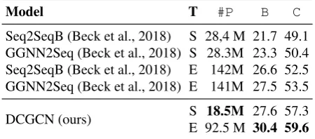
Model T #P B C

Seq2SeqB (Beck et al., 2018) S 28,4 M 21.7 49.1 GGNN2Seq (Beck et al., 2018) S 28.3M 23.3 50.4 Seq2SeqB (Beck et al., 2018) E 142M 26.6 52.5 GGNN2Seq (Beck et al., 2018) E 141M 27.5 53.5

DCGCN (ours) S 18.5M 27.6 57.3 E 92.5 M 30.4 59.6

Table 2: Main results on AMR17. #P shows the

model size in terms of parameters; ‘‘S’’ and ‘‘E’’ denote single and ensemble models, respectively.

batch size (Batch) candidates are {16,20,24}. We determine when to stop training based on the perplexity change in the development set. For decoding, we use beam search with beam size 10. Through preliminary experiments, we find that the combinations (Block= 4,d= 360,Batch= 16) and (Block= 2,d= 360,Batch= 24) give best results on AMR and NMT tasks, respectively. Following previous work, we evaluate the results in terms of both BLEU (B) scores (Papineni et al., 2002) and sentence-level CHRF++ (C) scores (Popovic, 2017; Beck et al., 2018). Particularly, we use case-insensitive BLEU scores for AMR and case sensitive BLEU scores for NMT. For ensemble models, we train five models with different random seeds and then use Sockeye (Felix et al., 2017) to perform default ensemble decoding.

4.2 Main Results on AMR-to-text Generation

We compare the performance of DCGCNs with the other three kinds of models: (1) sequence-to-sequence (Seq2Seq) models, which use linearized graphs as inputs; (2) recurrent graph encoders (GGNN2Seq, GraphLSTM); (3) models trained with external resources. For convenience, we denote the LSTM-based Seq2Seq models of Konstas et al. (2017) and Beck et al. (2018) as Seq2SeqK and Seq2SeqB, respectively. GGNN2Seq (Beck et al., 2018) is the model that leverages GGNNs as graph encoders.

5.9 more BLEU points than the single models of Seq2SeqB on AMR17. These results demonstrate the importance of explicitly capturing the graph structure in the encoder.

In addition, our single DCGCN model obtains better results than previous ensemble models. For example, on AMR17, the single DCGCN model is 1 BLEU point higher than the ensemble model of Seq2SeqB. Our model requires substantially fewer parameters (e.g., the parameter size is only 3/5 and 1/9 of those in GGNN2Seq and Seq2SeqB, respectively). The ensemble approach based on combining five DCGCN models initialized with different random seeds achieves a BLEU score of 30.4 and a CHRF++ score of 59.6.

Under the same setting, our model also consis-tently outperforms graph encoders based on recurrent neural networks or gating mechanisms. For GGNN2Seq, our single model is 3.3 and 0.1 BLEU points higher than their single and ensemble models, respectively. We also have similar observations in terms of CHRF++ scores for sentence-level evaluations. DCGCN also out-performs GraphLSTM by 2.0 BLEU points in the fully supervised setting as shown in Table 3. Note that GraphLSTM uses char-level neural representations and pretrained word embeddings, whereas our model solely relies on word-level representations with random initializations. This empirically shows that compared with recurrent graph encoders, DCGCNs can learn better rep-resentations for graphs.

Moreover, we compare our results with the state-of-the-art semi-supervised models on the AMR15 test set (Table 3), including non-neural methods such as TSP (Song et al., 2016), PBMT (Pourdamghani et al., 2016), Tree2Str (Flanigan et al., 2016), and SNRG (Song et al., 2017). All these non-neural models train language models on the whole Gigaword corpus. Our ensemble model gives 28.2 BLEU points without external data, which is better than these other methods.

Following Konstas et al. (2017) and Song et al. (2018), we also evaluate our model using external Gigaword sentences as training data. We first use the additional data to pretrain the model, then fine tune it on the gold data. Using additional 0.1M data, the single DCGCN model achieves a BLEU score of 29.0, which is higher than Seq2SeqK (Konstas et al., 2017) and GraphLSTM (Song et al., 2018) trained with 0.2M additional data. When using the same amount of 0.2M data, the

Model External B

Seq2SeqK (Konstas et al., 2017) − 22.0 GraphLSTM (Song et al., 2018) − 23.3

DCGCN(single) − 25.7

DCGCN(ensemble) − 28.2

TSP (Song et al., 2016) ALL 22.4 PBMT (Pourdamghani et al., 2016) ALL 26.9 Tree2Str (Flanigan et al., 2016) ALL 23.0 SNRG (Song et al., 2017) ALL 25.6

Seq2SeqK (Konstas et al., 2017) 0.2M 27.4 GraphLSTM (Song et al., 2018) 0.2M 28.2

DCGCN(single) 0.1M 29.0 DCGCN(single) 0.2M 31.6

Seq2SeqK (Konstas et al., 2017) 2M 32.3 GraphLSTM (Song et al., 2018) 2M 33.6 Seq2SeqK (Konstas et al., 2017) 20M 33.8

DCGCN(single) 0.3M 33.2 DCGCN(ensemble) 0.3M 35.3

Table 3: Main results on AMR15 with/without external Gigaword sentences as auto-parsed data are used.

performance of DCGCN is 4.2 and 3.4 BLEU points higher than Seq2SeqK and GraphLSTM, respectively. The DCGCN model is able to achieve competitive BLEU points (33.2) by using 0.3M external data, while GraphLSTM achieves a score of 33.6 by using 2M data and Seq2SeqK achieves a score of 33.8 by using 20M data. These results show that our model is more effective in terms of using automatically generated AMR graphs. Using 0.3M additional data, our ensemble model achieves the new state-of-the-art result of 35.3 BLEU points.

4.3 Main Results on Syntax-based NMT

English-German English-Czech

Model Type #P B C #P B C

BoW+GCN (Bastings et al., 2017) Single − 12.2 − − 7.5 − CNN+GCN (Bastings et al., 2017) Single − 13.7 − − 8.7 − BiRNN+GCN (Bastings et al., 2017) Single − 16.1 − − 9.6 −

PB-SMT (Beck et al., 2018) Single − 12.8 43.2 − 8.6 36.4 Seq2SeqB (Beck et al., 2018) Single 41.4M 15.5 40.8 39.1M 8.9 33.8 GGNN2Seq (Beck et al., 2018) Single 41.2M 16.7 42.4 38.8M 9.8 33.3

DCGCN (ours) Single 29.7M 19.0 44.1 28.3M 12.1 37.1

Seq2SeqB (Beck et al., 2018) Ensemble 207M 19.0 44.1 195M 11.3 36.4 GGNN2Seq (Beck et al., 2018) Ensemble 206M 19.6 45.1 194M 11.7 35.9

DCGCN (ours) Ensemble 149M 20.5 45.8 142M 13.1 37.8

Table 4: Main results on English-German and English-Czech datasets.

with the best GCN-based model (BiRNN+GCN), our single DCGCN model surpasses it by 2.7 and 2.5 BLEU points on the En-De and En-Cs tasks, respectively. Our models consist of full GCN layers, removing the burden of using a recurrent encoder to extract non-local contextual information in the bottom layers. Compared with non-GCN models, our single DCGCN model is 2.2 and 1.9 BLEU points higher than the current state-of-the-art single model (GGNN2Seq) on the En-De and En-Cs translation tasks, respectively. In addition, our single model is comparable to the ensemble results of Seq2SeqB and GGNN2Seq, whereas the number of parameters of our models is only about 1/6 of theirs. Additionally, the ensem-ble DCGCN models achieve 20.5 and 13.1 BLEU points on the En-De and En-Cs tasks, respectively. Our ensemble results are significantly higher than those of the state-of-the-art syntax-based ensem-ble models reported by GGNN2Seq (En-De: 20.5 vs. 19.6; En-Cs: 13.1 vs. 11.7 in terms of BLEU).

4.4 Additional Experiments

Layers in the Sub-block. Table 5 shows the effect of the number of layers of each sub-block on the AMR15 development set. DenseNets (Huang et al., 2017) use two kinds of convolution filters: 1×1 and 3×3. Similar to DenseNets,

we choose the values of n and m for layers

from [1,2,3,6]. We choose this value range by considering the scale of non-local nodes, the abstract information at different level, and the calculation efficiency. For brevity, we only show representative configurations. We first inves-tigate DCGCN with one block. In general, the

Block n m B C

1

1 1 17.6 48.3

1 2 19.2 50.3

2 1 18.4 49.1

1 3 19.6 49.4

3 1 20.0 50.5

3 3 21.4 51.0

3 6 21.8 51.7

6 3 21.7 51.5

6 6 22.0 52.1

2

3 6 23.5 53.3

6 3 23.3 53.4

6 6 22.0 52.1

Table 5: The effect of the number of layers inside DCGCN sub-blocks on the AMR15 develop-ment set.

performance increases when we gradually enlarge

nandm. For example, whenn= 1andm = 1, the BLEU score is 17.6; whenn= 6andm= 6, the BLEU score becomes 22.0. We observe that the three settings (n = 6, m = 3), (n = 3,

m= 6), and (n= 6,m = 6) give similar results for both 1 DCGCN block and 2 DCGCN blocks. Because the first two settings contain fewer parameters than the third setting, it is reasonable to choose either (n= 6,m= 3) or (n= 3,m= 6). For later experiments, we use (n= 6,m= 3).

GCN B C GCN B C +RC (2) 16.8 48.1 +RC+LA (2) 18.3 47.9 +RC (4) 18.4 49.6 +RC+LA (4) 18.0 51.1 +RC (6) 19.9 49.7 +RC+LA (6) 21.3 50.8 +RC (9) 21.1 50.5 +RC+LA (9) 22.0 52.6 +RC (10) 20.7 50.7 +RC+LA (10) 21.2 52.9

DCGCN1 (9) 22.9 53.0 DCGCN3 (27) 24.8 54.7 DCGCN2 (18) 24.2 54.4 DCGCN4 (36)25.5 55.4

Table 6: Comparisons with baselines. +RC denotes GCNs with residual connections. +RC+LA refers to GCNs with both residual connections and layer

aggregations. DCGCNi represents our model

with i blocks, containing i×(n+m) layers. The number of layers for each model is shown in parentheses.

the number of GCN layers from 2 to 9 boosts the model performance. However, when the layer number exceeds 10, the performance of both baseline models start to drop. For example, GCN+RC+LA (10) achieves a BLEU score of 21.2, which is worse than GCN+RC+LA (9). In preliminary experiments, we cannot manage to train very deep GCN+RC and GCN+RC+LA models. In contrast, our DCGCN models can be trained using a large number of layers. For example, DCGCN4 contains 36 layers. When we increase the DCGCN blocks from 1 to 4, the model performance continues increasing on the AMR15 development set. We therefore choose DCGCN4 for the AMR experiments. Using a similar method, DCGCN2 is selected for the NMT tasks. When the layer numbers are 9, DCGCN1 is better than GCN+RC in term of B/C scores (21.7/51.5 vs. 21.1/50.5). GCN+RC+LA (9) is sightly better than DCGCN1. However, when we set the number to 18, GCN+RC+LA achieves a BLEU score of 19.4, which is significantly worse than the BLEU score obtained by DCGCN2 (23.3). We also try GCN+RC+LA (27), but it does not converge. In conclusion, these results show the robustness and effectiveness of our DCGCN models.

Performance vs. Parameter Budget. We also evaluate the performance of DCGCN model against different number of parameters on the AMR gen-eration task. Results are shown in Figure 6. Specif-ically, we try four parameter budgets, including 11.8M, 14.0M, 16.2M, and 18.4M. These num-bers correspond to the model size (in terms of number of parameters) of DCGCN1, DCGCN2,

DCGCN3, and DCGCN4, respectively. For each budget, we vary both the depth of GCN models and the hidden vector dimensions of each node in GCNs in order to exhaust the entire budget. For example, GCN(2)−512, GCN(3)−426,

GCN(4)−372, andGCN(5)−336contain about 11.8M parameters, whereGCN(i)−dindicates a GCN model withilayers and the hidden size for each node isd. We compare DCGCN1 with these four models. DCGCN1 gives 22.9 BLEU points. For the GCN models, the best result is obtained byGCN(5)−336, which falls behind DCGCN1 by 2.0 BLEU points. We compare DCGCN2, DCGCN3, and DCGCN4 with their equal-sized GCN models in a similar way. The results show that DCGCN consistently outperforms GCN under the same parameter budget. When the parameter budget becomes larger, we can observe that the performance difference becomes more prominent. In particular, the BLEU margins between DCGCN models and their best GCN models are 2.0, 2.7, 2.7, and 3.4, respectively.

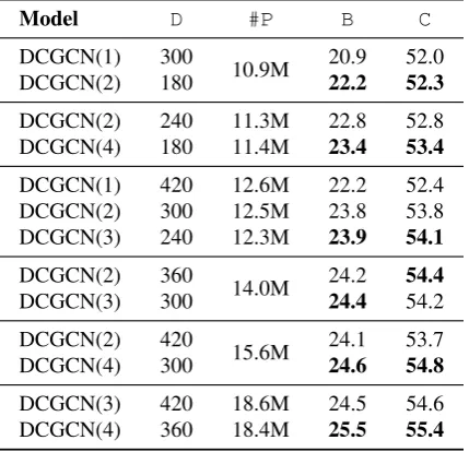
Performance vs. Layers. We compare DCGCN models with different layers under the same param-eter budget. Table 7 shows the results. For exam-ple, when both DCGCN1 and DCGCN2 are limited to 10.9M parameters, DCGCN2 obtains 22.2 BLEU points, which is higher than DCGCN1 (20.9). Similarly, when DCGCN3 and DCGCN4 contain 18.6M and 18.4M parameters, DCGCN4 outperforms DCGCN3 by 1 BLEU point with a slightly smaller model. In general, we found when the parameter budget is the same, deeper DCGCN models can obtain better results than the shallower ones.

Figure 6: Comparison of DCGCN and GCN over different number of parameters.a-b means the model hasa layers (ablocks for DCGCN) and the hidden size isb(e.g., 5-336 means a 5-layer GCN with the hidden size 336).

Model D #P B C

DCGCN(1) 300

10.9M 20.9 52.0 DCGCN(2) 180 22.2 52.3

DCGCN(2) 240 11.3M 22.8 52.8 DCGCN(4) 180 11.4M 23.4 53.4

DCGCN(1) 420 12.6M 22.2 52.4 DCGCN(2) 300 12.5M 23.8 53.8 DCGCN(3) 240 12.3M 23.9 54.1

DCGCN(2) 360

14.0M 24.2 54.4 DCGCN(3) 300 24.4 54.2

DCGCN(2) 420

15.6M 24.1 53.7 DCGCN(4) 300 24.6 54.8

DCGCN(3) 420 18.6M 24.5 54.6 DCGCN(4) 360 18.4M 25.5 55.4

Table 7: Comparisons of different DCGCN models under almost the same parameter budget.

models have the same number of layers, dense connections allow the model to achieve much better performance. If all the dense connections are not considered, the model does not coverage at all. These results indicate dense connections do play a significant role in our model.

Ablation Study for Encoder and Decoder. Following Song et al. (2018), we conduct a further ablation study for modules used in the graph encoder and LSTM decoder on the AMR15 dev set, including linear combination, global node, direction aggregation, graph attention mecha-nism, and coverage mechanism using the 4-block models by always keeping the dense connections. Table 9 shows the results. For the encoder, we find that the linear combination and the global node have more contributions in terms of B/C

Model B C

DCGCN4 25.5 55.4

-{4}dense block 24.8 54.9 -{3, 4}dense blocks 23.8 54.1 -{2, 3, 4}dense blocks 23.2 53.1

Table 8: Ablation study for density of

connections on the dev set of AMR15. -{i}dense block denotes removing the dense connections in thei-th block.

Model B C

DCGCN4 25.5 55.4

Encoder Modules

-Linear Combination 23.7 53.2

-Global Node 24.2 54.6

-Direction Aggregation 24.6 54.6 -Graph Attention 24.9 54.7 -Global Node&Linear Combination 22.9 52.4

Decoder Modules

-Coverage Mechanism 23.8 53.0

Table 9: Ablation study for modules used in the graph encoder and the LSTM decoder.

Figure 7: CHRF++ scores with respect to the input graph size for three models.

producing more expressive graph representations. Results also show the linear combination is more effective than the global node. Considering them together further enhances the model performance. After removing the graph attention module, our model gives 24.9 BLEU points. Similarly, exclud-ing the direction aggregation module leads to a performance drop to 24.6 BLEU points. The cover-age mechanism is also effective in our models. Without the coverage mechanism, the result drops by 1.7/2.4 points forB/Cscores.

4.5 Analysis and Discussion

Graph Size. Following Bastings et al. (2017), we show in Figure 7 the CHRF++ score variations according to the graph size|G|on the AMR2015 development set, where |G|refers to the number of nodes in the extended Levi graph. We bin the graph size into five classes (≤ 30,(30,40],

(40,50],(50,60], > 60). We average the sentence-level CHRF++ scores of the sentences in the same bin to plot Figure 7. For small graphs (i.e.,

|G| ≤ 30), DCGCN obtains similar results as the baselines. For large graphs, DCGCN signif-icantly outperforms the two baselines. In general, as the graph size increases, the gap between DCGCN and the two baselines becomes larger. In addition, we can also notice that the margin between GCN and GCN+LA is quite stable, while the margin between DCGCN and GCN+LA varies according to the graph size. The trend for BLEU scores is similar to CHRF++ scores. This suggests that DCGCN can perform better for larger graphs as its deeper architecture can capture the long-distance dependencies. Dense connections facil-itate information propagation in large graphs, while

(s / state-01

00:ARG0 (p / person

0000:ARG0-of (h / have-org-role-91 000000:ARG1 (i / intelligence

00000000:mod (c / country :wiki "united states" 0000000000:name (n / name :op1 "u.s."))) 000000:ARG2 (o / official)))

00:ARG1 (c2 / continue-01

0000:ARG0 (p2 / person

000000:ARG0-of (h2 / have-org-role-91 00000000:ARG2 (o2 / official

0000000000:mod (c3 / country :wiki "north korea" 000000000000:name (n2 / name :op1 "north" :op2 000000000000"korea")))))

0000:ARG1 (t / trade-01 000000:ARG1 (t2 /technology 00000000:purpose (w / weapon 0000000000:ARG2-of (d / destroy-01 000000000000:degree (m / mass)))) 000000:mod (g / globe)) 0000:ARG2-of (i2 / include-01 000000:ARG1 (i3 /instruct-01 00000000:ARG3 (m2 / make-01 00000000000:ARG1 (m3 / missile

0000000000000:ARG1-of (a / advanced-02)))))))

Reference: u.s. intelligence officials stated that north korean officials are continuing global trade intechnologyfor weapons of mass destruction includinginstructionsfor making advanced missiles.

GCN+RC: a u.s. intelligence official stated that north korea officials continued the global trade for weapons of mass destruction by making advanced missiles to make advanced missiles.

GCN+RC+LA: a u.s. intelligence official stated that north korea officials continued global trade with weapons of mass destruction including making advanced missiles.

DCGCN: a u.s. intelligence official stated that north korea officials continue global trade ontechnologyfor weapons of mass destruction includinginstructionsto make advanced missiles.

Table 10: Example outputs.

shallow GCNs might struggle to capture such dependencies.

the token level. However, the conveyed semantic information in the generated sentence largely dif-fers from that of the reference. DCGCNs do not have this problem.

5 Related Work

Our work builds on a rich line of recent efforts on graph-to-sequence models, graph convolutional networks, and densely connected convolutional networks.

Graph-to-Sequence Learning. Early research efforts for graph-to-sequence learning are based on statistical methods. Lu et al. (2009) present a language generation model using the tree-structured meaning representation based on tree conditional random fields. Lu and Ng (2011) propose a model for language generation from lambda calculus expressions that can be represented as forest structures. Konstas and Lapata (2012, 2013) lever-age hypergraphs for concept-to-text generation. Flanigan et al. (2016) transform a given AMR graph into a spanning tree, before translating it into a sentence using a tree-to-string transducer. Pourdamghani et al. (2016) adopt a phrase-based model for machine translation (Koehn et al., 2003) based on a linearized AMR graph. Song et al. (2017) leverage a synchronous node replacement grammar. Konstas et al. (2017) also linearize the input graph and feed it to the Seq2Seq model (Sutskever et al., 2014).

Sequence-based neural networks may lose struc-tural information from the original graph because they require linearization of the input graph. Recent research efforts consider developing encoders with graph neural networks. Beck et al. (2018) use GGNNs (Li et al., 2016) as the encoder and introduce the Levi graph that allows nodes and edges to have their own hidden representations. Song et al. (2018) propose the graph-state LSTM to directly encode graph-level semantics. In order to capture non-local information, the encoder performs graph state transition by information exchange between connected nodes. Their work belongs to the family of RNNs. Our graph en-coder is built based on GCNs. Recurrent graph neural networks (Li et al., 2016; Song et al., 2018) use gated operations to update node states whereas graph convolutional networks use linear transformation. The contrast between our model and theirs is reminiscent of the contrast between CNN and RNN.

Closest to our work, Bastings et al. (2017) stack GCNs upon a RNN or CNN encoder because 2-layer GCNs may not be able to capture non-local information, especially when the graph is large. Our graph encoder solely relies on the DCGCN model, whose deep network structure encodes richer local and non-local information for learning better graph representations.

Densely Connected Convolutional Networks. Intuitively, neural networks should be able to learn rich representations by stacking a large number of layers. However, empirical results often do not support such an intuition—useful information captured in earlier layers may get lost after passing through subsequent layers. Many recent efforts focus on resolving such an issue. Highway Networks (Srivastava et al., 2015) use bypassing paths along with gating units to train networks. ResNets (He et al., 2016), in which identity map-pings are used as bypassing paths, have achieved impressive performance on various tasks. DenseNets (Huang et al., 2017) refine this insight and propose a dense connectivity strategy, which connects all layers directly with each other to ensure maximum information flow between layers.

Graph Convolutional Networks. Early efforts that attempt to extend neural networks to deal with arbitrary structured graphs are introduced by Gori et al. (2005) and Scarselli et al. (2009), where the states of nodes are updated based on the states of their neighbors. Bruna (2014) then applies the convolution operation on graph Laplacians to construct efficient architectures in the spectral domain. Subsequent efforts improve its computational efficiency with local spectral convolution techniques (Henaff et al., 2015; Defferrard et al., 2016; Kipf and Welling, 2017).

Our approach is closely related to GCNs (Kipf and Welling, 2017), which restrict the filters to operate on a first-order neighborhood around each node. Recent improvements and extensions of GCNs include using additional aggregation methods such as vertex attention (Velickovic et al., 2018) or pooling mechanism (Hamilton et al., 2017) to better summarize neighborhood states.

over-smoothed output representations that impede distinguishing nodes from different clusters. Re-cent attempts that try to address this issue includes the use of layer-aggregation functions (Xu et al., 2018), which combine learned features from all layers, and the use of co-training and self-training mechanisms that encourage exploration on the entire graph (Li et al., 2018).

6 Conclusion

We introduce the novel densely connected graph convolutional networks to learn structural graph representations. Experimental results show that DCGCNs can outperform state-of-the-art models in two tasks: AMR-to-text generation and syntax-based neural machine translation. Unlike previous designs of GCNs, DCGCNs scale naturally to significantly more layers without suffering from performance degradation and optimization diffi-culties, thanks to the introduced dense connec-tivity mechanism. Such a deep architecture allows the encoder to better capture the rich structural information of a graph, especially when it is large. There are multiple venues for future work. One natural question we would like to ask is how to make use of the proposed framework to perform improved graph representation learning for various graph related tasks (Xu et al., 2018). On the other hand, we would also like to investigate how other NLP applications such as relation extraction (Zhang et al., 2018b) and semantic role labeling (Marcheggiani and Titov, 2017) can potentially benefit from our proposed approach.

Acknowledgments

We would like to thank the anonymous reviewers and our Action Editor Stefan Riezler for their comments and suggestions on this work. We would also like to thank Daniel Beck, Linfeng Song, Joost Bastings, Zuozhu Liu, and Yiluan Guo for their helpful suggestions. This work is supported by Singapore Ministry of Education Academic Research Fund (AcRF) Tier 2 Project MOE2017-T2-1-156. This work is also partially supported by SUTD project PIE-SGP-AI-2018-01.

References

Chris Alberti, Daniel Andor, Ivan Bogatyy, Michael Collins, Daniel Gillick, Lingpeng Kong,

Terry Koo, Ji Ma, Mark Omernick, Slav Petrov, Chayut Thanapirom, Zora Tung, and David Weiss. 2017. Syntaxnet models for the conll 2017 shared task. arXiv preprint arxiv:1703.04929.

Dzmitry Bahdanau, Kyunghyun Cho, and Yoshua Bengio. 2015. Neural machine translation by jointly learning to align and translate. In

Proceedings of ICLR.

Laura Banarescu, Claire Bonial, Shu Cai, Madalina Georgescu, Kira Griffitt, Ulf Hermjakob, Kevin Knight, Philipp Koehn, Martha Palmer, and Nathan Schneider. 2013. Abstract meaning representation for sembanking. InProceedings of LAW@ACL.

Joost Bastings, Ivan Titov, Wilker Aziz, Diego Marcheggiani, and Khalil Sima’an. 2017. Graph convolutional encoders for syntax-aware neural machine translation. InProceedings of EMNLP.

Daniel Beck, Gholamreza Haffari, and Trevor Cohn. 2018. Graph-to-sequence learning using gated graph neural networks. InProceedings of ACL.

Joan Bruna. 2014. Spectral networks and deep locally connected networks on graphs. In

Proceedings of ICLR.

Tianqi Chen, Mu Li, Yutian Li, Min Lin, Naiyan Wang, Minjie Wang, Tianjun Xiao, Bing Xu, Chiyuan Zhang, and Zheng Zhang. 2015. Mxnet: A flexible and efficient machine learning library for heterogeneous distributed systems.arXiv preprint arxiv:1512.01274.

Micha¨el Defferrard, Xavier Bresson, and Pierre Vandergheynst. 2016. Convolutional neural networks on graphs with fast localized spectral filtering. InProceedings of NIPS.

Jeffrey L. Elman. 1990. Finding structure in time.

Cognitive Science, 14(2):179–211.

Hieber Felix, Domhan Tobias, Denkowski

Michael, Vilar David, Sokolov Artem, Clifton Ann, and Post Matt. 2017. Sockeye: A toolkit for neural machine translation. arXiv preprint arxiv:1712.05690.

abstract meaning representation using tree transducers. InProceedings of NAACL-HLT.

Jonas Gehring, Michael Auli, David Grangier, Denis Yarats, and Yann Dauphin. 2017. Con-volutional sequence to sequence learning. In

Proceedings of ICML.

Ross Girshick, Jeff Donahue, Trevor Darrell, and Jitendra Malik. 2014. Rich feature hierarchies for accurate object detection and semantic segmentation. InProceedings of CVPR.

Michele Gori, Gabriele Monfardini, and Franco Scarselli. 2005. A new model for learning in graph domains. InProceedings of IJCNN.

Jonathan L. Gross, Jay Yellen, and Ping Zhang.

2013. Handbook of Graph Theory, Second

Edition. Chapman & Hall/CRC.

Zhijiang Guo and Wei Lu. 2018. Better transition-based AMR parsing with a refined search space. InProceedings of EMNLP.

William L. Hamilton, Rex Ying, and Jure

Leskovec. 2017. Inductive representation

learning on large graphs. In Proceedings of NIPS.

Kaiming He, Xiangyu Zhang, Shaoqing Ren, and Jian Sun. 2016. Deep residual learning for image recognition. InProceedings of CVPR.

Mikael Henaff, Joan Bruna, and Yann

LeCun. 2015. Deep convolutional networks

on graph-structured data. arXiv preprint

arxiv:1506.05163.

Sepp Hochreiter and J¨urgen Schmidhuber. 1997. Long short-term memory.Neural Computation, 9(8):1735–1780.

Gao Huang, Zhuang Liu, Laurens van der Maaten, and Kilian Q. Weinberger. 2017. Densely connected convolutional networks. In

Proceedings of CVPR.

Diederik P. Kingma and Jimmy Ba. 2015. Adam: A method for stochastic optimization. InProceedings of ICLR.

Thomas N. Kipf and Max Welling. 2017. Semi-supervised classification with graph convolu-tional networks. InProceedings of ICLR.

Philipp Koehn, Hieu Hoang, Alexandra Birch,

Chris Callison-Burch, Marcello Federico,

Nicola Bertoldi, Brooke Cowan, Wade Shen, Christine Moran, Richard Zens, Chris Dyer, Ondrej Bojar, Alexandra Constantin, and Evan Herbst. 2007. Moses: Open source toolkit for statistical machine translation. In Proceedings of ACL(Demo).

Philipp Koehn, Franz Josef Och, and Daniel Marcu. 2003. Statistical phrase-based transla-tion. InProceedings of NAACL-HLT.

Ioannis Konstas, Srinivasan Iyer, Mark Yatskar, Yejin Choi, and Luke S. Zettlemoyer. 2017. Neural amr: Sequence-to-sequence models for parsing and generation. InProceedings of ACL.

Ioannis Konstas and Mirella Lapata. 2012. Unsupervised concept-to-text generation with hypergraphs. InProceedings of NAACL-HLT.

Ioannis Konstas and Mirella Lapata. 2013. Inducing document plans for concept-to-text generation. InProceedings of EMNLP.

Qimai Li, Zhichao Han, and Xiao-Ming Wu. 2018. Deeper insights into graph convolutional networks for semi-supervised learning. In

Proceedings of AAAI.

Yujia Li, Daniel Tarlow, Marc Brockschmidt, and Richard S. Zemel. 2016. Gated graph sequence neural networks. InProceedings of ICLR.

Wei Lu and Hwee Tou Ng. 2011. A probabilistic forest-to-string model for language generation from typed lambda calculus expressions. In

Proceedings of EMNLP.

Wei Lu, Hwee Tou Ng, and Wee Sun Lee. 2009. Natural language generation with tree conditional random fields. In Proceedings of EMNLP.

Diego Marcheggiani and Ivan Titov. 2017. Encoding sentences with graph convolutional

networks for semantic role labeling. In

Proceedings of EMNLP.

Kishore Papineni, Salim Roukos, Todd Ward, and Wei-Jing Zhu. 2002. Bleu: a method for automatic evaluation of machine translation. InProceedings of ACL.

Matthew E. Peters, Mark Neumann, Mohit Iyyer, Matt Gardner, Christopher Clark, Kenton Lee, and Luke S. Zettlemoyer. 2018. Deep contextualized word representations. In Proceed-ings of NAACL-HLT.

Maja Popovic. 2017. chrf++: Words helping

character n-grams. In Proceedings of

WMT@ACL.

Nima Pourdamghani, Kevin Knight, and

Ulf Hermjakob. 2016. Generating english from abstract meaning representations. In

Proceedings of INLG.

Franco Scarselli, Marco Gori, Ah Chung

Tsoi, Markus Hagenbuchner, and Gabriele Monfardini. 2009. The graph neural network model.IEEE Transactions on Neural Networks, 20(1):61–80.

Rico Sennrich, Barry Haddow, and Alexandra Birch. 2016. Neural machine translation of rare words with subword units. In Proceedings of ACL.

Linfeng Song, Xiaochang Peng, Yue Zhang, Zhiguo Wang, and Daniel Gildea. 2017. AMR-to-text generation with synchronous node replacement grammar. InProceedings of ACL.

Linfeng Song, Yue Zhang, Xiaochang Peng, Zhiguo Wang, and Daniel Gildea. 2016. AMR-to-text generation as a traveling salesman problem. InProceedings of EMNLP.

Linfeng Song, Yue Zhang, Zhiguo Wang,

and Daniel Gildea. 2018. A

graph-to-sequence model for AMR-to-text generation. InProceedings of ACL.

Rupesh Kumar Srivastava, Klaus Greff, and J¨urgen Schmidhuber. 2015. Training very deep networks. InProceedings of NIPS.

Ilya Sutskever, Oriol Vinyals, and Quoc V. Le. 2014. Sequence to sequence learning with neural networks. InProceedings of NIPS.

Zhaopeng Tu, Zhengdong Lu, Yang Liu, Xiaohua Liu, and Hang Li. 2016. Modeling coverage for neural machine translation. In Proceedings of ACL.

Ashish Vaswani, Noam Shazeer, Niki Parmar, Jakob Uszkoreit, Llion Jones, Aidan N. Gomez, Lukasz Kaiser, and Illia Polosukhin. 2017. Attention is all you need. In Proceedings of NIPS.

Petar Velickovic, Guillem Cucurull, Arantxa Casanova, Adriana Romero, Pietro Li`o, and Yoshua Bengio. 2018. Graph attention networks. InProceedings of ICLR.

Keyulu Xu, Chengtao Li, Yonglong Tian, Tomohiro Sonobe, Ken ichi Kawarabayashi, and Stefanie Jegelka. 2018. Representation learning on graphs with jumping knowledge networks. InProceedings of ICML.

Yue Zhang, Qi Liu, and Linfeng Song. 2018a. Sentence-state LSTM for text representation. InProceedings of ACL.