IMPROVING HUMAN FACE RECOGNITION USING
DEEP LEARNING BASED IMAGE REGISTRATION
AND MULTI-CLASSIFIER APPROACHES
Mohannad Abuzneid
Under the Supervision of Dr. Ausif Mahmood
DISSERTATION
SUBMITTED IN PARTIAL FULFILMENT OF THE REQUIREMENTS FOR THE DEGREE OF DOCTOR OF PHILOSOPHY IN COMPUTER SCIENCE
AND ENGINEERING THE SCHOOL OF ENGINEERING
UNIVERSITY OF BRIDGEPORT CONNECTICUT
ii
IMPROVING HUMAN FACE RECOGNITION USING DEEP
LEARNING BASED IMAGE REGISTRATION AND
MULTI-CLASSIFIER APPROACHES
Mohannad Abuzneid
Under the Supervision of Dr. Ausif Mahmood
iii
IMPROVING HUMAN FACE RECOGNITION USING DEEP
LEARNING BASED IMAGE REGISTRATION AND
MULTI-CLASSIFIER APPROACHES
iv
IMPROVING HUMAN FACE RECOGNITION USING DEEP
LEARNING BASED IMAGE REGISTRATION AND
MULTI-CLASSIFIER APPROACHES
ABSTRACT
Face detection, registration, and recognition have become a fascinating field for researchers. The motivation behind the enormous interest in the topic is the need to improve the accuracy of many real-time applications. Countless methodologies have been acknowledged and presented in the past years. The complexity of the human face visual and the significant changes based on different effects make it more challenging to design as well as implementing a powerful computational system for object recognition in addition to human face recognition. Using supervised learning often requires extensive training for the computer which results in high execution times. It is an essential step in the face recognition to apply strong preprocessing approaches such as face registration to achieve a high recognition accuracy rate. Although there are exist approaches do both detection and recognition, we believe the absence of a complete end-to-end system capable of performing recognition from an arbitrary scene is in large part due to the difficulty in alignment. Often, the face registration is ignored, with the assumption that the detector will perform a rough alignment, leading to suboptimal recognition
v performance.
In this research, we presented an enhanced approach to improve human face recognition using a back-propagation neural network (BPNN) and features extraction based on the correlation between the training images. A key contribution of this paper is the generation of a new set called the T-Dataset from the original training data set, which is used to train the BPNN. We generated the T-Dataset using the correlation between the training images without using a common technique of image density. The correlated T-Dataset provides a high distinction layer between the training images, which helps the BPNN to converge faster and achieve better accuracy. Data and features reduction is essential in the face recognition process, and researchers have recently focused on the modern neural network. Therefore, we used using a classical conventional Principal Component Analysis (PCA) and Local Binary Patterns (LBP) to prove that there is a potential improvement even using traditional methods. We applied five distance measurement algorithms and then combined them to obtain the T-Dataset, which we fed into the BPNN. We achieved higher face recognition accuracy with less computational cost compared with the current approach by using reduced image features. We test the proposed framework on two small data sets, the YALE and AT&T data sets, as the ground truth. We achieved tremendous accuracy. Furthermore, we evaluate our method on one of the state-of-the-art benchmark data sets, Labeled Faces in the Wild (LFW), where we produce a competitive face recognition performance.
In addition, we presented an enhanced framework to improve the face registration using deep learning model. We used deep architectures such as VGG16 and VGG19 to train our method. We trained our model to learn the transformation parameters (Rotation,
vi
scaling, and shifting). By leaning the transformation parameters, we will able to transfer the image back to the frontal domain. We used the LFW dataset to evaluate our method, and we achieve high accuracy.
vii
ACKNOWLEDGEMENTS
My thanks are wholly devoted to God, who has helped me complete this work successfully. I owe a debt of gratitude to my family, my parents, my lovely wife, and my kids Fahad and Feras for their understanding and encouragement. I am very grateful to my father for raising me and encouraging me to achieve my goal. I could have never achieved this without their support.
I would like to express special thanks to my supervisor Dr. Ausif Mahmood for his constant guidance, comments, and valuable time. The door to Prof. Mahmood office was always open whenever I ran into a trouble spot or had a question about my research or writing. My appreciation also goes my committee members Dr. Miad Faezipou, Dr. Xingguo Xiong, Dr. Sarosh Patel and Dr. Akram Abu-aisheh for their valuable time and suggestions. I also would like to thank my brother Abdel-shakour Abuzneid for his support.
TABLE OF CONTENTS
ABSTRACT ... iv
ACKNOWLEDGEMENTS ... vii
TABLE OF CONTENTS ... viii
ABBREVIATIONS ... xi
LIST OF TABLES ...xiii
LIST OF FIGURES ... xiv
CHAPTER 1: INTRODUCTION ... 1
1.1 Research Problem and Scope ... 1
1.2 Motivation behind the Research ... 3
1.3 Potential Contributions of the Proposed Research ... 4
CHAPTER 2: LITERATURE SURVEY ... 8
2.1 Preprocessing and Image Registration ... 9
2.2 Feature Extraction for Face Recognition ... 11
2.2.1 Appearance-Based Feature Extraction Approach ... 12
2.2.2 Feature-Based Feature Extraction Approach ... 15
2.3 Classification ... 17
2.4 Neural Network ... 18
2.5 Deep Learning Background ... 22
2.6 Convolutional Neural Network ... 23
ix
2.6.2 Pooling Layer ... 26
2.6.3 Fully Connected Layer ... 28
2.7 Literature Review for Face Registration ... 28
2.7.1 Speed-Up Robust Features (SURF) ... 28
2.7.2 Minimized Cost Function ... 30
2.7.3 Random Sample Consensus (RANSAC) ... 30
CHAPTER 3: RESEARCH PLAN AND SYSTEM ARCHITECTURE ... 32
3.1 Human Face Datasets ... 32
3.1.1 ORL Dataset ... 32
3.1.2 Yale Dataset ... 33
3.1.3 Labeled Faces in the Wild ... 34
3.2 Classical Face Recognition System ... 34
3.2.1 Principle Component Analysis... 38
3.2.2 Local Binary Patterns Histogram (LBPH) ... 40
3.2.3 Similarity Measurements Methods ... 43
3.3 Face Recognition using PCA and NN Proposed System ... 45
3.3.1 Proposed Method ... 45
3.4 Face Recognition using LBPH and NN Proposed System ... 50
3.4.1 Proposed Method ... 50
3.5 Face Registration Based on a Minimalized Cost Function ... 54
3.5.1 Proposed Method ... 54
3.6 Deep Learning Face Registration ... 56
3.6.1 Obtaining the Training Dataset ... 57
3.6.2 VGGNet Model ... 58
x
3.6.4 Proposed Method Configurations ... 61
CHAPTER 4: RESULTS ... 63
4.1 Classical Face Recognition System Result ... 63
4.1.1 Classical Face Recognition Using PCA and KNN Result ... 63
4.1.2 Classical Face Recognition Using LBPH and KNN Result ... 65
4.2 Proposed Face Recognition System Result ... 67
4.2.1 Proposed Face Recognition Result Using the PCA and NN ... 67
4.2.2 Proposed Face Recognition Result Using the LBPH and NN ... 68
4.3 Face Registration Based on a Minimalized Cost Function Result ... 70
4.4 Deep Face Registration Result ... 71
CONCLUSIONS ... 74
REFERENCES ... 75
ABBREVIATIONS
BPNN Back-propagation Neural Network
2DPCA 2- Dimensional Principal Component Analysis
BGD Batch Gradient Descent
BRIEF Binary Robust Independent Elementary Feature
CNN Convolutional Neural Networks
DBN Deep Belief Network
DCT Discrete Cosine Transform
DWT Discrete Wavelet Transform
FFT Fast Fourier Transform
ICA Independent component analysis
KNN K-Nearest-Neighbor
LBP Local Binary Patterns
LDA Linear discriminant analysis
LFW Labeled Faces in the Wild
MLP Multi-Layer Perceptron
NN Neural Network
ORL Olivetti Research Laboratory Dataset
PCA Principal Component Analysis
xii ReLU Rectified Linear Unit
RMSE Root Mean Square Error
RNN Recurrent Neural Network
RR Recognition Rate
SA Stacked Autoencoder
SGD Stochastic Gradient Descent SIFT Scale-Invariant Feature Transform
SRS Square-Root of the Sum
SSE Sum-Squared-Error
SURF Speeded-Up Robust Features
xiii
LIST OF TABLES
Table 1.1 The optimal match scenario 5
Table 1.2 The partially match scenario 6
Table 1.3 The complete mismatch scenario 6
Table 3.1 An example of how to obtain the new training data (column 6) and the expected out (column 7) for one of the training images (image X)
48
Table 4.1 Experiment results using PCA + KNN 63
Table 4.2 Experiment results using LBPH + KNN 65
Table 4.3 Experiment results using PCA + NN with 50% training set and 50% testing set
67
Table 4.4 Experiment results using LBPH + NN with 50% training set and 50% testing set
69
Table 4.5 Comparison between the proposed framework and the other existing methods
70
Table 4.6 Registration error rate for variant matching point number 71
xiv
LIST OF FIGURES
Figure 1.1 Same person with variant facial expression 2 Figure 1.2 Under variant lighting environments, the face can look different
for the same person based on the light source
2
Figure 1.3 Transformation Image 2
Figure 1.4 Face Recognition System Process 3
Figure 2.1 Classical image registration 10
Figure 2.2 Feature Extraction categories 11
Figure 2.3 Three layers neural network 18
Figure 2.4 The typical structure of a CNN 24
Figure 2.5 Convolution operation 26
Figure 2.6 Max pooling in CNN 27
Figure 3.1 Sample of the ORL dataset 33
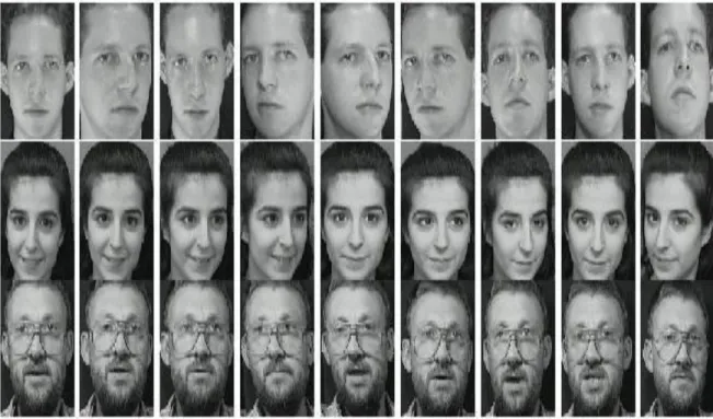
Figure 3.2 Sample images of Yale dataset 34
Figure 3.3 Sample images of LFW dataset. 35
Figure 3.4 Classical face recognition system using The PCA and KNN classifier methods
36 Figure 3.5 Classical face recognition system using the LBPH and KNN
classifier method
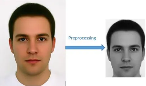
36 Figure 3.6 Example of Prepressing Methods including cropping, resizing
and Histogram
xv
Figure 3.7 Example of the matching case and mismatching case image using KNN with Mahalanobis distance
38
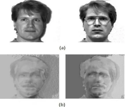
Figure 3.8 An example of PCA (a) Original data. (b) Correlated data 39 Figure 3.9 (a) Original faces (b) Corresponding Eigen-faces 41
Figure 3.10 Original LBP Operator 42
Figure 3.11 Face description with local binary patterns 43 Figure 3.12 Proposed recognition system using PCA and NN classifier
methods
49
Figure 3.13 Proposed recognition system using LPBH and NN classifier method
53
Figure 3.14 The proposed image registration method 54
Figure 3.15 Key-points for Lena with variant threshold. (a) Threshold =100. (b) Threshold =50. (3)Threshold =20
55
Figure 3.16 Matching points with false matching points 55 Figure 3.17 Matching points after eliminating the false points 56 Figure 3.18 Example of image registration. (a) Source and target images
with two matching points. (b) Registered image
56
Figure 3.19 Reference Image. 57
Figure 3.20 The 6 facial landmarks associated with the eye. 58
Figure 3.21 VGGNet model architecture. 59
Figure 3.22 A residual block. 60
Figure 3.23 ResNet50 model architecture. 60
Figure 3.24 Proposed method using a simple CNN. 61
Figure 3.25 Proposed method using VGG16 and VGG19. 62
Figure 3.26 Proposed method using ResNet50. 62
xvi
Figure 4.2 Experiment results using PCA +KNN for ORL data-set 64 Figure 4.3 Experiment results using LBPH + NN for the Yale data-set 66 Figure 4.4 Experiment results using LBPH + NN for the ORL data-set 66 Figure 4.5 Experiment results using PCA + NN with 50% training set and
50% testing set
68
Figure 4.6 Experiment results using LBPH + NN with 50% training set and 50% testing set
69
Figure 4.7 Registration error rate for variant matching point number on Lena image
71
Figure 4.8 Models loss curve. 72
Figure 4.9 Example for registered faces: (a) Original face (b) Predicted registered face (c) Expected registered face.
1
CHAPTER 1: INTRODUCTION
1.1 Research Problem and Scope
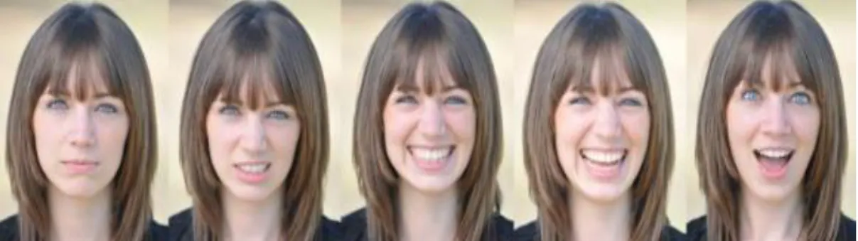
Human face recognition is a challenging task because of the variability of the facial expression, personal appearance, variant poses, and the various illumination as shown in Figure 1.1 [1-4]. Also, due to the variability in lighting intensity, the number of sources, direction, and the camera orientation as illustrated in Figure 1.2, it is a challenging task to design a face recognition system in the real-time with high accuracy recognition rate. Image transformation by rotation, scaling, and a translation is one of the most challenging tasks to solve and has a significant influence on the image recognition as shown in Figure 1.3. The changes in the human face personality should have less effect compared to the pose variation and illumination [5]. Reducing the image dimension is necessary to improve the classification processing time since the object recognition system requires an enormous volume for the computing process. PCA and LBP are one of the popular conventional approaches; both used for robust data representation, as well as histograms, for features reduction [6-13]. Higher accuracy can be achieved by finding a strong representation of the human face by retaining the most dissimilarities in the image data after reducing the dimensionality of the image.
2
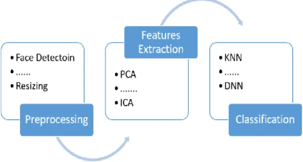
Classical human face recognition systems are divided into three phases as shown in Figure 1.4: The first step is preprocessing, which consists of many types of operations, Figure 1.2.Under variant lighting environments, the face can look different for the same person based on the light source.
Figure 1.1.Same person with variant facial expression.
3
such as image registration, scaling, face normalization, reducing the effect of background noise, detection and resizing, all of which affect the face recognition accuracy. Feature extraction is the second phase, which can be achieved by using powerful transformation approaches. The image dimension can be reduced to a smaller dimension by retaining significant features [12-13]. The final phase is the classification which is using powerful classifiers such as deep neural networks and the fully connected neural networks [14-16]. In this research, we focused on the preprocessing phase and the feature extraction phase which they have a potential improvement.
1.2 Motivation behind the Research
There are many existing algorithms handle the human face recognition. The purpose of these algorithms to achieve an optimal recognition rate or near optimal
4
recognition rate in real-time processing time. However, none of the algorithms achieved a 100% recognition rate. Therefore, human face recognition is an incredibly exciting field for researchers. The neural network classifier is relying on the strong features extraction methods. Neural network performs well with low error rate by feeding strong distinction patterns and features.
This research is motivated by the drawbacks and limitations of existing systems. Existing methods relays on simple preprocessing methods such as face detection and simple image registration. Therefore, we felt that there is a potential improvement can be achieved by implementing a strong image registration based on deep learning approach and a strong features extraction approach which can provide strong distinction patterns and features based on the existing feature extraction methods such as PCA and LBP.
1.3 Potential Contributions of the Proposed Research
In this dissertation, we introduce an enhanced human face recognition framework with a high recognition rate. This improvement based on improving the features extraction approach and improving the image registration based on active shape model deep learning. The proposed framework is suitable for different features extraction methods such as PCA and LBP which we used in this research, and it can be extended to other algorithms such as a deep neural network.
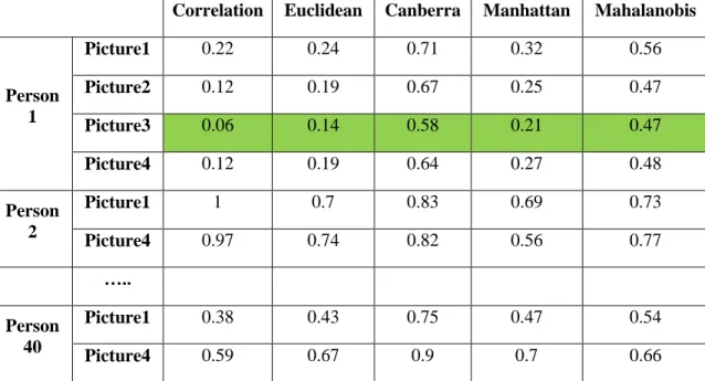
The contribution of the features extraction approach emanated from the first experiment. After we had obtained the training dataset based on the five distance methods, we noticed three scenarios. The first scenario is the optimal matching as shown in Table
5
1.1. All the distance methods were able to find the right match image of the person 1 which is the image 3 of the person 1. The second scenario is partially matching as shown in Table 1.2. Euclidean, Manhattan, and Mahalanobis methods been able to find the right match for person 1 image which was image 2. However, Correlation and Canberra found the wrong match which was the image belong to person 28. The last scenario is the complete mismatching as shown in Table 1.3. All the distance methods failed to find the right image for person 1. Combining the five distance methods using equation (1.1) makes the system more robust and the recognition rate higher since the training dataset will be more significant for the neural network.
√∑
5𝑖=1𝐷𝐼𝑆
𝑖2(1.1)
Table 1.1. The optimal match scenario.
Correlation Euclidean Canberra Manhattan Mahalanobis
Person 1 Picture1 0.22 0.24 0.71 0.32 0.56 Picture2 0.12 0.19 0.67 0.25 0.47 Picture3 0.06 0.14 0.58 0.21 0.47 Picture4 0.12 0.19 0.64 0.27 0.48 Person 2 Picture1 1 0.7 0.83 0.69 0.73 Picture4 0.97 0.74 0.82 0.56 0.77 ….. Person 40 Picture1 0.38 0.43 0.75 0.47 0.54 Picture4 0.59 0.67 0.9 0.7 0.66
6
Table 1.2. The partially match scenario.
Correlation Euclidean Canberra Manhattan Mahalanobis Person 1 Picture1 0.39 0.24 0.71 0.34 0.56 Picture2 0.31 0.14 0.67 0.21 0.36 Person 28 Picture1 1 0.7 0.83 0.69 0.66 Picture2 0.24 0.51 0.71 0.44 0.64 Picture3 0.72 0.54 0.85 0.48 0.79 Picture4 0.4 0.77 0.61 0.56 0.74 ….. Person 40 Picture1 0.41 0.73 0.78 0.41 0.71 Picture4 0.39 0.54 0.92 0.69 0.69
Table 1.3. The complete mismatch scenario.
Correlation Euclidean Canberra Manhattan Mahalanobis
Person 1 Picture1 0.39 0.34 0.71 0.34 0.56 Picture2 0.31 0.32 0.67 0.42 0.49 Picture3 0.41 0.28 0.77 0.29 0.39 Picture4 0.29 0.29 0.64 0.27 0.48 Person 5 Picture3 0.72 0.54 0.85 0.48 0.79 Picture4 0.19 0.77 0.61 0.56 0.32 ….. Person 21 Picture2 0.34 0.41 0.57 0.32 0.74 Person 27 Picture1 0.51 0.57 0.74 0.21 0.64 Person 40 Picture1 0.41 0.27 0.78 0.41 0.71 Picture4 0.39 0.54 0.92 0.69 0.69
7
On the other hand, we are trying to achieve higher accuracy by improving the face registration approach which will lead to a robust end-to-end face recognition system. Since the classical face registration is outdated, we are working on the deep learning based face registration, and we decided to build our deep learning system based on the deep learning concept. We used VGG16, VGG19 and ResNet50 architectures to build our model then we applied the model on one of the State-of-Art datasets such as LFW.
8
CHAPTER 2: LITERATURE SURVEY
The humans can easily and successfully perform face recognition task using their eyes. However, the automatic human face recognition still far from optimal and the researchers with a variant background such as pattern recognition, computer vision, and neural network consider it an area which can be improved. Therefore, the literature survey on human face recognition is diverse. In this survey, a detailed view of the human face recognition methods is presented. Researchers introduced variant algorithms with different accuracy and sometimes inconsistent results comparing to each other. The objective of this survey is to provide an overview of the face recognition process. We focused on the popular categories of feature extraction methods and face registration since the features characterize the whole image [17]. The main purpose of the features extraction is to reduce the image dimension by selecting the most significant features with retaining the relevant information and should be diverse enough among classes for good classification performance. However, the strength of the features extraction methods relies on strong preprocessing approaches like the face registration. The extracted features can be used to classify and to recognize patterns that are present in the source images. Therefore, the face registration and feature extraction process are the key point of the classification performance and thus, in the overall human face recognition.
9
2.1 Preprocessing and Image Registration
Image registration is an essential method used in the image processing systems such as face and object recognition [18-22], object detection, motion estimation [19], and medical application [20]. The information inherited from two related images for the same scene is different. Therefore, they need a proper registration to make the two images uniform and transfer them to the same coordinate system. The classical steps of the image registration are divided into four phases as shown in Figure 2.1 [21]. The first step is to extract the most significant features of the source image and the target image such as edges, corners, and intersections, etc. The key points can be found using methods such as Gaussians difference algorithm [23], segmentation methods [24], representations of general line segments or elongated anatomic structures [25], virtual circles [26], and local curvature discontinuities detected using the Gabor wavelets [27]. These algorithms are recommended if the image contains detectable objects.
On the other hand, the medical images usually have one object and considered as a lake of details. Fast Fourier transform (FFT) used to extract the features in the frequency domain and obtain the parameters based on cross-correlation [28]. The discrete wavelet transform is another method used for feature extraction with root mean square error (RMSE) method [29]. The second step is to find the matching features between the two images from the features which we extracted in step one. Obtaining the corresponding points between the images has been a motivation of many invariant algorithms such as the Scale-Invariant Feature Transform (SIFT) [23], Speeded-Up Robust Features (SURF) [30-32], and Binary Robust Independent Elementary Feature (BRIEF) [33]. Even with these
10
methods, it is still a challenge to obtain the appropriate matches. The RANSAC method is used to eliminate all the mismatching points by finding the best fitting on random subsets of the matches then select the best fitting subset. RANSAC [34] is robust to mismatches but finds a sub-optimal estimation, where LMedS [35] is a more accurate estimation, however, requires at least 50% correct matches. The third step is to find the affine transformation parameters such as translation, scaling, reflection, rotation, and shearing using some of the methods such as the minimized cost function. The last step is transforming the target image to the source image coordinate system using the affine transformation parameters which obtained from the third step.
The researchers moved toward a deep learning based image registration approaches because of the classical image registration limitation. P. Gadde et al. [87] proposed an Image registration with artificial neural networks using spatial and frequency features. In their study, the registration of images is investigated with two novel neural network based approaches, namely, SIFT-DCT and SIFT-DWT. Scale-invariant Feature Transform
(SIFT), Discrete Cosine Transform (DCT), and Discrete Wavelet Transform (DWT) are employed in these approaches. Both new approaches combine features in the spatial domain (SIFT) and frequency domain (DCT or DWT) to provide more robust feature
11
extraction methods for image registration. The learning ability and nonlinear mapping ability of artificial neural network provide a flexible and intelligent tool for data fusion on feature matching and transform model parameter estimation. However, this proposed method obtain the training data using original methods not based on deep learning.
2.2 Feature Extraction for Face Recognition
Feature extraction can be accomplished using numerous mathematical models, image processing techniques, and intelligent computational tools such as neural networks or fuzzy logic. The approaches divided into four categories feature-based, appearance-based, and template-based and part-based approaches as shown in Figure 2.2. In our research, we focused on the feature-based and appearance-based.
Feature Extraction categories
Appearance-based * PCA *LDA *ICA Feature-based * LBP *Gabor Template-based Part-based * SIFT *Component based
12
2.2.1 Appearance-Based Feature Extraction Approach
Appearance-based approaches also known as holistic-based methods identify faces using global features based on the whole image instead of local features of the human face. The new reduced dimension representation of the face obtain by applying some transformation on the entire image. However, the feature-based method obtains the information from some detected fiducial points like eyes, noses, and lips, etc. The fiducial points are usually determined from domain knowledge and discard other information. However, the feature obtained from statistics in the appearance-based methods by performing transformations on the entire face. Holistic-based methods took the most attention against other approaches for the past 3 decades. In this section, we will present an overview of Eigen-face [12] based on the PCA, fisher face based on the LDA, and independent component analysis (ICA). More methods can be found in [36] and [37].
A) Karhunen-Loeve expansion, also known as PCA is one of the popular common approaches, which is wildly used for data representation and features reduction [38]. A solid representation of the human face is achieved by retaining the most variations in the image data after reducing the dimensionality of the image. The concept of the PCA is to translate the human face into a smaller set of features data and keep the variations in the image data-characteristic, which is called Eigen-Faces and they are the principal components of the initial training set of the human face images. The unknown face image in the recognition testing process is projected into a reduced-dimension human face space obtained by the Eigen Faces then classified by distance classifiers or statistical method. Sirovich and Kirby
13
efficiently represent pictures of human faces in 1978 using the PCA. In 1991 Turk and Pentland [12], proposed the popular Eigen-faces method for face recognition. PCA uses the Eigen-Faces to represents human face images as a subset of their Eigen Vectors. Many methods proposed in the computer vision field based on the PCA such as Diagonal PCA [38], and Curvelet-based PCA [39]. Yang et al. [40] proposed Kernel PCA and Kernel FLD for human face recognition, which they called Kernel Fisher-face and Kernel Eigen-face methods. The modular PCA [41] approach has achieved the high accuracy of PCA in cases of extreme change of pose variations, illumination, and expressions. The 2- Dimensional principal component analysis (2DPCA) was introduced as a new approach for feature extraction and representation by Yang et al. [42]. The 2DPCA has numerous advantages over conventional PCA, and it is more straightforward than the PCA to use for face image extraction because 2DPCA regarding the image matrix. Based on Yang method, the 2DPCA is better than conventional PCA in terms of recognition accuracy and is computationally more efficient than conventional PCA therefore; it can improve the process time of image feature extraction significantly. On the other hand, the conventional PCA based image representation is more efficient than the 2DPCA-based image representation regarding storage space because 2DPCA needs more coefficients for face representation.
B) Lu et al. [43] in 2003 and Martinez et al. [44] in 2001 proposed the Fisher‘s linear discriminant analysis (LDA) as a better alternative to the PCA. LDA successfully applied to face recognition area in the past few years. LDA explicitly provides discernment among the classes, while the PCA deals with the input image as entire
14
without paying any attention to the principal structure. The main objective of the LDA is to find a base vector which is providing the best discrimination between the classes to help to maximize the differences between the classes and minimizing the differences within the same classes. The classes are represented by the corresponding scatter matrices Sb and Sw while the ratio is the derivative of | Sb | /| Sw |has to be maximized. LDA outperform the PCA and provide robust
classification performances only when a wide training set is an available base on some results discussed by Martinez and Kak which is confirm this thesis and it called the SSS (Small Sample Size) problem. Belhumeur et al., 1997 considered the PCA as an initial step in order to reduce the dimensionality of the input space then LDA is applied to the resulting space in order to perform the real classification. However, Chen et al., 2000; Yu and Yang, 2001 applied LDA directly on the input space and claimed that combining the PCA and LDA, discriminant information together with redundant one is discarded. Lu et al. (2003) proposed a hybrid between the Direct LDA and the Fractional LDA, a variant of the LDA, in which weighed functions are used to avoid that output classes, which are too close, can induce a misclassification of the input.
C) Generalization of PCA called Independent Component Analysis (ICA) was introduced by Bartlett et al. [45] and Draper et al. [46]. They assumed a better basis of the human face images might be found by methods which are sensitive to these high-order statistics. Moghaddam [47] claimed that the ICA-based approach does not provide a significant advantage over the PCA-based method. Yang [48] showed that the Kernel PCA method outperforms the classical PCA method by
15
applying the Kernel PCA for human face feature extraction and recognition. However, Kernel PCA and ICA are both computationally more expensive than PCA.
2.2.2 Feature-Based Feature Extraction Approach
Feature-based methods exploit more ideas from image processing, computer vision, and domain knowledge from a human face. However, appearance-based methods rely more on statistical learning and analysis. We compared the differences between holistic based methods and feature-based methods and in this section, we discuss two outstanding features for face recognition, the Gabor wavelet feature and the local binary pattern.
A) Local Binary Pattern (LBP) is one of the feature descriptor widely used in face recognition systems. The original LBP operator was introduced by Ojala et al. [49] and was proved a powerful means of texture description. The most important properties of LBP features are the tolerance against illumination changes. LBP is one of the best accomplishment descriptors as it contains the microstructure as well as macro-structure of the face image. Despite its popularity, the LBP approach has some shortcomings, including sensitivity to noise, scale changes, and rotation in the image. The LBP assigns an 18 label to every pixel of an image by thresholding the 3x3-neighborhood of each pixel with the center pixel value, resulting in a binary number [50]. Ahonen et al. [6] applied the LBP on the FERET dataset show good robust performance using one sample per person for training. Besides LBP, other features that widely used in computer vision field can also be used in face recognition, such as fractal
16
features. For example, Komleh et al. [51] presented a method based on fractal features for expression invariant face recognition. Their method is tested on the MIT face database with 100 subjects. One image per subject was used for training while 10 images per subject with different expressions for testing. Experimental results show that the fractal features are robust against expression variation.
B) The Gabor filters represent a powerful tool in image processing and image coding based on the capability of capturing important visual features, such as spatial localization, spatial frequency, and orientation selectivity. In most cases, the Gabor filters are used to extract the main features from the face images. The application of Gabor wavelet for face recognition is pioneered by Lades et al.’s work [52]. They used an elastic graph matching framework to find feature points, build the face model and to perform distance measurement, while the Gabor wavelets are used for extracting local features at these feature points, and a set of complex Gabor wavelet coefficients for each point is called a jet. Lades et al. used a simple rectangular graph to model faces in the database while each vertex is without the direct object meaning on faces. In the database building stage, the deformation process mentioned above is not included, and the rectangular graph is manually placed on each face, and the features are extracted at individual vertices. When a new face I comes in, the distance between it and all the faces in the database are required to calculate, that means if there are totally N face samples are present in the database, we have to construct N graphs
17
for I based on each face sample. This matching process is very computationally expensive, especially for a large database.
2.3 Classification
The simplest method for matching feature vectors is using the nearest neighborhood classifier. It calculates the distance between the source image vector to be classified and the dataset of images vectors, and then assigns the probe the class label of its nearest neighbor in the dataset. If the distance is zero, then the image matched are exactly the same. The distance measure can be converted to a similarity measure simply by negating it, such that the chosen match is the one with the maximum similarity value. The choice of distance metric depends on the type of task, such as Euclidean distance, cosine distance, and chi-square similarity. For an analysis of nearest neighbor pattern classification, see the article by Cover et al. [53]. The advantage of the NN-classifier is that it does not require any training stage and that it naturally extends to multi-class classification. Training other classifiers such as support vector machines (SVM’s) [54] and neural networks [14-16] is often computationally demanding for high-dimensional data with many examples. Even though they may increase matching performance by accounting for non-linearity in the data, training would have to be done every time the gallery is altered.
18
2.4 Neural Network
Computer vision needs powerful classification methods to achieve a high recognition system rate with low computing time and resource. Neural network classification is widely used for training the neural network since NN is simple, efficient to compute the gradient descent, and straightforward to implement. Determine the size of the neural network, the number of samples and the weights is a challenging task, and it is important to fit the neural network output. The NN is divided into three layers which are training input layer, hidden layer (one or more), and the expected output layer as shown in Figure 2.3.
One popular training method is the backpropagation algorithm that uses a gradient descent algorithm [55] to update the parameters of deep learning. In order for gradient descent to map the arbitrary inputs to the target outputs in an accurate manner, gradient descent has to find parameters such as weights 𝑤 and biases 𝑏 that minimize loss function.
19
The input data forward through the network layers to calculate the outputs to compare them with the expected outputs and compute the error of the loss function. The gradient of the loss function computes during the back-forward to update the parameters that minimize the loss function.
The common backpropagation algorithm can be described as the following:
1. The weights 𝑤𝑖𝑗[𝑙] and the thresholds 𝜗𝑗[𝑙], randomly initialize let n=l.
2. Calculate the output of all layers according to equation (2.1) after feeding the prepared training dataset 𝑰𝒑 and the output dataset 𝑶𝒑 to the NN.
𝒚[𝒍+𝟏]𝒋𝒑 = 𝒇(∑𝑵𝟏𝒊=𝟏𝒘[𝒍+𝟏]𝒊𝒋 𝒚𝒊𝒑[𝒍]+ 𝝑𝒋[𝒍+𝟏]) (2.1)
3. In each layer, compute the square root error as follows:
Equation (2.2) used to calculate the square error at the output layer:
𝒆𝒓𝒋𝒑[𝑳]= 𝒇′(𝒏𝒆𝒕𝒋𝒑[𝑳])(𝒅𝒑− 𝒚𝒋𝒑[𝑳]) (2.2)
In the ith hidden layer (i=L-1, L-2 ... i):
𝒆𝒓𝒋𝒑[𝒍] = 𝒇′(𝒏𝒆𝒕𝒋[𝒍]) ∑𝑵𝒍+𝟏𝒆𝒓𝒌𝒑[𝒍+𝟏] 𝒌=𝒍 𝒘𝒋𝒌
[𝒍+𝟏]
(2.3)
4. The change in the weights between the input and the output will be calculated based on equation (2.4) and (2.5).
20
𝒘𝒊𝒋[𝒍](𝒏 + 𝟏) = 𝒘𝒊𝒋[𝒍](𝒏) + 𝜼. 𝒆𝒋𝒑[𝒍]. 𝒚𝒊𝒑[𝒍−𝟏] (2.5)
5. Go back to step 2 if the mean-squared error more than the threshold otherwise stop and print the weight value.
There is many of neuron activation function used in the neural network, and the sigmoidal function is what we used in our proposal system which is shown in equation (2.6).
𝒇(𝒙) = 𝟏
𝟏+𝒆−𝒙 (2.6)
Sigmoidal function derivative is:
𝒇′(𝒙) = 𝒇(𝒙)(𝟏 − 𝒇(𝒙)) (2.7) J. Toms in 1990 improved the backpropagation algorithm using the hybrid neuron because in the big size neural network system was difficult to reach to the minimum mean-squared-error using the sigmoidal activation function compared to the small size neural network which the patterns of the input images are normally classified.
𝒇(𝒙) = 𝝀. 𝒔(𝒙) + (𝟏 − 𝝀). 𝒉(𝒙) (2.8) Where h(x) is the hard-limiting function which is defined in equation (2.9) and the
derivatives of the hybrid neuron is defined in equation (2.10)
𝒉(𝒙) = {𝟏 𝒙 ≥ 𝟎
21
𝒇′(𝒙) = 𝝀𝒔(𝒙)(𝟏 − 𝒔(𝒙)) 𝝀 ≠ 𝟎 (2.10) PBN often trapped into the local minimum and the learning speed is updated according to equation (2.11) where ESS is the Sum-Squared-Error. To make the NN faster and reach to zero error by adding a coefficient α to the steepness of the sigmoidal function as defined in Equation (2.12).
𝝀(𝒏) = 𝒆−𝟏/𝑺𝑺𝑬 (2.11)
𝒇(𝒙) = 𝟏
𝟏+𝒆−𝜶𝒙 (2.12)
Its derivative is:
𝒇′(𝒙) = 𝜶. 𝒇(𝒙)(𝟏 − 𝒇(𝒙)) (2.13) Algorithm (1.1) highlights the essential steps of SGD with mini-batch in iteration 𝑘.
Algorithm 1.1. Stochastic Gradient Descent with mini-batch at iteration 𝑘
1: Input: Learning rate 𝜖 , initial parameters 𝑤, 𝑏 , mini-batch size (𝑚′)
2: While stopping criterion not met do
3: Pick a random mini-batch with size 𝑚′ from the training set (𝑥 (1), … … …., 𝑥 (𝑚))
4: with corresponding outputs 𝑦(𝑖)
5: Compute gradient for 𝑤: 6: Compute gradient for 𝑏: 7: Apply update for: 𝑤 = 𝑤 − 𝜖. ∇𝑤
8: Apply update for: 𝑏 = 𝑏 − 𝜖. ∇𝑏
22
Gradient descent can be categorized into Stochastic Gradient Descent (SGD) and Batch Gradient Descent (BGD). The difference between the two algorithms is how to handle the input data. BGD updates the gradient based on the entire training dataset in each iteration which is considered as a disadvantage, and it could be slow and expensive. However, the convergence is smoother, and the termination is more easily detectable. On the other hand, SGD is less expensive because the gradient computed for each training example and suffers from noisy steps and its frequent updates can make the loss function heavily fluctuate [56].
2.5 Deep Learning Background
Deep learning in the machine learning field achieved numerous performance in the computer vision and the processing of human language applications [57-61]. Deep learning is driven by understanding how the human brain processes information. The brain is organized as a deep architecture with several layers that process the information among many levels of non-linear transformation and representation [62]. Deep learning learns the hierarchy, structure, and pattern of the features from the lower level features using multi-level of hidden layers of non-linear transformations [60]. Very complex functions can be learned with enough such transformations. The higher layers of representation increase aspects of the inputs that are important for discrimination and suppress irrelative variation for any object recognition. For human face recognition, higher layers of representation amplify features of the inputs that are significant for discrimination and subdue irrelative features [63]. The first layer learns the low-level features such as curves, edges, and point from the image pixels. The low-level features are combined in the following layers to
23
produce higher features; for example, points and combined into lines and curves then they combined into shapes and more complex shapes. Once this is done, the deep neural network delivers a probability that these high-level features contain a particular object or scene. The main goal of deep learning is to automatically learn the most discriminative features from the raw data without human involvement. Convolutional Neural Networks (CNN) Stacked Auto-encoder (SA), Recurrent Neural Network (RNN), and Deep Belief Network (DBN) are the popular models for deep learning. [64, 65].
2.6 Convolutional Neural Network
CNN is a class of deep, feed-forward artificial neural networks, most commonly applied to analyzing visual imagery that takes advantage of the spatial construction of the inputs. A CNN consists of an input and an output layer, as well as multiple hidden layers.
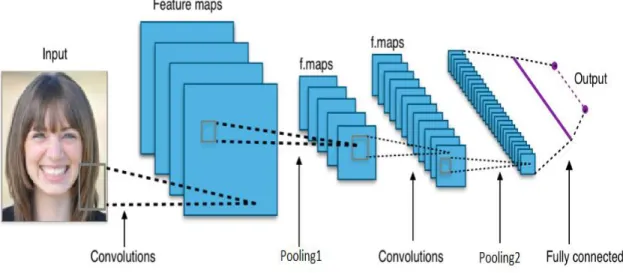
CNN consist of alternating convolutional layers followed sometime by pooling layers and dropout layers to avoid the overfitting issue. The network end with few of fully-connected layers followed by classifier layer such as soft-max classifier or regression classifier as shown in Figure 2.4.
The CNNs gain the advantage by learning features representation automatically without depending on human-crafted features using end-to-end system starting from raw pixels to classifier outputs [61, 66]. Since 2012, researchers focus on improving the performance of CNNs architecture and methods such as layer design, activation function, and regularization, and exploring the performance in different fields [67, 68]. Resnet50,
24
Inception v4 and FaceNet are some of the existing models which they can be used to train a dataset on different domain issue.
2.6.1 Convolutional Layer
The convolutional layer is the core building block of a CNN. The convolutional layer's parameters comprised of a set of learnable kernels (or filters). The convolutional layer extracts local features from the input by sliding a filter over the input and computing the dot product and producing a 2-dimensional activation map of that filter as shown in Figure 2.5. The feature maps connected to a small region of the input called receptive field, and the new feature map is generated by convolution operation and followed by a non-linear activation function as shown in Equation (2.14) to introduce non-non-linearity into the model. 𝑥𝑓(𝑙) = 𝑓(∑ 𝑥(𝑙−1) 𝑆,𝑆 ∗ 𝑤𝑓 (𝑙)+ 𝑏 𝑓 (𝑙) ) (2.14) Figure 2.4. The typical structure of a CNN.
25
Where the f is non-linear activation function, 𝑏𝑓(𝑙)is shared bias of the feature map, 𝑥(𝑙−1) is the output of the previous layer, * is convolution operation, and 𝑤
𝑓 (𝑙)
is convolution filter with size S × S.
CNN compute the gradient of the loss function with respect to the weights (𝑤) and biases (𝑏) of the respective layer in the backward phase as follows:
∇𝑤𝑓(𝑙)𝑙 = ∑ (∇x𝑓(𝑙+1)𝑙) 𝑆,𝑆(𝑥𝑆,𝑆 (𝑙) ∗ 𝑤𝑓(𝑙)) 𝑆,𝑆 (2.15) ∇𝑏𝑓(𝑙)𝑙 = ∑ (∇x𝑓(𝑙+1)𝑙) 𝑆,𝑆(𝑥𝑆,𝑆 (𝑙) ∗ 𝑏𝑓(𝑙)) 𝑆,𝑆 (2.16)
All units share the same weights (filters) among each feature map. The advantage of sharing weights is the reduced number of parameters and the ability to detect the same feature, regardless of its location in the inputs [69]. The hyper-parameters of each convolutional layer must be chosen carefully in order to generate desired outputs such as e filter size, the number of learnable filters, and stride.
Numerous nonlinear activation functions are existing, such as sigmoid, tanh, and ReLU. However, ReLU is preferable because it makes training faster relative to the others [70, 71]. The filter size and stride decides the output features map size (WxW) based on the input image with a size of (H × H) over a filter with a size of (F × F) and a stride of (S) as:
𝑊 = ⌊𝐻−𝐹
26
2.6.2 Pooling Layer
Typically the pooling layers (down-sampling layer) applied after the convolutional layers to reduce the resolution of the previous feature maps and preserve most relevant feature. Pooling provides a fixed size output, which is important for classification. Pooling produces invariance to a small transformation and/or distortion. Pooling splits the inputs into disjoint regions with a size of (R × R) to produce one output from each region [72]. Two pooling are exist: Max-pooling and Average-pooling and the output size will be obtained from the input with a size of (W × W) by:
27 𝑃𝑜𝑜𝑙𝑖𝑛𝑔 = ⌊𝑊
𝑅⌋ (2.18)
We are losing global information about locality, and where in image something happened by applying a max-pooling in CNN [55, 73]. However, we are keeping information about whether the most important feature appeared in the image or not.
The maximum value of non-overlapping blocks from the previous feature map (𝑙−1) is calculated during the forward phase as follows:
𝑥(𝑙) = 𝑚𝑎𝑥𝑅,𝑅(𝑥(𝑙−1))
𝑅,𝑅 (2.19)
There are no any learnable parameters in the Max pooling. Therefore, the gradient from the next layer is passed back only to the neuron that achieved the max value and all of the other neurons receive zero gradient. Figure 2.6 shows how the max-pooling works.
28
2.6.3 Fully Connected Layer
The CNN ends with one or more of the fully connected layers that connect every neuron in one layer to every neuron in another layer and has the only number of neurons hyper-parameter. It is in principle the same as the traditional multi-layer perceptron neural network (MLP). Fully connected layer purpose is to extract the global features of the inputs, and the output is computed by Equation (2.20):
𝑥(𝑙) = 𝑓((𝑤(𝑙))𝑇. 𝑥(𝑙−1)+ 𝑏(𝑙)) (2.20)
Where is the (𝑙), (𝑙), and (𝑙) are the input, weights, and biases of the current layer (l), x (l-1) is the output of the previous layer, is a dot product, and 𝑓 is the non-linear activation function. The last layer is the classifier layer such as soft-max classifier and regression classifier.
2.7 Literature Review for Face Registration
2.7.1 Speed-Up Robust Features (SURF)
The Speeded-up Robust Features (SURF) is a method to obtain the local features which will be used to align two related images which are taken at a different time or a different position. SURF process includes feature detection, feature description, and feature matching. The SURF steps are:
1) Find the integral image (IΣ) based on the input image I to achieve fast computation of the convolution filters. The value for each point P =(x, y) is represented by the sum of all pixels in the input image I. Then we calculate the
29
sum of the intensities within a rectangular region formed by the origin and P using equation (2.21).
𝛴 = 𝐼𝛴(𝐶) − 𝛴(𝐵) − 𝛴(𝐷) + 𝛴(𝐴) (2.21) 2) Find the interesting points using hessian matrix by finding the maximum
hessian matrix corresponding to a point P =(x, y).
3) Subtract the adjacent Gaussian images to obtain the difference of Gaussian images by repeatedly convolved with Gaussians.
4) Optimize the key-points after obtaining image gradients using three methods to obtain the descriptor.
5) Finding the orientation Assignment: using the pixel differences, we compute orientation θ(x, y) and gradient magnitude M(x, y) for each image sample L(x,
y).
𝑀(𝑥, 𝑦) = √𝐴2+ 𝐵2 (2.22)
6) Obtaining Key-point descriptors: 64 element vector obtain by combining all the orientation histogram entries.
7) Perform the k-nearest-neighbor (KNN) on the feature values to find the distance between the features using four steps:
i. Compute the Euclidean distance on the obtained features. ii. Descending sort of the labeled example.
iii. Based on root mean square deviation (RMSE), find the optimal K of the KNN.
30
2.7.2 Minimized Cost Function
Matrix equation (2.23) is used to minimize the cost of the image registration (without shear) when the related points in two images X and Y are identified. Summation indicates the sum over all points in an image. We used in our implementation the sigmoidal function as the neuron activation functions.
(2.23)
To find the optimal transformation that will align image 2 to image 1, take the partial derivatives of the above cost with respect to a, b, t1 and t2 and set these to 0 (∂C/∂a = 0, ∂C/∂b = 0, ∂C/∂t1 = 0, ∂C/∂t2 = 0). We express the four resulting equations in matrix form as is shown in equation (2.24).
(2.24)
After calculating the sum over all points for the 4x4 matrix and the right-hand 4x1 vector in equation (2.24), we can compute the required transformation by:
Matrix Ainv = A.Inverse and Matrix Res = Ainv * B.
2.7.3 Random Sample Consensus (RANSAC)
Fischer et al. introduced the RANSAC algorithm in 1981. RANSAC is one of the most suitable algorithms to eliminate the false matched points in the source and target
31
images in the presence of noise [17]. Some of the disadvantages of RANSAC are computing time, correct matches count, and the dependency of mismatches removal on the amount of threshold value. RANSAC algorithm is divided into four steps. The first step is to select a suitable model based on the transformation model. Equation (2.25) is used to calculate the number of related points which are required to calculate the transformation parameters. q is the minimum number of the related points and p is the number of the parameters need to calculate.
𝑞 =𝜌
2 (2.25)
The second step is selecting the best model in a specified iterations. In each iteration, the minimum number of the related points randomly selected to estimate the transformation parameters based on equation (2.26) for 6 parameters a, b, c, d, e, and f.
(2.26)
The third step is to calculate the distance between the source image and the transformed image. We consider a point is a right match if the distance is less than the threshold. Otherwise, we eliminate the point since it is not a true match. In the last step, for each iteration, we count the numbers of the true match, and if they are more than the desired value, or reaches the predetermined maximum number of iterations, then the algorithm stops. Transformation model selected which has the highest matching count.
32
CHAPTER 3: RESEARCH PLAN AND SYSTEM
ARCHITECTURE
This research aims to achieve a higher human face recognition with less computation processing time. Image registration and feature extraction are the key points of improving face recognition. Therefore, we implemented our system based on multiple classification methods. To compare our results with the existing face recognition systems, we applied our frameworks on two of the well-known human face image databases, Yale and Olivetti Research Laboratory Human Face Datasets. We implemented some of the existing face recognition systems to compare our testing results to their results. We randomly obtain the training set and the testing set with different scenarios. Different size of dataset applied to like 90% of the picture as training and 10% as a testing set or 70% to 30%. Our goal is to achieve higher accuracy of the 50% to 50% scenario. Finally, recognition rate (RR) is calculated using equation (3.1) after the system finishes training the NN then test the testing set.
𝑅𝑅(%) =
𝑁𝑢𝑚𝑏𝑒𝑟 𝑜𝑓 𝑐𝑜𝑟𝑟𝑒𝑐𝑡 𝑚𝑎𝑡𝑐ℎ𝑁𝑢𝑚𝑏𝑒𝑟 𝑜𝑓 𝑡𝑟𝑎𝑖𝑛𝑖𝑛𝑔 𝑠𝑒𝑡
*100
(3.1)3.1 Human Face Datasets
3.1.1 ORL Dataset
Olivetti Research Laboratory Dataset (ORL) [74]. ORL dataset represents images of 40 different persons with ten different pictures for each person. A total of 400 face
33
images used for training and testing the system. The 400 images are in grayscale, and the size is 92X112 pixels with variant expressions, timing, pose, and gender. Figure 3.1 shows a sample of the ORL dataset.
3.1.2 Yale Dataset
The Yale face dataset has a total of 165 face images which represent 15 different persons with 11 images per person [75]. Different facial expression, gender, light configuration, and with or without wearing eyeglasses. The 165 images are in a grayscale
34
domain and images resized to 92x112 pixels after we cropped the face only. Figure 3.2 shows Yale sample images.
3.1.3 Labeled Faces in the Wild
The data set contains more than 13,000 images of faces collected from the web. Each face has been labeled with the name of the person pictured. 1680 of the people pictured have two or more distinct photos in the data set. The only constraint on these faces is that they were detected by the Viola-Jones face detector. The images are in color scale, and the size is 250x250 pixels with variant expressions, timing, pose, and gender. Figure 3.3 shows a sample of the LFW dataset.
3.2 Classical Face Recognition System
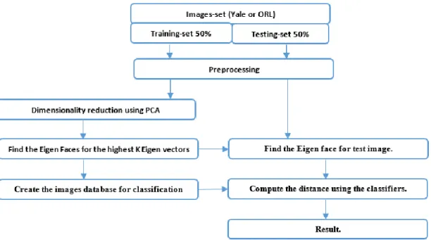
We implemented the classical face recognition system as a baseline for our research. First, we used the PCA and the KNN classifier [1] only as shown in Figure 3.4.
35
The goal of the PCA is to reduce the face image dimension by using only the highest K Eigen-values and their corresponding Eigen-vectors with losing minimal information, which helps to reduce the computation process. Second, we used LBPH and the KNN classifier as shown in Figure 3.5. The goal of the LBPH is to reduce the face image dimension by dividing the image into small regions called cell and represent each cell by 59 dimensions with losing minimal information. We used five different distance classifiers to measure the similarity between the source image and the test image to show how accuracy is different between the methods, which lead us to combine them in the proposed framework to achieve higher accuracy.
36
Figure 3.4. Classical face recognition system using The PCA and KNN classifier methods.
37
We reduced the computation time in both frameworks by preprocessing the face images using different methods as needed. The preprocessing starts with resizing the image to a reasonable size followed by cropping the face only to eliminate the face background effect. Reducing the noise and the illumination by converting the face images to grayscale images and histogram equalization to build a robust face recognition system, Figure 3.6 shows some of the preprocessing methods. The new face representation is obtained from the PCA or the LBPH which present the face image in a smaller dimension. Finally, using one of the classifier measurements we calculate the similarity between the source image and the target image and we consider the matching occurs only if the lowest KNN neighbor matches the source as shown in Figure 3.7(a) otherwise it will be considered as a mismatch as shown in Figure 3.7(b). Then, we calculate the recognition rate for the whole system using equation (3.1).
38
3.2.1 Principle Component Analysis
Image recognition and detection need a massive resource of storage and powerful system to reduce the computation processing time and cost. Therefore, the dimension reduction and image re-representation are needed as the first step in any face recognition systems. PCA is one of the popular statistical transform methods. PCA reduces the image dimension by analyzing the image and identifying distinction patterns which can be used as a new representation of the image without losing an enormous information content from the image. Face dimension reduction is obtained by applying the PCA and finding the highest K Eigen-Values and their corresponding Eigen-Vectors. The face image can be re-represented using only 15% of the Eigen-Values with a minimal losing of information [76]. PCA is relying on the variance-covariance matrix. Therefore, the images are not a significant comparison to the number of face images in the training dataset. The advantages Figure 3.7.Example of the matching case and mismatching case image using KNN with Mahalanobis
39
of the PCA are low noise sensitivity, eliminating the data redundancy by providing the orthogonal components and reducing the image complexity. The disadvantages of the PCA methods are evaluating the variance-covariance matrix and capturing the invariance. Evaluating the variance-covariance matrix in an accurate manner and capturing the invariance is difficult unless the training dataset explicitly provides the information. Figure 3.7 shows an example of the PCA methodology. Figure 3.8(a), the face data are randomly distributed, and Figure 3.8(b) shows the correlated data grouped in the same coordinate face space.
The PCA process starts with standardizing the image scale by obtaining the same face size vector 𝛤𝑖 for all of the training images I1, I2… IM. The training data-set of M faces written as I = (I1, I2, IN) and the average image 𝛹 is obtained by equation (3.2).
𝛹 = 1
𝑀∑ 𝛤𝑖 𝑀
𝑖=1 (3.2)
40
Then centralize each training image by subtracting the mean, which is the average across all dimensions from each image and finds the vector 𝛷 = 𝛤𝑖 − 𝛹𝑖 . PCA uses equation (3.3) to calculate the covariance-matrix C, which is used to find the Eigen-Value.
𝐶 = 1 𝑀∑ 𝛷𝑚𝛷𝑚 𝑇 𝑀 𝑀=1 = 𝐴𝐴𝑇 (𝑀2𝑥𝑀2 𝑚𝑎𝑡𝑟𝑖𝑥) (3.3) 𝑊ℎ𝑒𝑟𝑒 𝐴 = [Φ1Φ2… … … Φ𝑀] (𝑁2𝑥𝑀 𝑚𝑎𝑡𝑟𝑖𝑥).
We can calculate the Eigen-Values 𝜇𝑖 and the Eigen-Vectors 𝑣𝑖 from the covariance matrix since the matrix is square using equation (3.4).
𝐴𝑇𝐴𝜈𝑖 = 𝜇𝑖 𝜈𝑖 (3.4) PCA significantly orders the Eigen-Values from highest to lowest. We then ignore low significance Eigen-Values to reduce the face domain, and we obtain the corresponding Eigen-Vectors. PCA loses some of the information from the image. However, this will not affect the recognition since most of the data discrepancy exists in the first 15% of the face dimension. We obtain the Eigen-Faces by transpose the Eigen-Vectors then multiply them by the original faces dataset. Eigen-Faces appears as ghostly faces in Figure 3.9.
Eigen-Faces = (Original data-set) X (Eigen-Vectors)
3.2.2 Local Binary Patterns Histogram (LBPH)
Correlation methods require substantial computation time and enormous amounts of storage. Therefore, features reduction and face representation are needed in the face recognition system. LBPH is usually a preferred method in computer vision, image processing, and pattern recognition; it is appropriate for the feature because it describes the texture and structure of an image. We represent the face image and reduce the image
41
dimension by applying the LBPH method, extracting the features texture of the image by dividing the image into local regions and extracting the binary pattern for each local region. The original LBP operator, which works on eight neighbors of a pixel, was introduced by Ojala et al. [49]. The image is divided into small regions called the cell. Each pixel in the cell is compared with each of its eight neighbors. The center pixel value will be used as the threshold value [6-11]. The eight-neighbors-pixel will be set to one if its value is equal to or greater than the center pixel; otherwise, the value is set to zero. Accordingly, the LBP code for the center pixel is generated by concatenating the eight neighbor pixel values (ones or zeroes) into a binary code, which is converted to a 256-dimensional decimal for convenience as a texture descriptor of the center pixel. The original LBP operator is shown in Figure 3.10.
42
The mathematical formulation of LBP operator is given by:
𝐿𝐵𝑃(𝑥) = ∑8 𝑠(𝐺(𝑥𝑖
𝑖=1 ) − 𝐺(𝑥))2𝑖−1 (3.5)
𝑠(𝑡) = {1 𝑡 ≥ 0
0 𝑡 < 0 (3.6)
We used a modified LBP operator called a uniform pattern. The pattern is the number of bitwise transitions from 1 to 0 or vice versa. The LBP is called uniform if its uniformity measure is at most 2. For example, the patterns 11111111 (0 transitions), 01111100 (2 transitions) and 11000111 (2 transitions) are uniform, while the patterns 10001000 (3 transitions) and 11010011 (4 transitions) are not. For dimension reduction, we used the histogram to reduce the image features from a 256-dimensional decimal to a 59- dimensional histogram, which contains information about the local patterns. The histogram uses a separate bin for each uniform pattern, and one separate bin for all non-uniform patterns. In the 8-bit binary number, we have 58 non-uniform patterns; therefore, we
43
used 58 bins for them and one bin for all non-uniform patterns. The global description of the face image is obtained by concatenating all regional histograms. The overall value of LBPH can be represented in a histogram as (3.7):
𝐻(𝑘) = ∑𝑛𝑖=0∑𝑚𝑗=1𝑓(𝐿𝐵𝑃𝑃,𝑅(𝑖, 𝑗), 𝑘), 𝑘 ∈ [0, 𝑘] (3.7) Where P is the sampling points, and R is the radius.
Figure 3.11 shows the process of getting the feature vector for each image, which will be fed to the classifier.
3.2.3 Similarity Measurements Methods
The K-Nearest-Neighbors (KNN) is one of the methods used in the computer vision. Most of the KNN use the Euclidean distances. However, it produces less accurate results than the other methods. Each distance method provides different levels of accuracy based on the problem domain. Therefore, the first contribution is to combine some of them
44
to improve the face recognition accuracy. Mahalanobis distance measurement provides more accurate result than Minimum Distance depending on the covariance matrix between the two vectors in the (3.8) [77].
Mahalanobis(x, y)=√(xi − yi)TS−1(xi − yi) (3.8)
Where 𝑺−𝟏 is the covariance matrix inverse.
Correlation distance classifier was introduced by Székely, Rizzo, and Bakirov in 2007 [78]. A valuable property is the measure of dependence equal zero and is sensitive to a linear relationship between two vectors.
Correlation(x, y) =Cov(x,y)σ
x σy (3.9)
Where Cov is the covariance and 𝛔𝐱 and 𝛔𝐲 are the standard deviations of x and y.
Euclidean distance method is consideredthe basis of many measures of similarity and dissimilarity. We use (3.10) to calculate the Euclidean distance between corresponding elements of the two vectors space.
Euclidean(x, y) = √∑M (xi − yi)2
i=1 (3.10)
The Canberra distance classifier is a numerical measure of the distance between two points in a vector space, which is presented in (3.11):
45
The Manhattan distance classifier is another method to measure the distance between two vectors and is introduced in (3.12):
Manhattan(x, y) = ∑M |xi − yi|
i=1 (3.12)
We used different distance classifier methods to provide a variant dataset to improve the training of the neural network.
3.3 Face Recognition using PCA and NN Proposed System
3.3.1 Proposed Method
We proposed in this paper an enhanced Face Recognition Framework Based on Correlated Images and Back- Propagation Neural Network. The main contributions of our work are:
Using five distance methods and combining them will provide a clear pattern which helps the NN to converge faster and more accurate.
Obtaining the T-Set based on the correlation between the training dataset will provide robust data which we used as an input of the NN.
Each distance method performs well in a different direction. Therefore, adding a strength factor helps to improve the accuracy rate.
The proposed framework is divided into five steps as shown in Figure 3.12
1) Preprocessing step: Face recognition needs huge storage and CPU resources. Therefore, we applied a few of the preprocessing operations to reduce the computing time as shown in Figure 3.5. Haar-cascade
46
detection is used to detect the face then we cropped the face to reduce the background effect. We converted the images to a gray-scale image then we applied a histogram equalizer to reduce the noise effect. Finally, we resized the images to the size we preferred.
2) Features extraction: We used the PCA algorithm to reduce the dimensionality of the images by eliminating the redundant data between the training images while retaining the variation between them. The PCA is transforming the dataset into a new set of variables which called the principal components (PCs). The first PC retains the maximum variation in the dataset. The PCA sorts the Eigen-Vectors and selects to top K values to reduce the dimensions. The training dataset