Multi-Sensor Fusion for 3D Object Detection

(1)

Rochester Institute of Technology Rochester Institute of Technology

RIT Scholar Works

Theses

6-2020

Multi-Sensor Fusion for 3D Object Detection

Darshan Ramesh Bhanushali

[email protected]

Follow this and additional works at: https://scholarworks.rit.edu/theses

Recommended Citation Recommended Citation

Bhanushali, Darshan Ramesh, "Multi-Sensor Fusion for 3D Object Detection" (2020). Thesis. Rochester Institute of Technology. Accessed from

This Thesis is brought to you for free and open access by RIT Scholar Works. It has been accepted for inclusion in Theses by an authorized administrator of RIT Scholar Works. For more information, please contact

(2)

Multi-Sensor Fusion for 3D Object Detection

By

Darshan Ramesh Bhanushali

June 2020

A Thesis Submitted in Partial Fulfillment

of the Requirements for the Degree of Master of Science

in

Computer Engineering

Committee Approval:

Dr. Raymond Ptucha, Advisor Date

Associate Professor

Dr. Amlan Ganguly, Committee Member Date

Associate Professor

Dr. Clark Hochgraf, Committee Member Date

Associate Professor

(3)

2 | P a g e

Acknowledgments

I would like to take this opportunity to thank my advisor Dr. Raymond Ptucha for his support and guidance throughout my master’s degree. I am thankful for Dr. Amlan Ganguly and Dr. Clark Hochgraf for being on my thesis committee. I would also like to thank my parents, my sister Bhakti and my friends; without their support this journey would not have been as joyful as it was. I would like to thank Dr. Michael Kuhl and my friend Samrat Patel for their advice and suggestions. I am indebted to the iMHS team for all the support and discussion sessions.

(4)

3 | P a g e

Abstract

Sensing and modelling of the surrounding environment is crucial for solving many of the problems in intelligent machines like self-driving cars, autonomous robots, and augmented reality displays. Performance, reliability and safety of the autonomous agents rely heavily on the way the environment is modelled. Two-dimensional models are inadequate to capture the three-dimensional nature of real-world scenes. Three-dimensional models are necessary to achieve the standards required by the autonomy stack for intelligent agents to work alongside humans. Data driven deep learning methodologies for three-dimensional scene modelling has evolved greatly in the past few years because of the availability of huge amounts of data from variety of sensors in the form of well-designed datasets. 3D object detection and localization are two of the key requirements for tasks such as obstacle avoidance, agent-to-agent interaction, and path planning. Most methodologies for object detection work on a single sensor data like camera or LiDAR. Camera sensors provide feature rich scene data and LiDAR provides us 3D geometrical information. Advanced object detection and localization can be achieved by leveraging the information from both camera and LiDAR sensors. In order to effectively quantify the uncertainty of each sensor channel, an appropriate fusion strategy is needed to fuse the independently encoded point clouds from LiDAR with the RGB images from standard vision cameras. In this work, we introduce a fusion strategy and develop a multimodal pipeline which utilizes existing state-of-the-art deep learning based data encoders to produce robust 3D object detection and localization in real-time. The performance of the proposed fusion model is evaluated on the popular KITTI 3D benchmark dataset.

(5)

4 | P a g e

List of Figures

Figure 1 Basic framework of an autonomous agent. 8

Figure 2 Human perception and machine interpretation of the image. 16

Figure 3 Visualization of a point cloud obtained from LiDAR along with

corresponding left RGB camera image.

17

Figure 4 Multi-view RGB(D) image rendered from a point cloud. 17

Figure 5 LiDAR point cloud overlaid on corresponding camera image. 19

Figure 6 An example of 2D convolutions. 21

Figure 7 A typical CNN architecture consisting of multiple consecutive layers of convolution and max pooling operations.

22

Figure 8 Overview of skip connections in deep networks. 23

Figure 9 Overview of VGG19 architecture and ResNet34 architecture. 24

Figure 10 Different residual units. 26

Figure 11 Overview of the PointNet architecture. 27

Figure 12 Overview of the VoxelNet. 28

Figure 13 Effect of different γ value on focal loss. 31

Figure 14 Plot of smoothL1 loss. 32

Figure 15 Overview of the Pointpillar architecture. 34

Figure 16 Simplified PointNet Architecture. 35

Figure 17 Architecture overview of the proposed Early Fusion network. 38

Figure 18 Effect of Average Filter. 39

Figure 19 The architecture overview of the proposed Late Fusion network. 40

Figure 20 ResNet like CNN architecture for image feature extraction. 41

Figure 21 Overview of the Combined Fusion network. 42

Figure 22 Sensor placement scheme of the car used to collect KITTI dataset. 44

Figure 23 An example from the KITTI dataset. 45

(8)

7 | P a g e Figure 25 BEV and 3D object detection performance vs Kernel size of the

average filter.

(9)

8 | P a g e

List of Tables

Table 1 Sizes of output and convolutional kernels for different variants of ResNet.

25

Table 2 Thresholds for difficulty levels of the annotations. 43

Table 3 Configuration setup for Baseline, Early fusion, Late Fusion and Combined Fusion model.

48

Table 4 3D detection benchmark scores. 49

Table 5 BEV detection benchmark scores 50

(10)

9 | P a g e

Chapter 1

Introduction

1.1

Introduction

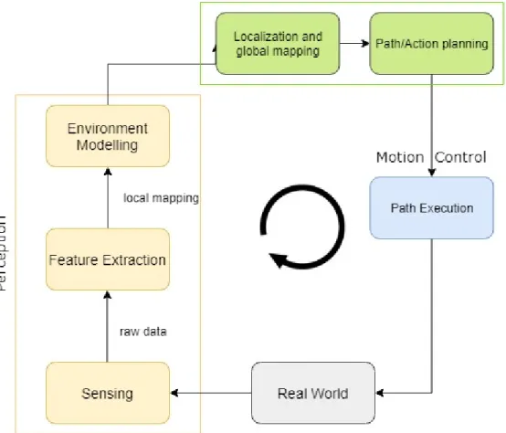
Object detections plays an important role in many applications where environment perception is needed such as autonomous vehicles, autonomous robots, and augmented/virtual reality. Figure 1 shows a typical framework of an autonomous intelligent agent. The framework consists of environment perception, self-localization, path planning and motion control. Safe interaction of such autonomous systems with the surrounding environment and humans is highly dependent on its ability to detect, perceive and model its environment.

(11)

10 | P a g e A lot of progress has been made in 2D object detection, but the progress in 3D object detection has been a difficult challenge. The world around us is in 3D form and 3D perception can ensure the critical safety needs of the autonomous machines and robots. Robustness and real-time inference are the two major requirements for such 3D object detectors. Given the list of particular objects to be detected, the task of 3D object detection (3DOD) is defined as a task in which a machine is able to identify those objects in the scene as well as localize the relative position of those objects in 3D space.

LiDAR and camera are the two most useful sensors for environment perception. Cameras provide detailed texture and color information of the object’s surface and LiDAR provides 3D geometrical information of the objects shape as well as the relative distance of the object from the sensor. The challenge in 3D object detection is because neither of those sensors alone can provide enough information to be able to achieve robust output for real world applications. One of the current bottlenecks in the field of multi-modal 3D object detection is the fusion of 2D data from the camera with 3D data from the LiDAR.

Modelling the LiDAR and camera sensor data is the first crucial element of a 3DOD architecture. Encoders based on neural network architectures like Convolutional Neural Network (CNN) [1] and PointNet [2] have proven to be very efficient and effective in modelling the high dimension sensor data to a compressed lower dimensional vector. Availability of large amount of 3D annotated and synchronized LiDAR-camera data in the form of well-designed datasets such as KITTI [3], Waymo Open Dataset [4], nuScenes [5], and Lyft Level 5 AV Dataset 2019 [6] have accelerated the research in data driven 3D deep learning-based object detectors. The second element of 3DOD is classification of these vectors to identify and detect the object and its relative position. The efficiency of classification depends greatly on efficiency of the encoder.

The point clouds obtained from a LiDAR are usually irregular and sparse over the space, hence most researchers transform them into either fixed sized voxel grids [7, 8, 9, 10] or project them on a 2D surface to obtain a bitmap image [11, 12, 13, 14]. CNN based encoders can capture information for 2D images, but they do not perform well on sparse

(12)

11 | P a g e sensor data like point clouds [8, 13, 15]. A network based on point cloud 3D convolution can generalize better, is more suitable for transfer learning applications, and is able to hold the permutation invariance of the points in the input. Hence arises a need for a separate and parallel encoder networks for different modalities and then using an efficient fusing method to combine and weigh the information from each sensor modality to build an accurate model of the surrounding environment. Pointpillar [7] has demonstrated better results with just LiDAR based network as compared to fusion based methods. Hence more work is needed to fuse multimodal data in a principled manner for developing efficient multimodal fusion based networks.

1.2

Motivation

The general motivation behind 3DOD research is the fact that the 3DOD task is still an unsolved problem with scope for improvement in numerous areas like speed of inference, memory requirement, accuracy and most importantly robustness and safety. 3DOD is an important part of the autonomy stack in making it safe and more efficient. Currently, 2DOD provides adequate information for implementing some of the simpler tasks required in advanced driver assistance like adaptive cruise control, and emergency braking. Fully autonomous mobile robots and vehicles require performing much more complex tasks like efficient path planning, complex maneuvers, and lane changing, which require 3D understanding of the environment to plan and make decisions.

There has been a lot of efforts and development in single input modality models for 3DOD task achieving great results. Fusion of LiDAR-camera data for real-time 3DOD has several technical challenges. Camera images can be processed using CNNs while LiDAR pointclouds can be processed by using PointNet [2] and other graph-based networks. The typical region proposal networks [16, 17] (RPN) used in image-based object detection pipelines are not suitable for pointcloud and image data fusion-based networks. Fusion from the two data sources can be done at different levels in the architecture.

(13)

12 | P a g e Multi-modal fusion-based networks can lead to more robust models which are less prone to sensor failures, occlusions, and challenging capture conditions such as nighttime or rain. Each fusion strategy has its own properties that pose challenges to deep architecture design while providing the opportunity for novel and efficient solutions.

This thesis aims at developing a multi-modal fusion based 3D object detector which leverages environment perception data obtained from both LiDAR and camera sensor to provide robust and accurate detections. Such a detector can be used for 3D object detection for indoor as well as outdoor environments. We evaluate the performance of the network using KITTI 3D object detection benchmark dataset [18].

1.3

Contributions

This thesis focuses on developing better fusion strategies using the existing state of the art encoders to perform time 3D object detection and localization. We consider a real-time model as defined as being able to process 10 frames per second or more. This thesis experiments with different sensor fusion strategies based on the stage of the network at which the information fusion is incorporated, specifically early fusion, late fusion and combined fusion. We analyze the effect of each fusion strategy and their respective parameters to be tuned quantitatively and qualitatively. In this thesis, we introduce advantages and disadvantages for each of the fusion strategies. We discuss on how to encode the sensor data as neural network input and output, and key tuning parameters for designing the corresponding fusion network architecture.

• We evaluate the three fusion strategies using the KITTI 3D Object Detection Benchmark Dataset and discuss their results on both Bird’s Eye View (BEV) and 3DOD tasks for cars, pedestrian, and cyclists.

• The main contribution of this work is a novel multimodal fusion based pipeline for LiDAR-camera data called combined fusion network that offers enhanced 3D detection over prior methods. The proposed fusion network is an end-to-end learn-able network that incorporates early as well as late fusion. We also discuss the key tuning parameters of the resulting fusion network.

(14)

13 | P a g e • We perform several ablation analyses to look at the main factors that allow strong

(15)

14 | P a g e

Chapter 2

Background

In this section, we present a theoretical background regarding the data structure, algorithms, loss functions, sensors and other relevant subjects involved in this thesis project. Section 2.1 describes the various possible data structures which can be used to represent data from camera and LiDAR. In Section 2.2, various concepts related to data fusion for different sensors are described. Section 2.3 introduces neural networks such as Convolutional Neural Network and PointNet which are required for processing camera and LiDAR data respectively.

2.1

Sensor Modalities and Data Representations

Data representation refers to the format in which the sensor data is stored on the computer. Different data have different representation for efficient storage and retrieval. Each data type has its own pros and cons in terms of storage, ease of algorithmic analysis and inference speed.

2.1.1

Camera

A camera provides visual data of the surrounding by capturing the incident light in the form of images or sequence of images (video). It is widely available and relatively inexpensive compared to other sensors like LiDAR, RADAR, and stereo cameras. It provides rich texture and color information of the vehicle surround in real time (15Hz - 120Hz) but lacks depth information. An image frame from the camera can be represented in the form of dense 2D array with each element (pixel) of the array containing the corresponding pixel intensity. The pixel information can be encoded in different forms like RGB, HSV, or grayscale. Due to the lack of depth information, inferring 3D geometry using 2D camera data is challenging. Figure 2 shows a cropped image from KITTI dataset [3] and its machine interpretation.

(16)

15 | P a g e Figure 2: Human perception (left) and machine interpretation (Right) of the image.

2.1.2

LiDAR

Unlike camera, LiDAR provides a 3-dimensional point cloud of the surrounding environment, thus providing data rich in depth information but lacks color and texture information. LiDAR data is robust to variations in lighting conditions and it even works in the dark as it uses its own infrared light source for perception. Raw LiDAR data consists of a vector of points, with each point represented by its reflectance value and the corresponding 3D coordinate relative to the local coordinate system. The order of the points in the vector is not structured, meaning that a change in the permutation sequence of the points in the vector should not change the rendered point cloud. Unlike the bounded dense array representation of image data, point cloud data is unbounded and sparse. Figure 3 shows a visualization of point cloud sample from the KITTI dataset [3].

(17)

16 | P a g e Figure 3 Visualization of a point cloud obtained from LiDAR along with corresponding

left RGB camera image.

In order to enable simpler analysis and processing of point cloud data using neural networks, pointcloud data is converted into a bounded rasterized form by voxelization or multi-view RGB(D) projections. Voxelization involves discretization of 3D space into voxels (like a 3D version of pixels) creating a regular equally spaced grid of voxels. In the multi-view RGB(D) approach [11, 12], 2D projection maps are created by projecting the point cloud onto front view or top view 2D planes. As shown in the Figure 4, different kinds of feature maps can be generated like height maps, density maps, and intensity maps [11]. Figure 4(b) shows maps generated using cylindrical front view projections.

(18)

17 | P a g e

2.2

Extrinsic Calibration for Sensor Fusion

At this point, we can conclude that due to limitations of each sensor, no single sensor alone can be enough to do robust and accurate 3D object detection and localization. In this work, LiDAR and the camera are rigidly linked, i.e. a transformation matrix and a rotation matrix need to be solved between them to convert points from LiDAR coordinate system to camera coordinate system. The process of obtaining the correspondence between the underlying data points and forming a transformation and rotation matrix is called extrinsic calibration. Fortunately for this research, the KITTI Development kit provides these matrices.

Early fusion involves finding the corresponding RGB values to the LiDAR point cloud points. Points from the point cloud can be projected onto the image frame to obtain the corresponding RGB values. Using the camera’s extrinsic and intrinsic parameters provided in the KITTI development kit [3], we implement a method to project the points in 3D space onto an image obtained from the RGB camera.

Points from the point cloud can be projected onto the image plane using the provided projection matrix. A point 𝑥 = (𝑥, 𝑦, 𝑧, 1)𝑇 in LiDAR coordinate frame can be projected to a point 𝑦 = (𝑢, 𝑣, 1)𝑇 in the 𝑖𝑡ℎ camera image frame following the equation below:

𝑦 = 𝑃𝑟𝑒𝑐𝑡× 𝑅𝑟𝑒𝑐𝑡 × 𝑥 (1)

where 𝑃_{𝑟𝑒𝑐𝑡} and 𝑅_{𝑟𝑒𝑐𝑡} are the extrinsic rectified projection and rotation matrices, respectively.

Figure 5 shows a sample from the KITTI dataset [3] with LiDAR points (blue dots) overlaid on the left RGB camera image.

(19)

18 | P a g e Figure 5: LiDAR point cloud overlaid on corresponding camera image.

2.3

Challenges in LiDAR-camera fusion

Data obtained from different sensors have different characteristics in terms of spatial resolution, data format, and geometrical alignment. LiDAR provides depth data in the form of sparse pointclouds while camera provides data in the form of dense intensity array. To achieve efficient information fusion and model the uncertainty of the data from these two heterogenous sensors, data needs to be aligned spatially and temporally. LiDAR and camera have very different spatial density in the data they capture. For example, far-away points in the pointcloud are sparser than the points near to the sensor, resulting in a larger resolution gap between data obtained from LiDAR vs the camera for a particular object in the environment. Temporal alignments require that the captured data from the two sensors should have same timestamps. KITTI 3D benchmark [18] data provides us with synchronized LiDAR-camera data solving the problem of temporal alignment and accurate extrinsic parameters which solves the issue of spatial alignment to some extent. Resolution-wise alignment can be solved using pointcloud completion methods [45].

(20)

19 | P a g e

2.4

Deep Learning and Neural Networks

In recent years, deep learning has become a prominent technique for solving many of the image-based computer vision tasks. Deep learning techniques have proven to be more efficient and effective over the traditional data processing and feature extraction techniques. There has been significant progress in developing deep learning-based encoders for processing geometrical data like pointclouds and depth maps. In the sections below, we discuss a few of the prominent deep learning techniques relevant to this thesis.

2.4.1

Convolutional Neural Networks

Convolutional neural network (CNN) refers to a neural network that uses convolution operations to replace general matrix multiplication operations in at least one layer of the network. Convolution in the field of deep learning as shown in (2) refers to discrete multi-dimensional convolution, that is, the input is a multi-multi-dimensional array, and the convolution kernel is also a multi-dimensional array, which is discrete in time.

𝐻(𝑖, 𝑗) = ∑ ∑ 𝐹(𝑚, 𝑛) 𝐺(𝑖 − 𝑚, 𝑗 − 𝑛) 𝑛

𝑚

(2)

Here, F is the input function, G is the weight function, or the convolution kernel and H is the generated output feature map.

The operation indicated by (2) is intuitively understood by first flipping the convolution kernel, and then multiplying and summing with the input points to obtain the output. In the field of deep learning, the implementation of convolution usually eliminates the step of convolution kernel flipping, because the parameters of the convolution kernel in deep learning are constantly learning and updating, so flipping has no qualitative impact. Hence, convolution in deep learning is same as Cross-Correlation operation as in (3). An example of 2D convolution is shown in Figure 6.

𝐻(𝑖, 𝑗) = ∑ ∑ 𝐹(𝑚, 𝑛) 𝐺(𝑖 + 𝑚, 𝑗 + 𝑛) 𝑛

𝑚

(21)

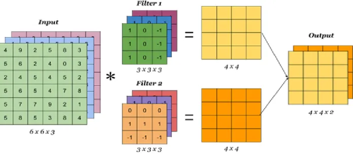
20 | P a g e Figure 6: An example of 2D convolutions. [24]

CNNs form the foundation of advanced computer vision methodologies. A convolution layer in a CNN is typically followed by a pooling layer. As shown in the Figure 7, high-level and low-high-level features are extracted from the image by passing it through multiple convolution and pooling layers. Finally, the obtained low dimensional feature vector is passed through a fully connected layer for inference and analysis.

Figure 7: A typical CNN architecture consisting of multiple consecutive layers of convolution and max pooling operations. [25]

(22)

21 | P a g e When the input image is convolved with the convolution kernel it loses the edge pixel values resulting with the input image being "trimmed" at the edges. This is because the pixels on the edge will never be located in the center of the convolution kernel, and the convolution kernel cannot be extended beyond the edge region. To solve this problem, a padding operation is often performed on the original image before performing the convolution operation. Padding involves filling zero values on the boundary of the image to increase the size of the image. With the padded image input, when the convolution kernel scans the input data, it can extend to the pseudo pixels beyond the edge, so that the output and input size are the same.

2.4.2

ResNet

The depth of the network is critical to the performance of the model. When the number of CNN layers in a network are increased, the network can extract more complex feature patterns, so theoretically better results can be obtained when the model is deeper. But experiments have found that in deep networks when the network depth increases, the network accuracy becomes saturated, or even decreases. This is because of the phenomenon called exploding or vanishing gradients. When the gradient is backpropagated from deeper layers, it becomes infinitively small due to repeated multiplication operation. Residual Network or ResNet [26] solves these problems by implementing skip connections between the output of the previous layers and the layer which is deeper into the network. ResNet was proposed by Kaiming He et al. [26].

(23)

22 | P a g e Figure 9: Overview of VGG19 architecture (left) and ResNet34 architecture

(24)

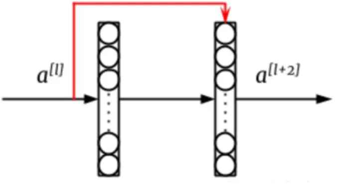
23 | P a g e Figure 8 shows the overview of the skip connections in deep neural networks. The red arrow depicts the skip connection. The activation 𝑎𝑙+2 is calculated as:

𝑧𝑙+2 = 𝑊𝑙+2 𝑎𝑙+1 + 𝑏𝑙+2 (4)

𝑎𝑙+2 = 𝑔𝑙+2 (𝑧𝑙+2 + 𝑎𝑙) (5)

where l represents the layer number, W represents the filter weight matrix, and a represents the data.

Table 1. Sizes of output and convolutional kernels for different variants of ResNet [26].

The structure of the ResNet network is similar to VGG19 [27] network with the addition of residual blocks and a greater number of layers. Figure 9 shows the structure of ResNet34 along with VGG19. Unlike VGG19, ResNet directly uses the convolution of stride = 2 for downsampling and replaces the fully connected layer with the global average pooling layer. Another important design principle of ResNet is that when the size of the feature map is reduced by half, the number of feature maps is doubled, which maintains the complexity of the network layer. As can be seen from Figure 9, ResNet adds skip-connections between every two layers compared to the ordinary network, which forms residual learning, where the dotted line indicates that the number of feature maps has changed. ResNet18, ResNet50, ResNet101 and ResNet152 are different variants of ResNet. As can be seen

(25)

24 | P a g e from the Table 1, for ResNet of 18-layer and 34-layer, the residual learning between the two layers is performed. When the network is deeper, the residual learning between the three layers is performed, and the three-layer convolution is performed. The kernels are 1×1, 3×3, and 1×1. Also, the number of feature maps of the hidden layer is relatively small, and it is 1/4 of the number of output feature maps.

Figure 10: Different residual blocks [26].

ResNet uses two different residual blocks, as shown in Figure 10. The left picture corresponds to the shallow network, and the right picture corresponds to the deep network. For skip-connections, when the input and output dimensions are the same, the input is directly added to the output. But when the dimensions are inconsistent, either zero-padding or 1×1 convolutions are used to increase the dimension.

2.4.3

PointNet

PointNet [2] introduced by Qi et al. is one of the pioneering works in the line of deep learning-based architectures for processing raw pointcloud data. PointNet [2] takes a raw pointcloud P without the need for any discretization or image-view projections and generates both a local feature vector encoding for each point and a global feature vector encoding representing entire pointcloud P. The authors demonstrate the effectiveness of the PointNet encoder in encoding the pointcloud data for the tasks of segmentation and classification of objects. Figure 11 shows the overview of the PointNet architecture. As shown in the top branch of Figure 11, the PointNet network takes a pointcloud P with n

(26)

25 | P a g e number of points as input and outputs classification scores for k classes. The bottom branch performs segmentation and outputs point-wise classification scores for m classes.

Figure 11: Overview of the PointNet architecture [2].

The input pointcloud is first passed through a spatial transformation network called T-net to generate an affine transformation matrix. A shared Multi-layer perceptron (MLP) with ReLU activation and batch normalization is then used to extract point-wise features from the input. The affine transformation matrix is used to align the features from different pointcloud data so that the model is invariant to feature space variance from different pointclouds. Note that both the T-net and MLP operations operate on one point independent of all others making the operation agnostic to point ordering. After two spatial transformation networks and two MLPs, 1024-dimensional features are extracted for each point. The point-wise features are aggregated together using a max pooling operation to create a global feature of size 1×1024 representing the whole pointcloud. Finally, the global feature vector is passed through a fully connected network to predict classifications scores for k predefined classes as shown in the top branch of Figure 11. Similar to the T-net and MLP operations, the global max pooling operation is also invariant to the order of the input points. In isolation, the global feature can be used for classification tasks. For tasks which need local structure information like part segmentation, local and global feature vectors are concatenated together resulting into a vector is size (n × 1088). This allows the prediction of the point-wise classification score for m predefined classes while considering both local and global information at the same time. The bottom branch of the Figure 11 performs point-wise segmentation.

(27)

26 | P a g e

2.4.4

VoxelNet

VoxelNet [9] is an extension and improvement over the PointNet [2] object detection network. VoxelNet [9] divides the space in fixed sized voxels and uses PointNet [2] on each voxel to encode information of the points in each voxel. This eliminates the need for hand crafted feature encoding on points in each grid.

Figure 12: Overview of the VoxelNet [9].

As shown in the Figure 12, voxel-wise features are extracted by passing each non-empty voxel through several Voxel Feature Encoding (VFE) layers. Each VFE is essentially a small PointNet [2] where first the point-wise feature vectors for all the points in a voxel are generated and then max pooling is applied to get locally aggregated voxel-wise features. This is followed by concatenation of point-wise and voxel-wise features to form a fixed size combined feature vector. The obtained fixed size feature vectors are consolidated as per their voxel-index and a sparse 4D tensor is generated. The 4D tensor is then fed through a stack of 3D convolutional layers resulting into a 3D feature map, which is then fed as input to a region proposal network (RPN) to perform 3DOD. The proposed

(28)

27 | P a g e RPN fuses high-level and low-level features by using a multi-scale feature aggregation technique.

2.4.5

Two Stage Network vs Single Stage Network

Deep learning-based object detectors can be categorized into two categories, namely two-stage detectors and single-two-stage detectors.

In the two-stage approach, first several class-agnostic region proposals are extracted from the image using a lightweight region proposal network (RPN), and then each of the candidate region proposals are passed through a classification network for object class detection and a bounding box regression network for localization. The main goal of the region proposal stage is to generate a finite number of region proposals for evaluation. Without a RPN, the potential bounding box candidates can be very large. Some of the pioneering work includes Fast CNN [16], Faster CNN [17], OverFeat [29], and R-FCN [30]. [29] uses sliding window approach for obtaining ROIs (Region of Interests) while [16] uses selective search. These are then passed into a region-based CNN to extract features for classification. Faster R-CNN [17] adopts a Region Proposal Network (RPN) which consists of a fully connected network to obtain ROIs.

In the single stage approach, the region proposal stage is skipped. The obtained feature maps corresponding to the dense sampling of possible locations are directly fed into a single stage unified CNN to predict class and bounding box coordinates. YOLOv3 [31], and MultiBox [32] are some of the examples of single stage detectors. In general, single stage detectors are faster than two stage but there is a tradeoff in accuracy.

2.5

Learning Loss Functions

Deep learning algorithms are data driven algorithms which require learning from numerous amounts of sample ground truth data. During the training stage, appropriate loss functions are used to calculate difference between the current network output and the desired ground truth. The task of the optimizer is to update the weights such as to minimize the loss. In the

(29)

28 | P a g e context of 3D object detection task, loss is comprised of two parts, the classification loss for object category distinction and the localization loss for bounding box offset prediction. The model loss is weighted sum of localization loss (SmoothL1) [16], and classification confidence loss (Focal loss) [33].

2.5.1

Focal Loss for Classification

Although the current single stage object detection algorithms, such as SSD [32] and YOLOv3 [31], achieve real-time speed, the accuracy cannot always be compared with the two stage Faster RCNN [17] object detection networks. A single-stage object detector usually produces up to 100k of candidate targets, and only a few of them are positive samples, with a large number of background targets. This leads to an imbalance of the sample ratio where too many negative samples during training lead to loss being too large and overwhelming the loss of positive samples. Lin et al. [33] proposed a new loss function called Focal Loss to address these issues and demonstrated significant improvement in the accuracies of single stage object detection networks. (6) shows the mathematical formula of Focal Loss.

𝐿𝑐𝑙𝑠 = {

−(1 − 𝛼𝑎) × (𝑝𝑎)Υ× log (1 − 𝑝𝑎) 𝑖𝑓 𝑦 = 0 −𝛼𝑎(1 − 𝑝𝑎)Υ× log(𝑝𝑎) 𝑖𝑓 𝑦 = 1

(6)

where 𝑝_𝑎 is the class probability of an anchor, y = 1 represents negative sample and y = 0 represents positive sample, and α, γ are hyperparameters.

The terms (1 - α) and α in (6) helps balance the imbalance between the number of positive and negative samples by reducing the loss due to negative samples in comparison to the loss from positive samples.

(30)

29 | P a g e Figure 13: Effect of different γ value on focal loss. [33]

Further, there is typically an imbalance between the number of easy-to-separate samples also called as easy-negatives and difficult-to-separate samples also called as hard-negatives. The easy-to-separate samples, that is, the samples with high confidence have very little improvement effect on the model, and the model should mainly focus on those difficult-to-separate samples. The loss due to the easy-to-separate samples is very low, but because the number of easy-negative samples versus the number of hard-negative samples is extremely high, the easy negative sample loss still dominates the total loss. The term

(1 − 𝑝𝑎)𝛾 𝑎𝑛𝑑 𝑝𝑎 𝛾

solves this imbalance between number of easy-negatives and number of hard-negatives by down-weighting easy samples and focus training on hard samples. For Example, γ when taken 2, if 𝑝 = 0.968, then (1 − 0.968)2 _{≈ 0.001}_{, resulting into}

1000-fold attenuation in the loss. In this way, the focal loss enables us to focus on hard positives, hard negatives, easy positives, and easy negatives in the order from high to low respectively during training phase. Experiments show that the best results are obtained when γ is taken as 2 as shown in Figure 13, and α as 0.25.

(31)

30 | P a g e Focal loss results in better accuracies in single stage detection and on par with the two stage detectors. This thesis uses focal loss function for classification.

2.5.2

Smooth L1 Loss for Bounding Box Regression

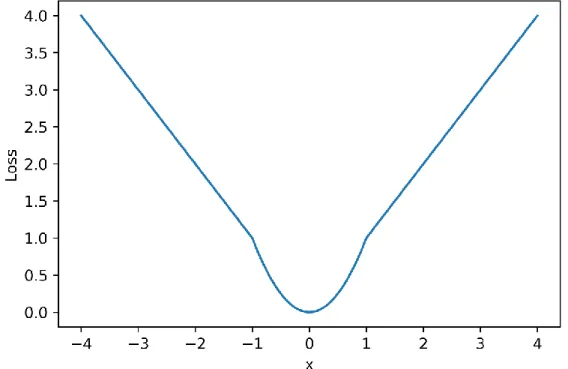
SmoothL1 loss is used for bounding box regression in most of the object detection networks like Fast RCNN [16], Faster RCNN [17], SSD [32], and many others. It is observed that SmoothL1 loss is less sensitive to outliers than L2. As shown in Figure 14, smooth L1 loss grows linearly with error rather than squarely. The difference between smooth L1 and L1-loss function is that the derivative of L1-loss at 0 is not unique, which may affect convergence. Hence, smooth L1 uses the square function around 0 to make it smoother as shown in (7).

Figure 14: Plot of smoothL1 loss.

𝐿_𝑙𝑜𝑐 = 𝐿_{1:𝑠𝑚𝑜𝑜𝑡ℎ} = { |𝑥| 𝑖𝑓 |𝑥| > 𝛼; 1

|𝛼| 𝑥

2_{𝑖𝑓 |𝑥| ≤ 𝛼}

(7)

(32)

31 | P a g e Combining (6) and (7), the total loss for the network is as follows:

𝐿 = 1

𝑁𝑝𝑜𝑠 (𝛽𝑙𝑜𝑐𝐿𝑙𝑜𝑐+ 𝛽𝑐𝑙𝑠𝐿𝑐𝑙𝑠)

(8)

where 𝛽_𝑙𝑜𝑐 = 2 and 𝛽_𝑐𝑙𝑠 = 1 are hyperparameters to weigh the localization and classification loss respectively. 𝑁𝑝𝑜𝑠 is the number of positive anchors.

2.6

Related Work

Accurate and Robust object detection has been extremely popular topic of research in mobile robotics and computer vision. Over the last decade, there have been significant advances in research and development of object detection methods using camera and LiDAR fusion. Most 3D object detection methodologies rely on cutting-edge 2D object detectors [7, 8, 10, 11, 12, 13, 14, 15]. In general, object detectors can be categorized into two categories, namely single-stage object detectors and two-stage object detectors. Further, depending on the type of data used by the detector, it can be grouped as image-based detector, pointcloud-image-based detector, and dual-modality image-based detector.

Mono3D++ [19] is a two-stage image-based detector. The first stage leverages the semantic information from the image and location priors to generate 3D object proposals at three different aspect ratios. The second stage utilizes the generated object proposals to regress 3D bounding box coordinates. [15], [20] are similar two-stage image-based detectors that generate priors by utilizing only RGB images and then estimate 3D bounding boxes. The inference time of these networks is around 0.7 seconds per sample proving to be inadequate for real-time applications.

[2, 3, 14, 21] are some of the examples of pointcloud-based object detectors where, first the pointcloud is divided based on nearest neighbor clustering and then features are extracted from those clusters using 3D CNNs. The process of clustering a pointcloud is computationally expensive and time consuming unlike voxelizing the pointcloud into

(33)

32 | P a g e multiple regular voxels as proposed by VoxelNet [9]. Pointpillar object detector [7] is another example of single-stage pointcloud-based detector.

Eduardo et al. [8] provides an in-depth overview of 3D object detection methods and discusses various available datasets for 3DOD. The paper highlights the advantages and disadvantages of fusion based methods in contrast with LiDAR-only and camera-only methods.

PointNet [13] and RoarNet [22] are examples of two-stage dual-modality based detectors. They leverage the data from LiDAR and camera in sequential fashion. Frustum PointNet [13] generates 2D region of interests (RoIs) proposals from the RGB camera image which are then projected onto the 3D LiDAR pointcloud data to obtain 3D frustum proposals. The obtained frustum proposals are then passed through a PointNet [2] for bounding box regression.

VoxelNet [9] uses only LiDAR pointcloud data to perform 3DOD. First the point cloud is discretized into multiple evenly spaced voxels, following which local features are extracted from each of these voxels using PointNet. These features are then consolidated into a 4D tensor and passed through a 3D CNN to further extract features for final classification and regression of 3D bounding boxes. Due to the expensive 3D convolution operation, the inference speed of VoxelNet is about 4.44 Hz.

AVOD [23] and MV3D by Chen et al. [11] are examples of late fusion of LiDAR and camera data to perform 3DOD. In AVOD [23], the point cloud data is projected onto the XY plane to obtain a BEV image of the vehicle’s surrounding. This allows for a faster and light weight single modality CNN based network, while sacrificing 3D geometrical information such as height for each point in the point cloud.

MV3D [11] transforms the pointcloud data into image modality by projecting the points in the pointcloud onto XY plane and YZ plane to obtain BEV and front view (FV) projection images. Height, intensity and density information is obtained from the points in the point cloud and encoded into the BEV projection, while height, distance and intensity

(34)

33 | P a g e information with respect to front view are encoded into the FV projection maps. The region proposal network uses BEV projection images to generate RoI proposals. FV images and RGB images are encoded using separate CNN based encoders and the obtained feature representations are fused together by a deep fusion network. The inference speed is about 2.7Hz. Despite good performance on the KITTI benchmark dataset [18] for car detection, these methods are not efficient for detecting smaller objects like pedestrians.

F-PC-CNN [12] performs early fusion of LiDAR-camera data to estimate 3DOD parameters. A region proposals network generates 2D RoI proposals from RGB images. A subset of points from the pointcloud which spatially align with the obtained 2D proposals are selected and a deep CNN network is used to obtain oriented 3D bounding boxes.

(35)

34 | P a g e

Chapter 3

Methodology

3.1

Pointpillar Encoder – Baseline

Pointpillar [7] is a pointcloud encoder which uses PointNet [2] to extract global as well as local spatially invariant features from the pointcloud. The input 3D pointcloud is converted into a 2D pseudo Bird’s Eye View (BEV) projection image-like vector constructed by extracting learned features across the Z axis of the pointcloud. The inventors of the Pointpillar encoder use a lean downstream object classification network to demonstrate the efficiency and effectiveness of the encoder for the task of 3DOD with only LiDAR pointcloud data as input. The resulting network is an end-to-end learnable network with real-time inference of 16ms per pointcloud sample.

Figure 15: Overview of the Pointpillar architecture [7], D = Number of point features (9), P = Maximum number of pillars per sample (12000), N = Number of points per pillar (100) C = Number of pseudo-image feature maps (64), H,W = Height and Width of the feature maps (496 × 432).

(36)

35 | P a g e The architecture of the Pointpillar 3D object detector is very similar to VoxelNet [9] 3D object detector comprising of three main components, namely, Pillar Feature Net (PFN), Middle Feature Extractor (MFE) and a downstream classification network. Figure 15 shows the architecture overview of the Pointpillar 3D object detector. First, a BEV of the pointcloud is discretized into evenly spaced grid in the X-Y plane by bounding the point cloud into multiple vertical columns also known as pillars.

Discretization of the pointcloud generates a tensor of shape (D × P × N). The discretized BEV X-Y plane grid of bins would mostly contain empty pillars. This sparse nature is true even for high-resolution LiDARs. While P could represent each of these X-Y locations, it is more efficient for P to be a vector containing only the non-empty pillars. Each of these non-empty pillars has up to N points. Each of these N points has D features as shown in (9).

𝑙 = [𝑥, 𝑦, 𝑧, 𝑟, 𝑋_𝐶, 𝑌_𝐶, 𝑍_𝐶, 𝑋_𝑃, 𝑌_𝑃] (9)

where x,y,z represent the XYZ cartesian coordinate of the point l, 𝑟 is the reflectance value,

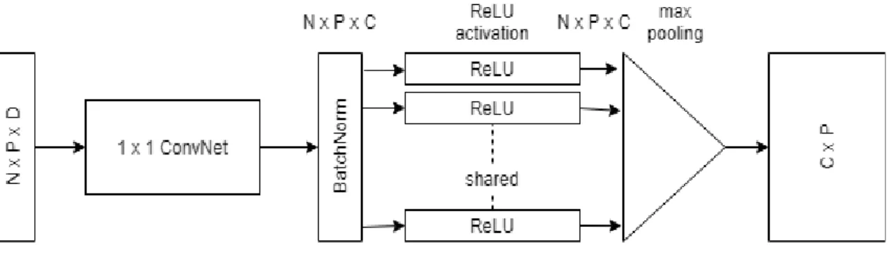
𝑋_𝐶, 𝑌_𝐶, 𝑍_𝐶 are offset from the arithmetic mean of all the points in the pillar, and 𝑋_𝑃, 𝑌_𝑃 are the 𝑥 and 𝑦 offset from the pillar center. If P, the maximum number of non-empty pillars, or N, the maximum number of points per pillar exceeds the tensor size, points are randomly sampled to reduce computational complexity. If a pillar has fewer points, zero padding is applied. This yields a dense tensor of shape (D × P × N). The PFN layer consists of a simplified PointNet layer where each point of the pointcloud is processed by three operations, a linear operation, followed by batchnorm and finally a ReLU activation yielding a tensor of shape (C × P × N) as shown in Figure 16. Further, a pillar-wise max pooling operation is performed, to extract features across the vertical columns resulting in a vector of shape (C × P) where C is the number of feature maps to be generated for pseudo-image features. The features obtained are based on the learned weights of the PFN thus eliminating the need for handmade features and making the network end-to-end learnable. The obtained features are then consolidated according to their pillar index and transformed into a pseudo image-like BEV 2D feature maps of size H × W, yielding a C × H × W

(37)

36 | P a g e shaped tensor which is then passed through a 2D CNN backbone network to extract further high level features.

Figure 16: Simplified PointNet Architecture.

The 2D CNN backbone network has two sub-networks. The first network is a top-down network like the one in Multi-Box detector [32] comprising of series of 2D convolutions and deconvolution layers which generate features from the input pseudo-images at different resolutions. The second network upsamples and concatenates the top-down features which are then fed to a 3D SSD network to predict the object classes and regress 3D bounding boxes.

The main difference in Pointpillar architecture and VoxelNet [9] architecture is in way in which they extract local and global features and how they perform global pooling on local features. The Pointpillar object detector is based on an assumption that in a typical outdoor road scenario no two objects are on top of each other and hence unlike VoxelNet it constructs voxels with larger height (pillars) covering the whole frame of interest in the ZY plane. This indeed allows the middle feature extractor to consolidate the feature vectors obtained from PFN by performing a single global pooling based on the pillar index to obtain a 2D image like vector. This eliminates the need for a 3D convolution network to further extract high level features in the Middle Feature extraction stage. Finally, they use multi-box single shot detector as a downstream classification network to predict object classes in the scene and regress their 3D bounding box coordinates. Apart from state-of-the-art inference speed of about 60Hz, the Pointpillar 3D object detector significantly

(38)

37 | P a g e outperforms all the other LiDAR-only networks on KITTI 3D object detection benchmarks [18].

3.2

Proposed Architecture

A multi-modal approach is needed to build a robust and accurate 3D object detector. A model built by a multi-modal approach can be significantly better in representing the surrounding and capturing the variability. Deep learning-based encoders are data driven. Data from multiple sources can provide more unique information and more variant data. The vector representation obtained from such a model can have applications in other 3D perception-based tasks such as path planning, machine-world interaction, augmented/virtual reality which are essential part of the autonomy stack of many intelligent systems. Multi-modal fusion is a relatively new field of research and has its own challenges. Some of the challenges include real-time inference, relatively larger model size compared to single sensor detection networks, highly distant feature vector space of the vector representations obtained from individual modality encoders, training strategies, coherent and synchronized dataset generation, and many more.

An efficient fusion strategy is needed to address these issues and exploit information from multiple sensor sources. LiDAR and camera together provide adequate enough information needed for 3DOD tasks, as camera provides us with rich texture information in terms of incident light, and LiDAR provides us with relative depth information of the objects around the machine and their 3D geometrical shape.

The Pointpillar 3D object detector is chosen as the baseline architecture and is modified to enable multi-modal data input. The goal of the Pillar Feature net (PFN) is to reduce the dimensionality of the input voxelated data, keeping only the useful features and removing the features that would be redundant or slow down or confuse the model. Discarding the Z dimension and projecting the point cloud on the XY plane gives us a bird’s-eye view of the vehicle surroundings. MV3D and other literature hardcoded the handcrafted features. Instead, PFN enables us to let the neural network learn which features to keep and which to discard. Additionally, the setup of PFN enables augmentation of point features of the

(39)

38 | P a g e point cloud with n number of other features from a variety of other sensor data like RADAR, cameras, secondary LiDARs, etc. The main advantage of choosing Pointpillar object detector is its real-time performance and its three-stage architecture which enables implementation of different fusion strategies with fewer amendments.

We discuss the three fusion strategies, namely, early fusion, late fusion and combined fusion in the following sections. All the fusion model encodes the pointcloud data into pseudo image-like vector, using Pointpillar [7].

3.2.1

Early Fusion

Early fusion in deep networks is defined as a fusion strategy where the data is fused together with or without preprocessing of the individual modality before feeding into any neural network pipeline. Figure 17 shows the overview of the early fusion architecture for 3DOD task using LiDAR pointcloud and camera image data. The first stage of the Pointpillar object detector is the Pillar Feature Net (PFN). PFN is tasked with extracting learned features from the pointcloud across the Z axis and convert it into a pseudo image-like vector. The augmented pointcloud point l has D = 9 features in the original Pointpillar network,

𝑙 = [𝑥, 𝑦, 𝑧, 𝑟, 𝑋_𝐶, 𝑌_𝐶, 𝑍_𝐶, 𝑋_𝑃, 𝑌_𝑃] (9)

where 𝑋_𝑃 and 𝑌_𝑃 are the 𝑥 and 𝑦 offset from the pillar center, 𝑋_𝐶, 𝑌_𝐶, 𝑍_𝐶 are offset from the arithmetic mean of all the points in the pillar, and 𝑟 is the reflectance value from the LiDAR.

(40)

39 | P a g e Figure 17: Architecture overview of the proposed Early Fusion network.

The PFN layer is modified such that it takes a pointcloud augmented with the corresponding RGB values of the environment obtained from the camera image resulting into a point l with D = 12 features. The RGB value for a particular point is obtained by projecting the 3D point from the LiDAR frame of reference onto the image in the image frame of reference using the rotation and projection matrices provided by the KITTI development kit and then getting the RGB value for that particular point from the pixel location where the projected point overlaps with the image pixel.

A point 𝑥 = (𝑥, 𝑦, 𝑧, 1)𝑇 in LiDAR coordinate frame can be projected to a point 𝑦 = (𝑢, 𝑣, 1)𝑇_{in the}_𝑖𝑡ℎ_{camera image frame following the equation below,}

𝑦 = 𝑃_{𝑟𝑒𝑐𝑡} × 𝑅_{𝑟𝑒𝑐𝑡} × 𝑥 (10)

where 𝑃𝑟𝑒𝑐𝑡 and 𝑅𝑟𝑒𝑐𝑡 are the extrinsic rectified projection and rotation matrices,

respectively. The resulting augmented LiDAR point l with D =12 features as in (3) below is then fed into the modified Pointpillar network (Figure 3.3) to obtain 3DOD predictions.

(41)

40 | P a g e

𝑙 = [𝑥, 𝑦, 𝑧, 𝑟, 𝑋_𝐶, 𝑌_𝐶, 𝑍_𝐶, 𝑋_𝑃, 𝑌_𝑃, 𝑅, 𝐺, 𝐵] (11)

We perform an additional mean filter convolution operation for the input image obtained from the camera before overlaying the pointcloud on the image in order to normalize sensitivity to RGB pixel values, without which the convergence of the network was irregular and individual batch loss was very high. The mean filter takes the average of all the pixels that lie below it while convolving over the entire image and replaces the central pixel with the new average value. The filter kernel of size 5 × 5 was carefully chosen as it gave the best performance in terms of accuracy and mean average precision (mAP). Figure 18 shows example of a sample before and after mean filter operation.

Figure 18: Effect of Average filer. Original Image (Left), Mean Filtered Image (5×5 kernel)(Right)

3.2.2

Late Fusion

Late fusion in deep networks is defined as a fusion strategy in which the information from different data sources is fused after it has been encoded in lower dimensional vector representations using individual encoders for each data modality. After encoding the data in the encoder stage, a joint feature vector is constructed by combining the encoded feature vector of the individual modality. Late fusion is popular for fusion of data of various dimensions, such as image, pointcloud and analog data, as representations of vectors can easily be concatenated with each other in a learned network. Late fusion enables the application of specialized encoders for each modality type with independent processing of individual raw sensor data. This independence could theoretically lead to more accurate

(42)

41 | P a g e vector representations of the input data. This strategy automatically assigns weights to the inputs during the training phase, without any manual tuning required. Unlike the early fusion model, even if data from one of the two modalities is missing, late fusion will still be able to provide 3DOD.

Figure 19: Architecture overview of the proposed Late Fusion network.

Figure 20: ResNet like CNN architecture for image feature extraction.

Figure 19 shows the overview of the late fusion architecture. In our case, the two modalities are the pointcloud and the image which are encoded by their respective encoders. LiDAR pointcloud data is encoded using the Pointpillar encoder and camera image data is encoded using a ResNet-like architecture as discussed below. PointPillar encodes the pointcloud data into 64 image-like feature maps of size 496 × 432. The popular ResNet18 architecture

(43)

42 | P a g e is modified as shown in Figure 20 to encode image data and extract feature maps. The camera image data is resized to 3 × 224 × 224 before feeding into the modified ResNet18 architecture which extracts important features from the input image and generates 128 feature maps of size 28 × 28 each. These feature maps are then upscaled to 496 × 432 using bilinear interpolation to combine with the 64 feature maps obtained from the PointPillar encoder to form a unified joint vector representation of the data from the two input sensors. The fused feature maps are then passed to an SSD network where the 2D CNN backbone network discussed in Section 3.1, further extracts learned features from the fused representation at various resolutions. The weights of the filters in this 2D CNN backbone are learned during the end-to-end training of the whole network. Thus, these fused representations contain the synchronized information from both input modalities. Finally, the multi-resolution feature maps obtained from the backbone network are concatenated and an SSD head performs object classification and regression for 3D bounding box coordinates.

3.2.3

Combined Fusion

Figure 21: Architecture Overview of the Combined Fusion network, EF = Early Fusion, LF = Late Fusion.

(44)

43 | P a g e The two fusion models discussed in the section above capture the features from the input data at different levels. We propose a combined fusion model which incorporates both late fusion and early fusion in a sequential manner. Figure 21 shows the overview of combined fusion model. First, Early fusion is performed in the first branch, marked as "EF" and late fusion is performed after the encoder stage marked as "LF." The first branch consisting of the PFN encodes the RGB augmented point cloud data and generates 64 pseudo image-like feature maps. Features from the RGB image are extracted using the CNN architecture shown in figure 3.6. The feature maps from these two branches are concatenated using the late fusion model and then transferred though the 2D CNN backbone, followed by SSD head to obtain object classification scores and 3D bounding boxes.

(45)

44 | P a g e

Chapter 4

Implementation

4.1

KITTI 3D Object Detection Benchmark Dataset

All the evaluations are done using the KITTI object detection benchmark dataset [3], which is built by the Karlsruhe Institute of Technology in conjunction with Toyota Technological Institute at Chicago. The KITTI dataset [3] consists of six hours of real-world road traffic scenarios recorded at 10Hz-100Hz using a variety of sensors. It has about 200k 3D object annotations for image data from four HD cameras as well as corresponding point cloud data from a Velodyne LiDAR. The cameras, laser scanner and the localization system are all calibrated and synchronized. Each scene has up to 15 cars and 30 pedestrians. The data is split into 7,481 training samples and 7,581 testing samples. The ground truth labels for the test set are not publicly available. Evaluation on test data can be obtained by submitting the prediction results to the online benchmark server. Hence, we follow the training set split provided by the MV3D [11] which is commonly used by many other similar works. The training set is split into a new training set of 3712 samples and a validation set of 3769 samples. Depending on the number of truncations and occlusion in the scene, each annotation label is marked as either ‘fully visible’, ‘partly occluded’ or ‘largely occluded’ target. The annotations are further divided into three groups considering the detection difficulty for that particular annotation.

Table 2. Thresholds for difficulty levels of the annotations [3].

Difficulty min. bounding box height

max. occlusion level max. truncation Easy 40 pixels Fully visible 15 % Moderate 25 pixels Partly occluded 30 % Hard 25 pixels Largely occluded 50 %

(46)

45 | P a g e Figure 22: Sensor placement scheme of the car used to collect KITTI dataset [3].

We use the LiDAR scans and left front RGB camera images. An example from the dataset is shown in Figure 23. Annotations are provided in the form of 3D Bounding Box tracklets in the camera frame of reference. Seven classes are defined, namely ’Car’, ’Truck’, ’Person (sitting)’, ’Pedestrian’, ’Tram’, ’Cyclist’, and ’Misc’. Each object has an associated class, 3D bounding box and yaw angle in every frame. Car, Pedestrian, and Cyclist are the three dominant classes in the dataset, hence the 3D object detection challenge requires to report metrics and scores for these three classes only. There are few instances where the object classes are present in the camera image but are not visible in the corresponding point cloud because of the increase in the sparsity of points with distance. Such object cases are labelled as ‘DontCare’ to prevent false positives during evaluation.

(47)

46 | P a g e Figure 23: An example from the KITTI dataset.

4.2

Evaluation Metrics

Average Precision (AP) and Intersection over Union (IoU) are commonly used for performance evaluation of object detectors. The IoU score is defined as the ratio between the area of overlap and the area of union, where area of overlap is the area of intersection between the predicted and the ground truth bounding box, and area of union is the area encompassed by both, the predicted bounding box and the ground truth. Figure 24 shows the depiction of IoU.

KITTI [18] defines a predicted box as true positive (TP), if its IoU score exceeds the threshold of 0.7 for “Car” category and 0.5 for “Pedestrian” and “Cyclist” category. Similarly, a predicted box is considered false positive (FP) if its IoU score is less than the threshold. A false negative (FN) is defined when the network does not detect a real object present in the scene.

𝐼𝑜𝑈 = 𝐴𝑟𝑒𝑎 𝑜𝑓 𝑜𝑣𝑒𝑟𝑙𝑎𝑝 𝐴𝑟𝑒𝑎 𝑜𝑓 𝑢𝑛𝑖𝑜𝑛

(48)

47 | P a g e Figure 24: Visualization of Intersection over Union.

As in (13), precision is defined as the ratio of the number of detected TPs to the total number of detections. Precision basically measures what percentage of the model predictions are correct.

Recall represents how efficient the model is at detecting the true positives. It is defined as the ratio between total number of TPs and total number of ground truths as shown in (14).

The KITTI Benchmark [18] defines average precision (AP) as the average of the precision values at each of eleven predefined recall values. The maximum precision value is taken to calculate the mean. Equation (15) shows how AP is calculated.

Precision = 𝑇𝑟𝑢𝑒 𝑃𝑜𝑠𝑖𝑡𝑖𝑣𝑒 𝑇𝑟𝑢𝑒 𝑃𝑜𝑠𝑖𝑡𝑖𝑣𝑒 + 𝐹𝑎𝑙𝑠𝑒 𝑃𝑜𝑠𝑖𝑡𝑖𝑣𝑒 (13) Recall = 𝑇𝑟𝑢𝑒 𝑃𝑜𝑠𝑖𝑡𝑖𝑣𝑒 𝑇𝑟𝑢𝑒 𝑃𝑜𝑠𝑖𝑡𝑖𝑣𝑒 + 𝐹𝑎𝑙𝑠𝑒 𝑁𝑒𝑔𝑎𝑡𝑖𝑣𝑒 (14) AP = 1 11 ∑ max [𝑝 ( 𝑟 10)] 10 𝑟=0 (15)

(49)

48 | P a g e

4.3

Implementation

All the three fusion networks as well as the baseline network are trained in an end-to-end manner. We follow the same training strategy as in the original Pointpillars paper [7], which involves matching strategy for default bounding box selection for each ground truth bounding box, hard negative mining, and choosing aspect ratio and scales for default anchor boxes.

Matching strategy involves finding the correct anchor boxes which match the ground truth targets. Each anchor box contains aspect ratio, scale, and location. A class anchor is defined by height, length, width and z center. Anchors and ground truth are matched using 2D IoU. A match is considered positive if the IoU is above the set positive match threshold. Similarly, a match is negative when the IoU is below the negative threshold. Only the matched anchors contribute towards the loss. This simplifies the learning problem and allows the network to predict high scores for multiple overlapping anchor boxes. During inference, anchors are filtered out using non maximum suppression (NMS) with overlap threshold values of 0.5 IoU.

An object classifier needs to be trained on both foreground samples (objects of interest) also referred as positive samples as well as background samples also referred as negative samples) so that it learns to distinguish between what constitutes as foreground and background. Generally, any real-world scene will have fewer foreground samples compared to background samples. Hard negative mining is performed in order to prevent imbalances between the number of positive samples and number of negative samples. During training, Top K negative samples are selected based on their objectiveness score to contribute towards the network’s loss. K for each batch is calculated to maintain a ratio of 1:3 foreground to background samples for each batch.

As the network parameters vary greatly with the size of the object being detected, two separate networks are trained. One for detection of “Cars”, and other for “Pedestrians and Cyclists”. The implementation and training of the network is done using the Pytorch

(50)

49 | P a g e framework. Table 2 shows the configuration setup for the baseline as well as the fusion models. All the weights are initialized with uniform random distributions. All the three fusion models and the baseline model are trained for 220 epochs with batch size of 2 on the training set of the KITTI dataset [3]. The initial learning rate is set as 0.002 with a decay factor of 0.8 every 15 epochs. The loss functions discussed in Section 2.5 are employed and optimized using the Adam optimizer during training.

Table 3. Configuration setup for Baseline, Early fusion, Late Fusion and Combined Fusion model.

Car Network Cyclist-Pedestrian Network

Point cloud range ([xmin, xmax] × [ymin, ymax] ×

[zmin, zmax]) [0, 69.12] × [-39.68, 39.68] × [-3, 1] [0, 47.36] × 19.84, 19.84] × [-2.5, 0.5] Voxel size [0.16, 0.16, 4] [0.16, 0.16, 3] Max number of pillars (P) 12000 12000 Max number of points per pillar (N) 100 100

Classification loss weightage 1.0 1.0 Localization loss weightage 2.0 2.0 Default anchor box sizes (w, l, h):

[1.6, 3.9, 1.56]

Car : [1.6, 3.9, 1.56] Cyclist : [0.6, 1.76, 1.73] Pedestrian: [0.6, 0.8, 1.73] Positive matching threshold 0.6 0.5

(51)

50 | P a g e

Chapter 5

Results and Analysis

5.1

Results

“Car”, “Pedestrian” and “Cyclist” are the three dominant classes out of the seven classes in KITTI dataset [3]. We train and evaluate our models on these three classes. The models are evaluated for the task of BEV and 3D object detection based on IoU and mAP scores as defined by the KITTI evaluation metrics [18]. Depending on the truncations and occlusions of the annotation, each annotation is categorized based on the difficulty level of detection as either “Easy”, “Moderate” or “Hard”. Table 4 shows the results for 3D object detection task and Table 5 shows the results for BEV detection task.

Table 4. 3D detection benchmark scores

Results on KITTI val (3769 examples), trained on KITTI train (3712 examples)

Method

mAP (Mo

d)

Car (IOU = 0.7) Pedestrian (IOU = 0.5) Cyclist (IOU = 0.5) Easy Mod. Hard Easy Mod. Hard Easy Mod. Hard Baseline 58.03 81.49 67.89 65.99 60.80 56.31 50.42 70.18 50.04 47.07 Early Fusion 60.30 84.15 70.34 66.12 62.79 58.42 51.22 72.43 52.16 47.83 Late Fusion 57.20 81.23 66.42 63.11 59.84 56.33 50.12 69.13 48.86 46.02 Combin ed Fusion 60.44 84.67 70.84 64.88 63.14 58.13 51.88 72.44 52.34 47.17

(52)