Maximum likelihood estimation for stochastic processes - a martingale approach

A M A R T I N G A L E A P P R O A C H

by

Paul David F ei gi n

Thesis submitted for the degree of Doctor of Philosophy of the Australian National University

A C K N O W L E D G E M E N T S

I wish to express my sincere gratitude to Professor C.R. Heathcote and to Dr C.C. Heyde, both of whom have supervised my work over the past two and a half years. I am especially grateful to Dr Heyde for the suggestions that stimulated the bulk of the research reported here, and for his conscientious and constructive criticisms. I am also indebted to Professor E.J. Hannan for his advice and discussions on several issues that arose in the course of this research. Among the many other teachers, colleagues and friends who have contributed to my understanding of various areas of probability and statistics, I wish to mention particularly Dr R.L. Tweedie and Dr E. Seneta.

I am also grateful for having had the opportunity to study at the Australian National University. To all the staff of the Statistics Departments, and especially to Professor R.D. Terrell, I wish to express thanks for providing me with the opportunities that made working and teaching here a satisfying and rewarding experience.

I would also like to express thanks to Mrs H. Patrikka for typing drafts of parts of the thesis as well as to Mrs B. Geary for her excellent typing of the final manuscript.

ABSTRACT

This thesis is primarily concerned with the investigation of asymptotic properties of the maximum likelihood estimate (MLE) of parameters of a

stochastic process. These asymptotic properties are related to martingale limit theory by recognizing the (known) fact that, under certain regularity conditions, the derivative of the logarithm of the likelihood function is a martingale. To this end, part of the thesis is devoted to using or

developing martingale limit theory to provide conditions for the consistency and/or asymptotic normality of the MLE. Thus, Chapter 1 is concerned with the martingale limit theory, while the remaining chapters look at its

application to three broad types of stochastic processes. Chapter 2 extends the classical development of asymptotic theory of MLE’s (a la Cramer [1]) to stochastic processes which, basically, behave in a non-explosive way and for which non-random norming sequences can be used. In this chapter we also introduce a generalization of Fisher's measure of information to the

stochastic process situation. Chapter 3 deals with the theory for general processes and develops the notion of "conditional" exponential families of processes, as well as establishing the importance of using random norming sequences. In Chapter 4 we consider the asymptotic theory of maximum

likelihood estimation for continuous time processes and establish results which are analogous to those for discrete time processes. In each of these

chapters many applications are considered in an attempt to show how known and new results fit into the general framework of estimation for stochastic processes.

TABLE OF CONTENTS

ACKNOWLEDGEMENTS (ii)

ABSTRACT (iii)

CHAPTER 0. INTRODUCTION

0.§1 The Thesis in Perspective 1

0. §2 Notation 5

CHAPTER 1. MARTINGALE LIMIT THEORY

1. §1 Motivation and Rationale 9

l.§2 Analogues of the Laws of Large Numbers 11

l.§3 Central Limit Theorems 15

l.§4 Vector Martingales 23

1. §5 Continuous Parameter Martingales 33

CHAPTER 2. ML ESTIMATION - NON-RANDOM NORMING THEORY

2. §1 The Statistical Framework 51

2.§2 Consistency of the MLE 54

2.§3 Asymptotic Normality of the MLE 64

2.§4 Applications 70

2. §5 Comparisons with Previous Results 92 CHAPTER 3. ML ESTIMATION - RANDOM NORMING THEORY

3. §1 Motivation 105

3.§2 Conditional Exponential Families and Inference 108 3.§3 Consistency of the MLE in General 115

3.§4 Applications 118

3. §5 The Vector Parameter Case 144

CHAPTER 4. ML ESTIMATION - CONTINUOUS TIME PROCESSES

4. §1 The Likelihood Function 146

4.§2 The Martingale Theory 150

4.§3 Estimation for Diffusions 154

4.§4 Estimation for Pure Jump Processes 172

4.§5 An Illustrative Calculation 185

APPENDIX A. ML ESTIMATION FOR BRANCHING PROCESSES

A.§1 Non-Parametric Case 188

APPENDIX B. THE EMPIRICAL CHARACTERISTIC FUNCTION

B.§1 Motivation and Preliminaries 197

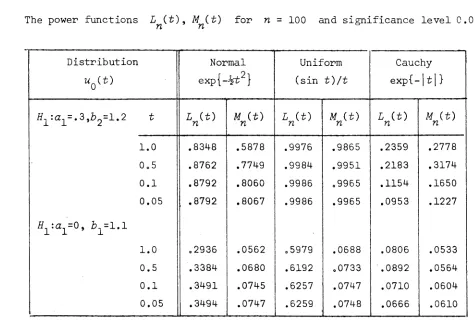
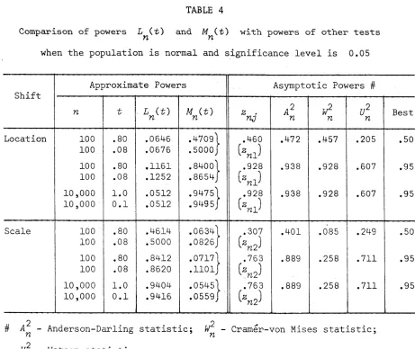
B.§2 Goodness of Fit Tests 202

B.§3 Relationship with the Cramer-von Mises Statistic 209

C H A P T E R 0

I N T R O D U C T I O N

§1. T he T he si s in P e r s p e c t i v e

This work is primarily concerned with the asymptotic theory of maximum likelihood (ML) estimation for stochastic processes. The key to this

asymptotic theory is the recognition of the fact that (under regularity conditions) the derivative of the logarithm of the likelihood function is a martingale. In the classical problem, that of independent and identically distributed random variables ( i .i .d.r.v . ’s ), this martingale is just the sum of i.i.d.r.v.’s itself, and so is the subject of well known limit theorems. Because of the relationship between the derivative of the logarithm of the likelihood and the maximum likelihood estimate (MLE), we can often use these limit theorems to prove asymptotic properties of the MLE. This relationship holds also for the stochastic process situation, however, we now need limit theory for martingales to prove corresponding asymptotic theory for the MLE. This fact was probably first made explicit by Silvey [1], although only in the more limited context of Chapter 2 - the non-random norming situation.

Before we describe the martingale approach in more detail we will

briefly discuss other work on inference for stochastic processes. Actually, there have been very few attempts at a general theory (rather than solving particular problems) of inference for stochastic processes. One such

contribution was that of Grenander [1], whose work was largely concerned with continuous time processes. He suggested the reduction to ’’observable

the possible use of a random norming sequence. Grenander’s work also covers hypothesis testing, a topic that will not be covered in this work. (Having established the asymptotic theory for the MLE, it is often quite straight­ forward to compute the asymptotic properties of the likelihood ratio test

(see, for example, Billingsley [2]). This type of computation has not been made explicit here, but will be the subject of subsequent work.)

Some further significant work on inference for stochastic processes is included in Bartlett [1]. In a way, this thesis is an attempt to meet the "challenge" expressed in §8.11 of Bartlett’s book:

"The known theorems on the asymptotic theory of maximum-likelihood estimates do not in general apply to dependent observations 3 and have to be extended. These extensions . . . are associated with the extension of the Central Limit Theorem to dependent observations." Again, Bartlett’s work is largely concerned with stationary processes, and when he does consider the birth-death process he uses a stopping rule for

the estimation procedure (see 4.§1 for some discussion of this approach). In two papers, M.M. Rao [1, 2] discusses the asymptotic theory of ML estimation for stochastic processes. For the discrete time case, he extends the results of Wald [1] (see below) concerned with the consistency of the MLE of a scalar parameter. He does not completely extend his results to the vector case (as we do in Chapter 2) because his approach does not allow for a different norming for each component of the vector of derivatives of the logarithm of the likelihood. Rao [2] defines "wide sense efficiency" and consequently does not need to prove the asymptotic normality of the MLE’s to claim their efficiency. This approach avoids the need to use random

normings in many cases, although the result may be considered of little use in conducting inference based on the asymptotic distribution. In his work, Rao also does not make use of the martingale property mentioned earlier.

contiguity and does not use the martingale property.

Another contribution to ML estimation for dependent observations has been made in two papers by Weiss [1, 2], which are discussed in detail in 2.§5. These do not use the martingale property and are restricted to non-random norming sequences. There are also two related papers by Bar-Shalom [1], and Bhat [1], which only consider the classical norming, \fn . Both these papers contain errors discussed in 2.§5. An early paper by Wald [1] gives conditions under which the MLE for a stochastic process will be

consistent. These conditions are closely related to those of Chapter 2 but do not make use of the martingale theory. Wald also only considers non-random norming.

There have been many articles concerned with the asymptotic properties of MLE's for particular processes. In the examples and applications of the following chapters, these papers are referred to in context and so we will not pursue a discussion of them here.

All the above discussion has been concerned with ML estimation for stochastic processes. There has recently appeared a discussion of maximum probability estimators (Weiss and Wolfowitz [1]) which incorporates the stochastic process situation as well (at least for discrete time processes). The results seem to be quite general and, theoretically, may suggest the removal of the MLE from "centre-stage" in the theory of estimation. The main advantage of the MLE (in most cases) is that it is easily computed from

the likelihood equation. This advantage is, of course, of very great practical importance. Nevertheless, it may be valuable to investigate the

consequences of applying Weiss and Wolfowitz’s theory to some of the examples that follow. The fact that their theory does not use the martingale

We have, in several instances in the preceding discussion, mentioned the notions of random and non-random norming (or norming sequences). The introduction of random norming sequences is a consequence of the desire to prove laws of large numbers and central limit theorems (CLT’s) for

martingales. Part of the theme of Chapter 1 is the demonstration of the appropriateness of a particular random norming in the martingale context. This type of random norming opens the way to the required limit theory for martingales, which, in turn, provides the main tool in proving asymptotic properties of the MLE. Moreover, this particular random norming plays the role of Fisher’s measure of information in the stochastic process context

(see 2.§2 for some details), when considering the martingale which is the derivative of the logarithm of the likelihood. The ramifications of this generalization of the classical measure of information are explored in several places in the development of the thesis.

The first use of a random norming to prove an asymptotic normality

result for an estimator seems to have been by Anderson [1], although he makes no special point of this fact. More recently, in connection with estimation

for supercritical Galton-Watson processes (see 3.§4), several authors have used such random normings (see, for example, Heyde [5] and Dion [1,2]). Also, for the birth-death process, Keiding [1, 2] proves the asymptotic normality of the MLE’s of the birth and death parameters using random normings. Only Heyde [5] mentions the significance of the use of random norming sequences for stochastic process estimation, which is further discussed in Heyde and Feigin [l].

A simplified scalar version of some of the material of Chapter 2 (non-random norming) has appeared in a paper by Basawa, Feigin and Heyde [1],

between the two estimators and so we feel there is no serious abuse in referring to the former as "the" MLE.

Although the theory of the sequel is developed for stochastic processes in general, most of the illustrative applications are to Markov processes. This restriction comes from the difficulty of modelling, in a mathematical way, other types of dependence, and is particularly true for the continuous

time processes with the result that all the applications of Chapter 4 are to Markov processes.

The two appendices deal with areas that are not directly related to asymptotic theory of MLE’s. Appendix A provides some supplementary results on ML estimation for branching processes and discusses a conjecture of Speed [1]. Appendix B is a report of some work on inference for i.i.d.r.v.’s using the empirical characteristic function. This approach complements the major part of the work in that it provides an alternative to inference based on the likelihood and is of particular value when the likelihood is

intractable computationally. Some of the results of Appendix B form part of a paper by Feigin and Heathcote [l].

§2.

N o t a t i o n

Below, under appropriate sub-headings, we list some of the symbols and abbreviations used in the text that follows. Most of the symbols are

standard in statistical or probability theory. Other symbols are explained as they appear in the text.

(i) INTERNAL REFERENCING

§4 Section 4 of current chapter

2. §3 Section 3 of Chapter 2

Lemma 2.10

Lemma 2.10 the lemma numbered 2.10, (which will be in Chapter 2)

(Note that the lemmas and theorems are numbered consecutively.)

Example 5 The Examples 1 to 5 are in 2.§4, and Examples 6 to 9 in 3.§4.

□ end of proof

(ii) ABBREVIATIONS

a.s. almost surely

c. f . characteristic function

CLT central limit theorem

iff if and only if

i.i.d. independent and identically distributed

i.i.d.r.v . ’s independent and identically distributed random variables

i.o. infinitely often

LHS left hand side

ML maximum likelihood

MLE maximum likelihood estimate

p.d. positive definite

p . s .d. positive semi-definite (or power series distribution)

RHS right hand side

r.v. random variable

s .t. such that

(iii) MATHEMATICAL NOTATION (a) Limits

t, 1

converges to

monotonic convergence

convergence in probability

-- ► convergence in distribution

0 (•), <?(•) big and small order notation

(Note that, often, the qualification as n (or t) -*■ 00 will be omitted from limit statements if the meaning is clear.)

(b) Probability (ß, F, P)

Ü)

E 1(A)

° { v t i t i t)

E(V I G)

V

$(x)

«

probability space (triple) element of U

expectation operator

indicator function of the set ^ ( F

the o-field generated by the sets or random variables V^_\ t € T - an index set

conditional expectation of r.v. V w.r.t. ö-field G c F

has the same distribution as

the integral •x J — 00

{2tt} 2exp{-%t^}dt

is absolutely continuous with respect to

(c) Vectors and Matrices

a Vectors in bold face

(No special indicator for matrices - usually capital letter.)

0' the transpose of 8 (also for matrices)

B s

the Borel o-field on

fR

J (s) the identity matrix of dimension s

X . ( M )

the ith largest eigenvalue of the matrix M

tr(M) the trace of the matrix M

[ A a ]

= diag

( a ^ ,

... , a ) the s x s diagonal matrix with element a . in

position (i, i)

M l the Euclidean norm of vector

a

M l

for M ( s x s)

,

||Af||

= sup{||A/a||; a € and

|la|| =

l}

.

» g ( H , S )

the s-variate normal distribution with mean

vector

y

and covariance matrix

£

(d) Miscellaneous 6. .

T'J Kronecker's delta

C H A P T E R 1

M A R T I N G A L E L IM I T T HE OR Y

§1. M o t i v a t i o n and R a t i o n a l e

In this chapter we will collect together a set of limit results for martingales. Naturally, most of these results have appeared elsewhere, but

it does seem worthwhile to have the set of martingale tools clearly compiled near to the body of the work. Some of the results are new.

Although the aim of this chapter is to establish results on which the discussion of the asymptotic theory of estimation will be based, we will also include some martingale limit theorems of which direct use will not be made in the sequel. The purpose of this is to provide a set of limit results that could be of relevance to the asymptotic theory of estimation. Whereas we do not claim to supply a complete account of currently available martingale

limit results, this chapter may provide a place to start the search for a particular type of result. At this point we quickly stress that we are not here concerned with invariance theorems (functional limit theorems) since this type of result is not of immediate relevance to the asymptotic theory of (ML) estimation. For such theory see Scott [1], Drogin [1] and Brown [1]. Also, some of the results quoted here will not necessarily appear in their full generality if they are adequate for the type of applications we are primarily concerned with. If this occurs some reference will be made to the more general result if such is known.

Some of the conditions under which the results hold may appear hard to check. The applications in Chapters 2, 3 and 4 should give some indication of the type of "tricks" often used in checking these conditions.

L e t {X ; n > l} b e a s t o c h a s t i c p r o c e s s on (fi, F , P) a n d l e t

c f , b e t h e a - f i e l d g e n e r a t e d by } i . e .

= ö ( x ^ , . . . , X^\ . I n t h e f o l l o w i n g {i/^, F ^ ; n > l} w i l l b e a s q u a r e

i n t e g r a b l e , z e r o - m e a n , m a r t i n g a l e , i . e . f o r e a c h n > 1 ,

U - 0 ( a ) EU2 < °° ,

n

( b ) U i s F

n i

( c ) e[u I f K n ' n■

(1.1)

w h e re Fq i s t h e t r i v i a l a - f i e l d a n d - 0 .

We w i l l l e t u b e t h e c o r r e s p o n d i n g m a r t i n g a l e d i f f e r e n c e s ,

u - U - U , , n > 1

n n rc-1

a n d d e f i n e

F u r t h e r m o r e , l e t

I

n n > 1 .

2 2

s = £ £ / = £ T .

n n n

B e f o r e p r o c e e d i n g t o d e s c r i b e t h e a c t u a l r e s u l t s , i t i s w o r t h w h i l e

p u t t i n g t h e m a r t i n g a l e i n i t s p l a c e v i s - a - v i s o t h e r s e q u e n c e s o f random

v a r i a b l e s . To do t h i s we c o n s i d e r t h e s e q u e n c e { un \ • The s i m p l e s t c a s e

i s when t h e {un \ s e q u e n c e c o n s i s t s o f i n d e p e n d e n t a n d i d e n t i c a l l y

d i s t r i b u t e d random v a r i a b l e s w i t h z e r o mean a n d f i n i t e v a r i a n c e . I n t h i s

c a s e I ^ - s ^ - n o , s a y , and t h e a p p r o p r i a t e n o r m in g i s n o r yjn . The

n e x t d e g r e e o f c o m p l e x i t y i s r e a c h e d when one a l l o w s t h e s e q u e n c e {u n l t o

c o n s i s t o f i n d e p e n d e n t b u t n o t i d e n t i c a l l y d i s t r i b u t e d random v a r i a b l e s ,

2

e a c h w i t h z e r o mean a n d f i n i t e v a r i a n c e . Now I - s a n d t h e a p p r o p r i a t e

n n

2

square integrable sequence {un \ » °f martingale differences. Following the

same course with regard to the normings, we might conclude that the

appropriate normings are 1^ and VT^" for the general martingale situation.

This, in a nutshell, is the theme behind the applications discussed in Chapter 3 - namely, the importance of random normings in inference for stochastic processes.

In fact, realizing the extension from using n only, to allowing norming by I , allows one to drop the condition of stationarity that has

plagued many previous attempts at providing a more general theory of ML estimation. Basically, stationarity (and ergodicity) will give

(l/n)I -*■ a a.s., (c constant), n

so that norming by n is equivalent to norming by I . But, allowing the greater flexibility of random normings, we do not need to restrict ourselves to the classical norming, n . It also turns out that, in some cases, using the (natural) random norming I , provides us with a greater range of

n

desirable martingale limit theorems than if we were forced to consider only constant norming sequences.

§2.

A n a l o g u e s of the Laws of La r g e N u m b e r s

The classical approach to laws of large numbers would suggest that at this point we try to seek conditions under which

(l/n)U 0 n

or

(1 /n)U -> 0 a.s. . n

Though these types of results are available (see Loeve [1], p. 278 or Heyde [3]) they are restrictive given the martingale set up. A more logical

- 2

s~2U > e n n

^ - 2 - 2 5 e s

n

By Chebyshev's inequality. In fact, the following follows easily.

THEOREM 1.1.

Under conditions (1.1), c "'"s 0 for any

n n n sequence {cn ) f 00 .

Proof. Straightforward application of Chebyshev’s inequality. El

COROLLARY.

Under conditions

(1.1),

s 2U — ^ 0 if {s } t 00 .

n n 1 n J

Proof. Identify s with c of EH

n n

Whereas this theorem goes some of the way to adapting to the martingale situation, and is useful when one can get away with a constant norming, the following theorem (see Neveu [2], Proposition VII.2.4 or [1], Proposition IV.6.2) seems to provide the desired laws involving the use of •

THEOREM 1 02

(Neveu). Suppose conditions (1.1) hold. Let f be an

increasing positive function satisfying

,°°

(l+f(t)) 2dt < 00 . 0

Then, on the set {lim I - °°} , {/fl 1 } "4/ -+ 0 a.s. .

n - * »

n -1

Proof. Let g(t) - 1 + f(t) , Z = V u . . Clearly

n J=1 J J

{Z »

F

; n > 1} is also a zero mean martingale since I. is

F.

-1 n n J j j-l

2 s

Z

n = E

I {?(*•) I'2®

LJ = 1 J

u . F .

I J 1

0-

1JJ

r ft = E

5

*

I

J = 1 I .

«

r

j

V i

5 E {git)} ^dt - {^( f ) } - 2(it < °° .

Hence £71 | is uniformly bounded so that the martingale convergence theorem implies the existence of a proper r.v. Z s.t.

Z -* Z a. s . .

n

An application of Kronecker’s lemma, (see Theorem 1.3 below), ensures that

b ( Jn) r \ a.s.

on the set where I^ (and hence g (j ) ) diverges to +°° . Of course, this set,

t a.s.

on

as well.

COROLLARY.

If I + 00 a.s. tfterc I 1f/ + 0 a.s. .

n n n

Proof. Since *00

(1+t)~2dt < «>

Jo

we can apply the theorem with

fit) = t , t > 0 . □

S^ice it may be easier to prove weak divergence of I , 00 , we

prove theXfollowing analogue of the weak law of large numbers. Note that the proof irWolves much of technique involved in proving Kronecker’s lemma.

THEOREM >^.3. Suppose conditions (1.1) hold and let f be an increasing positive function satisfying

(l+/(t)) 2dt < 00 .

Proof. As in Theorei\l.2, Z -*■ Z a.s. . We write

A n

M g r \ =

Mgrxi % =

M g r 1 i

-1

j=i

=

M g r

1

Jz. ,-M, 1]

«7=1 3' 3 J-l' J “1 J

3-where h. - g (IM) - g [i ._ ) , and we ^ a k e ZQ = 0 and I E 0 . Thus

3

M g r \ =

b(gr

9

(gzn--1

J=i> J v

j-= zn -z + M g r

1

i r-(X,-_i-z)+ b(g}-Vo)Z

-1

j=i

Choose 6, e > 0 . Since Z -*■ Z a.s. 3r = r(\, e) s.t.

n

p(|Z -Z| > e) < 6 , Vn > r

Hence, with probability greater than 1 - 6 , for all \ n > r ,

b ( g i < * + Mg}

- 1

rr-l

1 h . \ Z

,

.-ZpffOWZ

Li=i 3 J-l

+ £

= 2e + T

n 9r

n -*•

by the h^otheses which imply g (/ )

since T n -*■00

Hence lim P > 3e

chosen we have the desired result as in Theorem 1.2} then I 1i/ -2-* 0 .

COROLLARY. If I

J 1

Proof. As for the corollary to Theorem 1.2.

§ 3 . C e n t r a l L i m i t Theorems

In this section we will consider martingale central limit theorems. The first category to be considered are those martingales for which a constant norming will suffice. The condition typically required for this situation is

s~2I 1 .

n n -2 p 2

On the other hand, if s I —£—► n , an a.s. positive random variable, then

n n r

we need to consider the random norming to obtain useful central limit theorems.

Within each of the two categories we can further consider situations which satisfy a Lindeberg type condition,

n r ~ s 2 X E

n

T

k-1 0 ,

(

1

.

2

)

or else where a Zolotarev [1] type of result may hold.

For the situations where norming by is adequate it is easier to

{UyiJ<\ 5 k 1 > • • • J n > ^ ^

where, along each row (fixed n ), is F^-measurable and nk

E ( u

, I F , , ] = 0 a.s. for o-field sequences F_

a F .

c: ... c F

v

nk

1

nk-lJ 0 nl nn

Although the following results have been proved in the above generality, for our applications we will often set

-1

u i — s

,

k = 1, ..., n ,

nk n k ’

5

5

*

and y (1.3)

F , = F for each n > 1 . nk k

The following theorem is proved by Dvoretzky [1] and also appears as a corollary of results proved by Brown and Eagleson [1],

THEOREM 104 o

If

(i) {u k = l, . n; n > l} forms a double array of

martingale differences with respect to the o-fields

fFrtk;

k '

lj *

., n ; n > l}

n (ii)

£

E

r \

2 1

r

wnk 1

nk-l

1 j and

1

n (Hi)

x

E

1

wn k ^ ^ Wnk^ >

^

^nk-l

Ve > o

then

ff(o, 1) .

Proof. See Dvoretzky [1], □

Dvoretzky actually allows the rows to consist of k instead of n

random variables, while Brown and Eagleson consider the convergence to infinitely divisible laws with finite variances, of which the normal distribution is a special case. If we define the u , and F , as in

nk nk

un > k 1 Ve > 0 j then

V

N(0, 1) .

Proof. Direct substitution in the theorem. □

This latter result is part of an invariance theorem proved by Brown [1] and further investigated by Scott [1]. To offer some degree of completeness, we now also mention the results of Adler and Scott [1], who extend the above

result to obtain a Zolotarev type of result, by dividing the summands into "big” ones (which do not satisfy the Lindeberg type condition (1.2), but are nearly normally distributed) and "small" ones (which do satisfy the

condition).

We next consider the situation where a random norming sequence is required to produce a central limit result. Firstly we have the case where the Lindeberg condition (1.2) does hold.

THEOREM 1,5 (Hall). If

-2 t P 2 2 ^ n

Sn Tn ~ ^ n J n 0 a’s,s (1.4)

and

j Ve > 0 then

-k V

I *U N(0, 1) .

n n * (1.5)

Proof. See Hall [1]. □

The conditions in this theorem allow some greater flexibility in that the sequence {l^} is permitted to show more variation than in the corollary to Theorem 1.4 above. However, this flexibility is suppressed to a large degree by the Lindeberg condition (1.2) so that, in the ML estimation

of application is to the situation where the {a } form a stationary

sequence which is not ergodic, so that (1.4) and (1.2) hold with r\ a non­ degenerate r.v. . However, from the point of view of inference, it is

argued that the non-ergodicity is irrelevant since, from one history, we are restricted to one ergodic class and can treat the process as being ergodic (see Mackey [1], p. 202).

Another related result is the following

THEOREM 1 06

(Drogin). If I -*■ °° a.s. and

(l/n)E T r n

I

L1 ukI

> ne 0 , Ve > 0 ,

where T - inf{m :I > n]

,

then

-h

V

n UT

-►

N(o, 1

)

.

n

Proof. See Drogin [1]. □

Both the last two theorems are special cases of invariance principles proved by the respective authors. The exact relation between the two results is not completely evident at this stage. Drogin’s result does ensure that

ifuT

l)

n n

but, apparently, cannot give the conclusion (1.5) in general. It is also not clear how one may be able to use Drogin’s result in applications such as those in the following chapters.

Hall [1] has also shown that, under the conditions of Theorem 1.5,

Sn ^ n ® * where E [e^^] = E[e ^ $ ) , (1.6) a mixture of normal distributions. Dvoretzky [1] makes some comments about the non-existence of such a general result for double arrays of martingale

- 2 2

differences if 1^ -+ p in distribution only. Eagleson [1] has proved

2

necessarily trivial), which in itself is a weaker conclusion than Hall’s. However, Eagleson’s proof works for double arrays of martingale differences. We will not pursue the discussion of convergence to mixtures of normal

distributions here, mainly because such results are of limited value in suggesting general inference procedures.

The next theorem concerns a central limit result for situations where s is increasing exponentially so that the Lindeberg condition (1.2) does

not hold, but the condition (1.4) does. The result resembles a Zolotarev type extension in that we require the increments to be asymptotically normally distributed themselves. This theorem, although quite specialized in conditions, finds two quite distinct applications in Chapter 3.

T H E O R E M 1.7.

If

-2 v 2 2

(i) s n i H > 0 a.s.j andj for each integer

r < 00 ,

•• 2 2 —r

(ii) s /s -* q , for some q > 1 ,

n-r n ^ ^

for

each c - r 9 then

V

AKO, 1

)

.

h

Here Q - s i /s n 9r n n-r-1 n-r-1

The proof will be approached via three lemmas.

Proof.

p[\i *U

y n n-r-. > £ p ilin n-r-1 > e, s n n1I^ > l/k

+ P

11 *i

U

n n-r-1

-1 %

> e, s I < l/fe n n

< P

s -4/

I

n n-r-1 > e/k + PIs 1l'2n n < l/k

< a2 ,fc2/f 2 2l£ S + P < l/k

n-r-1 n [ n n

+ q r 1k2/£2 + P(n2 < l/k2) by (i) and (ii).

Choose k so that P (n < l/k ) < 6/2 (possible by (£,)) and P(6, e) so

that q ^ ^~k}/z~ < 6/2 . Then for r > R ,

lim P n-*»

|I

1 n n-r-1 > £ < 6 .

LEMMA 1 09.

If

{z^}

and

{z^}

are two sequences of non-negative

r.v. 's, and Z Z , Z' —^ Z , P ( Z = 0 ) = 0 , then Z /Z} 1 .

3 n 3 n 3 n n

Proof. Choose 6, £ > 0 , arbitrarily. Then

• i |z -Z'l > £ , Z' 5 6 + P ~ |Z -Z'| > e, Z' > 6 IZ' 1 n n 1 * n

^ n ; ^ n Z ' 1 n n n '

5 P(z^ 5 6) + P(|Z -Z^| > 6e)

<

p{z'n

5 6) + P(IZ -ZI > %6e) + p (

\Z’

n-Z\

> *<5e)

+ P(Z 5 6) .

Since the last terra can be made arbitrarily small by choosing 6 small enough and lim P(| (z / Z f)-l| > e) does not depend on 6 , we have

n-*00

Z /Z' 1 . □ n n

C O R O L L A R Yo H i 1

) f V ) I s / j 2 f 3

•1 nj [ n n-r-lj - 2 * 1 .

Proof. Set CSl

3

ii Ik /s and Z '

n n n = I% n-r-1 n-r-1/s in the lemma. □

L E M M A 1 . 1 0 . _If Z = X + Y

Xnr

N (°>

1_<7 (J>+1))

for all r

,

and

, Ve, 6 > 0 ,

lim p (|Y I > e) < 6

for r >

R

-

P( 6, e)

n-^co

then Z

— ^ P(0, 1) .

n

Note that Z^ does not depend on

r

at all.

Proof. Let $(x) = (1/V^7T)

[x

_it2

e

dt

, and choose 6, E > 0 .

j

— 00

Then,

p K -

1 = P fz ^ n

< x, X

*

nr

5 x+e) + P fz

}

v n

< x, X

9 nr

> x+e)

J

< P ( l 5 x+e)

^

nr

J

+ P(|Y v 1

nr

I1 > e) J

$((xte) [l-q r 1) ^) + 6 for

r >

R

. Therefore,

lim P(z 5 a;) 5 <Kxte;) + 6

n-x»

since the LHS does not involve

r

, and hence lim P (Z 5 x) 5 <Kx) tt-x»

since 6, e are arbitrary and <K •) is continuous. Similarly,

P[x

5 x-e)

5 P(Z 5

x)

+ P(|Y I >

e)

=*■ lim P

[z

5 x)

>

<Kx)

n-*30

so that we conclude Z 1F(0, 1) . □

n

Proof of Theorem 1.7. Under

(i)

,

(ii)

and

(Hi)

, if

P. ,Tr^

-(r+1)

then

I ^(p -P ) P(o, 1-q (r+1)] .

n K n n-r-

K

^

J

This is true since

r^{u -u

) =

V7 V- r7 V7 _ ] y r f « ] /

r i

i i

Iss

and t h e d e s i r e d r e s u l t f o l l o w s s i n c e , by t h e c o r o l l a r y t o Lemma 1 . 9 , t h e

t e r m i n s q u a r e b r a c k e t s c o n v e r g e s i n p r o b a b i l i t y t o 1 .

As a c o n s e q u e n c e o f Lemmas 1 . 8 a n d 1 .1 0 a n d t h e a b o v e we n e e d o n l y show

t h a t , f o r any r ,

[U -U A / Q

' n n - r - l J n , r

s i n c e

r ~ % T l - T ~ % Ct i T 1 \ r ” %7

i - , f < r + 1 ) ) ,

I X = l { u - u A t J 2U

n n n K n n - r -1 ' n n - r - .

L e t s ( n - j , n , r ) - u ./Q , S ( n - k , n , r ) = £ s ( n - j , n , v ) . Then

n 3 n , r ,=k

S ( n , n , r ) = K^K . r *

E

)}l

g i t ß ,( « - l , n , i , ) ^ [ i t s ( n , n 9r ) i p

n - 1 - exp>j 2 [ 1 - i

-

%

t2

i (i-,-q

£ t S ( n - l , n , r ) £ L i t s ( n , n , r ) ■ f _ ( 1 - 1 / q ) ' n - 1

E i t s ( . n - j , n , r ) , _e -%*2<7 1)

n - Ö -1.

v

s E

J=0

by r e p e a t i n g t h e p r o c e s s w i t h t h e t e r m i n v o l v i n g 5 ( n - l , n , r ) . By ( i i i) ,

t f ( n , j , r ) = ( i t s ( n - j , n , r ) , f _e - h t 2q- i [ i - i 1]

t n - j - 1 0 ,

s o by b o u n d e d c o n v e r g e n c e EH( n, j , r ) -+ 0 , a n d s i n c e r i s f i n i t e ,

r

J E tf( n , j , r ) -* 0 J = 0

a s r e q u i r e d . □

B e f o r e we l e a v e t h i s s e c t i o n we w i l l m e n t i o n an a l t e r n a t i v e a p p r o a c h t o

p r o v i n g CLT’ s f o r c e r t a i n t y p e s o f m a r t i n g a l e s . B a s i c a l l y , t h e s e a r e t h e

m a r t i n g a l e s {[/ , n > l } , f o r w h ic h

U

=

s

n

where S = ]T £. . Here the {£•} form a sequence of i.i.d. random

YL _ is

variables and {v^} a non-decreasing sequence of integer valued random

variables. The basic result is due to Dion [2], (see also Jagers [1]), and is as follows:

THEOREM 1,11 (Dion). Suppose that E ( q ) = 0 , E \ P

that there exists a sequence of constants {a^ } s.t.

(i) {an } - ,

a 2 < and

(ii) vn /an n j a proper r.v. with P(q2 >

o) >

If A - {n2 > 0 } then

s v

daVv)

" ( 0> 1 }

n

w.r.t.

cmy

probability \i « P^ 3 where P^( •) = P(*|i4) .

Dion [2] proves a functional CLT which specializes to the above theorem. The techniques involved in the proof have been duplicated to a large extent in the proof of a continuous time version of this result in §5, Theorem 1.20.

An important application of this theorem is when

P U ) = pfv °°1

v n J since then one can conclude (see Dion [1]),

P[S

/ 5

x

I V > o) -* $(x) ,

\!x

€ R , (1.7)

n

which is of practical use since, typically, is F^-measurable (i.e. we 2

can observe V , whereas we cannot observe q , in a finite sample).

§ 4 0 V e c t o r M a r t i n g a l e s

before. Let {U^; n - l} be a sequence of s x 1 random vectors which

satisfy the following properties for each n > 1 , (a) £U = 0 ,

n

(b) U is F

n 1

(c) fffU I F v n 1

n-n n-n'

(

1

.

8

)

where is trivial and IL = 0 . We will call {U , F : n > l} a

zero-0 0 1 n n J

mean, square integrable vector martingale. Let u = U - U

n n n-1 and

In

-

I

qj ,

an s x s random positive semi-definite (p.s.d.) matrix.

The martingale property ensures S^ = E I ^ and we will assume

S^ is positive definite (p.d.). We can readily produce the analogue of Theorem 1.1 as we do now.

THEOREM 1.120 Under conditions (1.8), C 1S 0 for

n n n any

sequence {C^} of positive definite matrices satisfying tr^C^1 0 .

Proof.

r

P c ^ s > £ 5 E c 1s \ < n n n

-2

£ n n n

(1.9)

c V %

u

= fffu'S ^

C

2S % U

n n n [ n n n n

= E U

'S *c 2s

'll ^ n n n n n)_

" W ^ U U'

n n n n nj = tr

= tr

S 2 5

n n n n t S *C~2S** = tr C- 2

since tr (7-1 •> 0 =»■ tr - 2

n n

0 under the hypotheses of the theorem.

(

1

.

10

)

Equations (1.9) and (1.10) produce the desired result.

Note that the condition that tr C

o

holds iff the smallest

l

n

eigenvalue, , of C^ is such that A^ (c ) 00 . Of course, the

theorem is true if we change positive definite to negative definite in the

statement of the theorem.

In the special case that C^ is a diagonal matrix,

Cn = diag(c1(n), ...» cg(n))

then the required condition is that (^.(rc) 00 Vi = 1, 2, ..., s . Also,

if all the components of a random vector converge to 0 , then the random

vector converges to 0 in the same mode, and this fact is used in some

applications as well.

Furthermore, if, for a sequence of p.d. matrices {C^ 1 * we wish to

prove 0 we may proceed as follows.

LEMMA 1,13. If {C i s a sequence of p.d. matrices satisfying

C ^ S C " 1 + 0 then C_1U 0 .

Proof.

2

9 )

E

c

xu

= tr C ~ S n n _{i n n .}

f -1 _

= tr

c s c

n n + 0 iff C 1S Cn n n 1 -+ 0 .

The result follows the application of Chebyshev’s inequality. □

(i j)

Denoting the (i, j) element of S^ by S , we also have

COROLLARY.

If C -

diagfc.(«),

e (n))

and a . (n)S^

o ^ n

i -

1, ..., s y then

C ~ \

J

0 .

n n

Proof. All we need check is that (c.(n)c.(w)) -*■ 0

K v J J n

Vi, j = 1, s , but this holds by the Cauchy-Schwarz inequality under the hypothesis of the corollary. □

The above provide a set of weak laws of large numbers which use a constant (matrix) norming sequence. We will now consider norming by

h

I (s * s) or . Unfortunately, the main result desired, an extension of

the corollary to Theorem 1.3, does not follow straightforwardly. We would like to have

J _1U 0

n n

under some condition such as A^ (j ) 00 . However, the point where the

argument breaks down is in proving the Kronecker lemma extension for matrices, In fact, we seem to need to say something about the "condition numbers", A [i ) /A [i 1 , as well.

1K nJ s K nJ

THEOREM 1.14. j ' 1U -2*0 if

n n

(i)

Xs(JJ

0

0

*

and

> *<e>) < e , Vn 2

We w i l l f i r s t p r o v e two lemmas. I n what f o l l o w s , we u s e t h e m a t r i x

norm

PH =

su p { p X ||

: ||x||

= 1}

f o r any s x s m a t r i x . ( o f c o u r s e ,

||x||

i s t h e u s u a l E u c l i d e a n norm o f

s >

X d (R .J Sq u ar e m a t r i c e s a r e assumed t o be s * s .

LEMMA 1 . 1 5 0 I f A and B a r e p . d . and A - B i s p . s . d . , t hen

t r ^ U - B M " 1] 5 t r .

P r o o f . 3 a n o n - s i n g u l a r m a t r i x C s . t .

C'AC ~ I » C'BC - A = d i a g ( y ^ , . . . , y )

and s i n c e B i s p . d . and A - B i s p . s . d .

0 < y . < 1 ,

i -

1 , . . . ,

s

.

(See Rao [ 1 , p . 4 1 ] f o r some d e t a i l s . )

Now

/ l ' 1 ( A - ß ) 4 ' 1 = ( C O [ ( 0 ~ 1C~1- ( C ' ) ~ 1hC~1] ( C 0

=

c

4 (

s

)-

a

)

c

'

and

B ^ - A ^ - C A ^ C ' - C C r - C A 1 - !

( s )

C .

= t r C A - 2 1 , ,+A_1 C

l ( s )

T h e r e f o r e

t r (B_1-i4_1) - t r j ^ U - B M " 1] = t r

= t r [C [A~^~ $ ) 2C f] > 0 . ( 1 . 1 1 )

The l a s t s t e p i s v a l i d s i n c e i t i s c l e a r t h a t C [A i s p . s . d . . I n

f a c t , t h e r e w i l l be s t r i c t i n e q u a l i t y i n ( 1 . 1 1 ) u n l e s s y^ = 1 ,

i = 1 , . . . , s i n which c a s e A = B . □

LEMMA 1 . 1 6 . I f ||x.|| < 6 , Vj > M , and A = £ B . , where {B.}

are a sequence of p.s.d. s * s matrices, and A is p.d. for n > M , then

'n I % 4 {8XA ) /XA ) - *n - M ■ J-M

Proof.

-1 n

4

y

s.x. - n -1

y

a b .x . n

4 -1ß .X . n j~-M J J

A

» ^ j

J =Af w J J

s Z

j-M

-1

ll?,l|6 = 6

tl

-1

I H ^ - l l •

j=M J Now, for A p.s.d., 5 tr(4) so that

-1

Z II»-

I

I

S (Ag^jr1 I

j = M

j-M

5 (Xe (An))- tr(An) 5 which provides us with the desired result. □

Proof of Theorem 1.14. We consider the matrix sequence B. = I, . + I .

J \s) j

where ^(s) denotes the s x s unit matrix. We form the vector martingale

Z S'/V,

F ; n

2 1

A

J J " which exists since all the 5. are p.d. .

E\\l II = E tr fZ Z') = tr[El Z r) ii n ii K n nJ K n nJ

tr I E J = 1

B~}U .W.B-} { J 3 3 3 )

by the martingale property

= tr{"

X

B? E [ V j 1

- tr{* Xs ^ y v i ^ 1} ■ setting Bo = j (8) •

3=1

5 E Y, tr 3-1

- E Y tr B~}[b .-B . J b“. A, .7 v .7 .7-1' .7 ,-l

{ 3 ' 3 3-1' J J

B.1 -S".1

J

"1

J J

by Lemma 1.15

= ® tr(l(e)) - * t r ^ 1) 5 tr(l(g)) = e < - .

Hence £71|Z || is bounded uniformly, so that we can apply the vector analogue

of the martingale convergence theorem (see Neveu [2, Proposition V-2-8]) to give

-*■ 2 a.s., for Z a proper random vector. Furthermore, setting Z^ E 0 ,

S _1U = fZ -Z) + B ± Y [B -B . J (Z-Z. .) + B XZ . (1.12)

n n v n ' n . , ^ ,7 ,7-1' ^ .7-1' n

-1 - 1

-J=1 J «7

The first term on the RHS of (1.12) converges a.s. to 0 by the above result The third term on the RHS of (1.12) converges in probability to 0 by

hypothesis (i).

To deal with the second term on the RHS of (1.12) we choose 6, £ > 0 , arbitrarily, and a number M = Af(6, e) s.t.

.-1

"

_

w

, , ,

„-1

M

Bn ^ 1 ZJ-l) ’ Bn ^ (Bf Bj-l) ^Z'ZJ-1^

+ B~n

.1

( V ^ - J C ^ - d j =

M

+1 <7 J - l ; v J - l ' -1

I ( v V i ^ z-zi-i^ +

68

XiK)/xs(eJ (1-13)

J-1

with probability greater than 1 - e , by Lemma 1.16. Since

Xi^BJ = 1 + Xi ^ n ) * i =

1’

•••» s » - 1 »

we see that ^ ( sj / Xfl (flj < \ (xn )

'

\

(xn ) • It is clear that the first term in (1.13) converges to zero in

probability so that 3 =

N^(6,

e) such that this term is smaller than 6 with probability greater than 1 - e . Applying hypothesis

(ii)

we let

N^(6, e) -

max(/V(6, e/3), ^ ( 6 , e/3), M(6, e/3)) to ensure that the RHS of (1.13) is

< 6 +

6sK(

e/3) = 6 (l+s£(e/3))

with probability greater than 1 - e , Vrc >

N^(6,

e) . Thus, for any

h9

e > 0 ,

>

h

< e

for all

n

>

(h

(l+s^(e/3)) \ e) , demonstrating that the second term on the RHS of (1.12) converges to zero in probability. This we have shown that

B_1U

0

n n

•• JL ü

and since, by hypothesis

(i) , I

^

B

^ -*—► , we have the desired result

J_1U -2- 0 .

□

n n

This theorem is unfortunately quite difficult to apply since condition

(ii) ,

in general, is hard to check.

vector martingales. The first case we consider is when constant (matrix) norming sequences suffice.

THEOREM 1.17. Let [C^\ be a sequence of p.d.s non-random, matrices

and let J i — C u7 j k — 1, . •

nk n k *

., n ; n > 1 . Suppose

(i) C_1I C "1 fl , p.d.3

n n n 9 r non-random matrix; and

n r 0

(ii)

p i l l V " d l l v l l > d 1 o , Vc > o

C 1U N (0, B) .

n n 8 *

[n (y, E) is the s-variate normal distribution with mean vector y and s

covariance matrix E .)

Proof. To prove the result we need to show that for any 0 ^ X € fR , -1 V

X 'Cn -- +-N(0, \'B\) , (see Rao [1, pp. 123 and 128]). Firstly, it is

clear that the sequences '{X' £ U^., ^ - n\ are martingales for

each n > 1 . Also, n

Y

E

(X'u

I

F.

,

= X'C"1! C_1X -2* X'SX by

f v n/c' 1 X-1J n n n J

Furthermore, n r

I

1

I K (X'v)2

/(|X'un,| > c) I

Ffe_;

£ Y M £ 1

K J ’

-rClx'u.

I

> e) I

r.

_k-1

S llxir

Y

e

i

Hun/ l ( | | UJ | > E/Ilxll) I Fk _ 1 -2* 0 by (1.14)

Now we apply Theorem 1.4 to obtain, VO ^ X € BT ,

X'C_1U N(0, X'BX) n n

C ^ U

N

(0,

B

) .

n n s

9

To justify (1.14) we note that since |X'U

A

5 ||X||||u

> e * ||X||||u .. || > e

and therefore

hlX'uJ > e) s JOIXIIH

u

^U > e) .

□

We would also like to have some general result for random norming situations but, at this stage, we have not been able to produce any useful extensions of Theorem 1.5.

As mentioned earlier, the state of the vector theory is unsatisfactory in that we cannot prove the result

I 1U -*■ 0 a.s. on {A_ [i

)

-+ .

n n *■ s ' Yi' J

The missing link is the matrix analogue of Kronecker’s lemma (which we have proved under the extra condition of a bounded condition number). I

conjecture that the general result is true for the following reasons. Write

n

A

=

Y B.

,

B.

p.s.d.

j

> 1 (1.15)

n

£1

3 0

with

A

p.d. .

It seems that if the largest eigenvalue of

A

^ grows at a faster rate

than the others then this will also be true for that of

B

. Moreover, to

n

maintain the p.s.d. nature of

A^ - A

^ , the eigenvectors corresponding to

the largest eigenvalues will have to become parallel as

n

increases.

Possibly by induction, one can also show that all the eigenvectors will have to "line up", if they correspond to eigenvalues which grow at a faster rate than the smallest eigenvalue. By piecing together the argument for the case when all the

B

have the same eigenvectors (simultaneously diagonalizable

be able to prove the general result. As yet, I have not been able to successfully piece together the complete argument with the result that, in the sequel, several of the natural applications of this i&Lusive result are left inconclusive.

§5. Continuous Parameter Martingales

Extending the discrete parameter martingale limit theory to continuous parameter versions is complicated by problems of separability and

measurability. However, because of the extra "structure" needed for a continuous parameter process to be a martingale, and especially an a.s. continuous martingale, we are able to prove quite remarkable extensions of the earlier asymptotic results.

If one is only concerned with the finite dimensional distributions of a process then separability poses no problems since (Doob [1], Theorem II.2.4) there always exists a separable version of the process ; t > O} with the same finite dimensional distributions. In fact, if we want to prove a

central limit theorem then we are only concerned with one dimensional distributions, as is also the case for proving the weak law X 0 as

V