On segmentation model for vector valued images and fast iterative solvers

R E S E A R C H

Open Access

On segmentation model for vector valued

images and fast iterative solvers

Noor Badshah

_{, Fahim Ullah}

_{and Matiullah}

*_{Correspondence:}

[email protected] 1_{Department of Basic Sciences,}

University of Engineering & Technology, Peshawar, Pakistan

Abstract

In this paper, we propose a new convex variational model for segmentation of vector valued images. The data term of the proposed model is based on the coefficient of variation, which works well in vector valued images having intensity inhomogeneity. Due to convexity of the model, it is independent of the placement of initial contour. Better performance of the proposed model can be seen from experimental results qualitatively and quantitatively. Images in practice are of large sizes, which makes numerical methods more important. In this paper, we also develop fast and stable numerical methods for solution of partial differential equation arisen from the minimization of the proposed model. We have developed a novel multigrid method based on a locally supported smoother. The proposed method is compared with the existing methods in terms of iterations and CPU time for vector valued images having large sizes.

Keywords: Active contours; Vector valued images; Level sets; Partial differential equations; AOS method; MG method; Jacobi method; Gauss Seidal method

1 Introduction

Segmentation of images refers to dividing an image into disjoint subdomains, which are homogeneous in some sense, i.e., of the same intensity, color, or texture. To detect objects of interest in an image is the basic objective of image segmentation. Many variational mod-els, like edge-based [1], region-based [2], and active contour models [3–5], have already been developed in connection to image segmentation. Our main focus in this paper is on active contour models. The concept of active contours has been applied for detection of objects in a given imageF0by applying the techniques of curve evolution. In this

ap-proach, an initial curve C is evolved towards the edges of objects in a given image under some conditions/constraints.

In classical snake and active contours models [6], gradient of the given imageF0is used to

locate edges. The evolving curve is stopped at the object’s boundary by using edge detector function defined in Eq. (1). The function gives minimum value on the edges and maximum value in homogeneous or similar regions. The most common edge detector function is

g|∇F0|

= 1

1 +|∇(Gσ∗F0)|2

, (1)

where Gσ(x,y) =_{2π σ}12e

–x2+y2

2σ2 is a Gaussian filter. In the case when there is noise in the

image, the given imageF0is convolved first with Gaussian filterGσ(x,y) to make it smooth.

Although the functiongas given in Eq. (1) is clearly a positive and decreasing function, it cannot be zero on the edges in practice. It may not be possible, therefore, to stop the curve on edges.

To resolve this problem, Chanet al.[4,7] proposed region based models that do not apply the edge detector functiongto detect edges. Instead, the stopping term of the evolv-ing curve depends on the Mumford Shah [2] region-based energy functional. The energy functional of the Chanet al.[4] active contour model (CV model) uses region information which is based on the variance of each region. This model can detect objects in an image whose boundaries are not defined by gradient. It also works well in noisy images and can handle different types of topologies. This model is non-convex, so it may be stuck at local minima for some initial guess. Also this model uses variance as a statistic, so it may not work in images having intensity inhomogeneity. To avoid local extreme of the CV model, Bressonet al.[8] proposed a convex model, which also uses variance as a region statistic. Due to the convexity of the model, it is independent of the initialization and can lead to the global minima. The proposed model of Bressonet al.[8] is given by

EFGM_(c

1, c2,ξ) =μ

|∇ξ|dx dy+γ

r1

(x,y), c1, c2

ξdx dy, (2)

whereξ∈[–1, 1] is an extra constraint. Eq. (2) is homogeneous inξ of degree 1, so it has no stationary point. As a region statistic of this model is variance, so it may not work well in images having intensity inhomogeneity. For segmentation of images having intensity inhomogeneity, Badshahet al.[9] proposed a model that uses a squared coefficient of variation as a region statistic. This model is specially designed for selective segmentation of images having intensity inhomogeneity. Energy functional of Badshahet al.model is given as follows:

E(ξ, c1, c2) =μ

d(x,y)g|∇F0|∇H(ξ)

+γ1

|F0– c1|2

c12

H(ξ) +γ2

|F0– c2|2

c22

H(–ξ), (3)

whered(x,y) is the distance metric which incorporates the geometrical constraints and g(|∇F0|) is the edge detector function defined in Eq. (1). All the models discussed above

have been developed for segmentation of gray level images (for scalar valued images). In this paper, we propose a convex model based on the coefficient of variation for segmenta-tion of vector valued images.

Additive Operator Splitting (AOS) method was developed in [10] for diffusion problem and was implemented for segmentation models in [9,11,12]. The AOS method is fast in convergence as compared to the SI method. However, real images (medical images) are usually of large sizes and in such a case these methods are very slow in convergence. To overcome this problem, the multigrid method based on novel smoothers was proposed in [11] for a two-phase segmentation model (CV model) of gray valued images and in [12] for a multi-phase segmentation model of gray valued images. In this paper, we develop AOS and multigrid methods for solution of PDEs arisen from minimization of the pro-posed model for two-phase segmentation of vector valued images. The multigrid method is based on a new smoother which is supported locally by freezing the differential coeffi-cients locally. Results of the proposed methods are compared with the existing methods (explicit and implicit), and our methods outperformed the existing methods.

Organization of the rest of the paper is as follows: In Sect.2, related work is discussed. In Sect.3, our proposed model is described in detail. In Sect.4, details of the proposed numerical methods for the solution of partial differential equations are given. In Sect.5, experimental results and comparison with the existing literature are discussed, and in the last section the conclusion of the paper is given.

2 Related work

In this section, we discuss image segmentation models for vector valued images.

2.1 Chan–Vese model for vector valued images (M1)

Segmentation of vector valued images is always challenging. To address this, Chanet al. [7] proposed the following functional:

E(C, c1, c2) =μ.length(C) +

1 N

N

l=1

inside(C)

γ_l+|F0,l– c1,l|2

+ 1 N

N

l=1

outside(C)

γ_l–|F0,l– c2,l|2, (4)

where C is an evolving curve.F0,l:→ 2is thelth channel of the given image, wherel= 1, 2, . . . ,Ndenotes the number of channels. c1= (c11, c12, . . . , c1N) and c2= (c21, c22, . . . , c2N) are the average intensity vectors of both sides, i.e., inner and outer of contour C, respec-tively.μ≥0,ν≥0,γ_l+> 0,γ_l–> 0 are parameters for each channel.

In a level set formulation, the above functional in Eq. (4) may be written as

E(ξ, c1, c2) =μ

δξ(x,y)|∇ξ|+

1 N

N

l=1

γ_l+|F0,l– c1,l|2H(ξ)

+

1 N

N

l=1

γ_l–|F0,l– c2,l|2

H(–ξ), (5)

given in [4,11–13] and defined by

H (x) =π+ 2arctan( x₎

2π , δ (x) = π( 2_+x2₎. (6)

Thus the regularized form of Eq. (5) becomes

E (ξ, c1, c2) =μ

ξ fixed to get the following:

c1,l= the following Euler–Lagrange equation:

μδ (ξ)∇ ·

with Neumann boundary conditions. For implementation of a time marching scheme (semi-implicit scheme), the following unsteady evolution equation is considered:

∂ξ

This model can segment vector valued images having homogeneous intensities in different regions and may not give satisfactory results in images having intensity inhomogeneity.

2.2 X. Cai joint model for image restoration and segmentation (M2)

In [14], X. Cai proposed a joint model for restoration and segmentation of vector valued images. For an observed vector valued imageF0= (F0,1,F0,2, . . . ,F0,N), they proposed the following functional (we consider in particular a two-phase case):

E(νl,cl,gl) =μ

with the constraint that

gl= (g1,g2, . . . ,gN)∈L2() andAis a blur operator. For denoising,A=I is the identity

operator. This model is solved by using an alternating minimization algorithm in the fol-lowing way: To findck,las a minimizer of Eq. (10) by keepingglandνkfixed:

Further, minimization of Eq. (10) with respect toνkwill give an optimal value ofνk, where k= 1, 2, details can be found in [14]. Minimization of Eq. (10) with respect toglgives us the following optimal value ofgl:

gl=μAtA+λ–1

This model jointly restores the noisy image and then segments it. Due to non usage of TV norm, in restoration of intensity inhomogeneous vector valued images, we may loose some information, due to which segmentation results will be affected. From experimental results it can be seen that this model may not give satisfactory segmentation results in images having intensity inhomogeneity. In this paper, we propose a model which will segment vector valued images having intensity inhomogeneity without prior restoration.

3 Proposed model

For segmentation of vector valued images having intensity inhomogeneity, we propose a novel model based on the coefficient of variation. To discuss the proposed model in detail, we first define coefficient of variation (CoV). Data terms based on CoV are used for segmentation of gray images [9,15]. We first define CoV as follows.

Definition 1(Coefficient of variation) Coefficient of variation can be defined as

CoV=variance mean .

The coefficient of variation gives high values at the edges and low values in the homoge-neous regions. Therefore, based on squared CoV, we propose the following energy func-tional:

For the regularized functional in terms of a level set functionξ, we have

Optimal values of c1,land c2,lwill be the solution of minimization of Eq. (13) with respect to c1,land c2,land keepingξfixed respectively. The values of c1,land c2,lcan be updated in the following way:

c1,l=

An optimal value ofξ is the solution of the following partial differential equation:

μδ (ξ)∇ ·

with Neumann boundary conditions. The corresponding unsteady state evolution equa-tion is of the form

∂ξ

The partial differential equations (14) and 15) are solved by using different numerical methods which are discussed in section (4).

Convex formulation of the model

The proposed model is non-convex. To develop an alternate convex model, let us con-sider Eq. (14):

Sinceδ (ξ) is a non-compactly supported strictly monotonic smooth function [8], we have the following steady state evolution equation:

μ∇ ·

This is the Euler–Lagrange equation of the following functional:

E(ξ, c1, c2) =μ

mini-mization problem:

Minimizers of the constraint functional in Eq. (19) have the same minimizers as of the following unconstraint functional: tion of the unconstraint functional with respect to ξ gives the following unsteady state evolution equation:

whereq(ξ) is the gradient ofp(ξ). In the next section we discuss numerical methods for solution of PDEs (15) and (21). These methods are not used for solution of PDE arisen from minimization of models for vector valued images.

4 Numerical methods

In this section we discuss numerical methods for solution of partial differential equa-tions (15) and (21). We describe semi-implicit and additive operator splitting methods for Eq. (15) and the same can be extended to Eq. (21).

4.1 Semi-implicit method Equation (15) can be written as

The corresponding difference equation for Eq. (22) is

where the spatial forward and backward operators are defined as follows:

x

The matrix form of the difference equation (24) is

ξ(k+1)=ξ(k)+t

whereIis the identity matrix. The system matrix is strictly diagonally dominant, so we have

This method is unconditionally stable, i.e., it converges for large time step (t). Firstly, increasing the time step also increases the condition number of the system matrix, which results in slow convergence. Secondly, in images of higher dimensions, the bandwidth of the system matrix increases, which results in slow convergence and high computational cost. This method also converges very slowly in images of large sizes or in some cases does not converge.

4.2 Additive Operator Splitting (AOS) method

The AOS method is more efficient than the semi-implicit method in higher dimension and is unconditionally stable. This method works well in images of moderate size, but in images having large size it converges very slowly. To overcome this problem, we develop a multigrid method for solution of PDE (14).

4.3 Multigrid (MG) method

In this section we discuss the multigrid method [11,12,16,17] for solution of PDE given in Eq. (21). The steady state of Eq. (21) can be written as

which may be written as

μ∇ ·

The corresponding difference equation is as follows:

1

Freezing coefficients as done in [11,12], we have the following system of equations:

N(ξ) =b, (33)

where N(ξ) is the coefficient matrix of the left-hand side of Eq. (32) after it is lin-earized.

V-cycle of a multigrid algorithm

For the system of equations given in (33), the V-cycle multigrid is described in Algo-rithm1. The smoother is performedν1andν1number of pre- and post-smoothing steps

respectively, I_h2h is the restriction operator, I₂h_h is the prolongation operator,N2h _{is the} coarse grid operator.

Choice of smoother

Algorithm 1V-cycle multigrid algorithm

ξh_{= V-cycle(N}h_,ξ

0,f¯h) • ξh_{:=smoother((N}h_,ξ

0,f¯h)for pre-smoothing. • Find residualrh₌¯_fh_–Nh_ξh_.

• Restriction to coarse grid byr2h=I_h2h.

• On coarse grid solve the residual equation ase2h= (N2h)–1r2h. • Correct the solution through prolongation i.e.ξh_=ξh_+Ih

2he2h.

• ξh:=smoother(Nh_,ξh_,f¯h_{)post-smoothing.}

Eq. (32) can be written as follows:

x

+ξi,j

(x

+ξi,j)2+γ(y+ξi,j)2+ε1

–

x

+ξi–1,j

(x

+ξi–1,j)2+γ(y+ξi–1,j)2+ε1

+γ2

y

+ξi,j

(x

+ξi,j)2+γ(y+ξi,j)2+ε1

–

y

+ξi,j–1

(x

+ξi,j–1)2+γ(y+ξi,j–1)2+ε1

=fi¯,j, (34)

whereγ =h1/h2,ε1=h21ε1. The coefficients that are frozen in the local linearization are

given below:

D(ξi,j) =

1

(x

+ξi,j)2+γ(y+ξi,j)2+ε1

,

D(ξi–1,j) =

1

(x

+ξi–1,j)2+γ(y+ξi–1,j)2+ε1

, (35)

D(ξi,j–1) =

1

(x

+ξi,j–1)2+γ(y+ξi,j–1)2+ε1

.

The following form is thus obtained:

D(ξi,j)(ξi+1,j–ξi,j) –D(ξi–1,j)(ξi,j–ξi–1,j)

+γ2D(ξi,j)(ξi,j+1–ξi,j) –D(ξi,j–1)(ξi,j–ξi,j–1)

=¯fi,j. (36)

Letζ be an approximation toξ in the previous iteration, then Eq. (36) has only one local unknownξi,j. For clarity, we have shown it in bold.

D(ζi,j)(ζi+1,j–ξi,j) –D(ζi–1,j)(ξi,j–ζi–1,j)

+γ2D(ζi,j)(ζi,j+1–ξi,j) –D(ζi,j–1)(ξi,j–ζi,j–1)

=f¯i,j. (37)

Our proposed method solves the above equation forξi,jto updateζi,j, which leads us to updated coefficients (35) and further iterations. See Algorithm2.

Here, the coefficients are first updated locally and are stored for relaxation use. In this way Eq. (37) becomes linear and easy to solve.

5 Experimental results and discussion

Algorithm 2Smoother

ξ←Smoother(ξ,f(k)_,maxit,tol)

for i= 1 :m1

for j= 1 :n1

for iter= 1 :maxit

ζ ←ξ

ξi,j=

D(ζi,j)(ζi+1,j+γ2ζi,j+1) +D(ζi–1,j)ζi–1,j+γ2D(ζi,j–1)ζi,j–1–fi¯,j D(ζi,j)(1 +γ2) +D(ζi–1,j) +γ2D(ζi,j–1)

if |ξi,j–ζi,j|<tol stop for (i,j) end

end end

(a) Initial contour (b) Result after 360 iterations

(c) Result after 180 iterations (d) Result after 8 iterations

Figure 1(a) Given image with initial contour, (b) Result of model M1 [7], Jaccard similarity index (JSI) = 0.7883, (c) Result of Cai model M2 [14], JSI = 0.7882, (d) Result of the proposed model, JSI = 1

Qualitative comparison

We first give qualitative comparison of the proposed model by testing it on different synthetic and real images having intensity inhomogeneity. It can be seen from the experi-mental results that the proposed model outperforms the existing models.

(a) Initial contour (b) Result after 500 iterations

(c) Result after 500 iterations (d) Result after 33 iterations

Figure 2(a) Given image with initial contour, (b) Result of model M1 [7], JSI = 0.8842, (c) Result of Cai model M2 [14], JSI = 0.6785, (d) Result of the proposed model, JSI = 1

image having different objects with different levels of intensities. The proposed model has outperformed the other two models. In Fig.1(a), the original image with initial contour is given. Figure1(b) is the segmented result of M1, Fig.1(c) is the final segmented result of M2, and Fig.1(d) is the final segmented result of the proposed model.

In Fig.2, the experimental results of M1, M2, and the proposed model are given. All models are implemented on a color image with multi objects having different intensity variations. Segmentation results of the proposed model are far better than the results of other two existing models. Fig.2(a) is the original image with initial contour. Figure2(b) is the final segmented result of M1 after 500 iterations, and clearly the results are not sat-isfactory; Fig.2(c) is the final result of M2 after 500 iterations, the image is not properly segmented; and Fig.2(d) is the final segmented result of the proposed model after 33 iter-ations, clearly the image is properly segmented.

(a) Initial contour (b) Result after 700 iterations

(c) Result after 500 iterations (d) Result after 33 iterations

Figure 3(a) Given image with initial contour, (b) Result of model M1 [7], JSI = 0.7684, (c) Result of Cai model M2 [14], JSI = 0.6828, (d) Result of the proposed model JSI = 1

Table 1 Quantitative comparison of the proposed model with CV vector valued [7] (M1) and Cai model [14] (M2). The solution method used for PDE is Additive Operator Splitting (AOS). Size of each

image used here is (256×256)

Image CV modelM1 Cai modelM2 Proposed Model

No. of Itr. CPU JSI No. of Itr. CPU JSI No. of Itr. CPU JSI

1 360 386 0.7883 180 94 0.7882 8 8 1

2 190 204 0.8842 180 93 0.6785 33 31 1

3 550 642 0.7682 180 95 0.6828 33 30 1

of M2 after 500 iterations, which are better than the results of M1 but not that much sat-isfactory. The final segmented result of the proposed model is given in Fig.3(d), where the image is segmented properly. From all these results it can be seen that the proposed model works well in color images having intensity inhomogeneity. We remark that the proposed model may not work very well in noisy images with intensity inhomogeneity.

Quantitative comparison

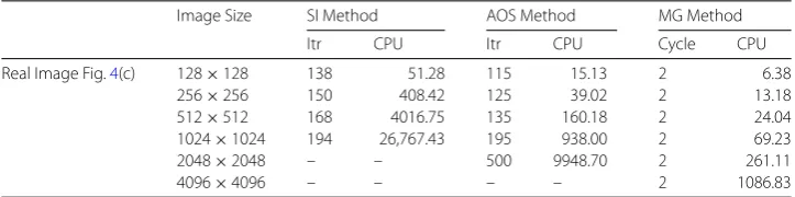
Table 2 Comparison of the proposed multigrid method (4.3) with SI (4.1), AOS (4.2) in terms of iterations and CPU time for an image with different sizes

Image Size SI Method AOS Method MG Method

Itr CPU Itr CPU Cycle CPU

Real Image Fig.4(c) 128×128 138 51.28 115 15.13 2 6.38

256×256 150 408.42 125 39.02 2 13.18

512×512 168 4016.75 135 160.18 2 24.04

1024_×1024 194 26,767.43 195 938.00 2 69.23

2048×2048 – – 500 9948.70 2 261.11

4096×4096 – – – – 2 1086.83

results of the proposed model are given in terms of the number of iterations, CPU time, and JSI. Clearly the proposed model is taking fewer iterations and converges fast with better JSI. Image size used in all experiments is 256×256 and the numerical method used for the solution of PDE in the table is additive operator splitting (AOS).

We observe that all the methods become slow in convergence as we increase the size of an image. To tackle this issue, we have proposed multigrid (MG) method, whose results are given in Table2. In Table2, we have given the number of iterations and corresponding CPU time for images having different sizes and different methods. A real color image given in Fig.4(c) is used for all computations given in Table2. From the table, it can be observed that the MG method has produced very good results in terms of the number of cycles and CPU time.

Furthermore, in Fig.4, we have tested the proposed model on different types of synthetic and real images. These results show effectiveness of the proposed model in different types of synthetic and real images. Fig.4(b), (d) are final segmented results of natural images, Fig.4(f ), (h) are segmented results of synthetic or artificial images, Fig.4(j), (l) are seg-mented results of biological cell images, and Fig.4(n), (p) are segmented results of med-ical MR images. We observe that our model segments images with intensity variation or inhomogeneity efficiently in the objects like in Fig.4(e), (g), (p). It can also segment images having inhomogeneity in their background as in Fig.4(k).

6 Conclusion

(a) (b) (c) (d)

(e) (f ) (g) (h)

(i) (j) (k) (l)

(m) (n) (o) (p)

Figure 4Original images are in column 1 and column 3 and their respective segmented results using our proposed model are given in column 2 and column 4. Results of real images are given in 1st row, while those of synthetic, biological cells, and medical images are given in 2nd, 3rd, and 4th rows, respectively

Acknowledgements

The authors would like to express their gratitude to the editors and anonymous reviewers for their valuable suggestions, which substantially improved the standard of the paper.

Funding

Availability of data and materials Not applicable.

Competing interests

The authors declare that they have no competing interests.

Authors’ contributions

The authors equally contributed in the paper. All authors have read and approved the final manuscript.

Publisher’s Note

Springer Nature remains neutral with regard to jurisdictional claims in published maps and institutional affiliations.

Received: 7 October 2017 Accepted: 6 June 2018

References

1. Caselles, V., Kimmel, R., Sapiro, G.: Geodesic active contours. Int. J. Comput. Vis.22(1), 61–79 (1997)

2. Mumford, D., Shah, J.: Optimal approximations by piecewise smooth functions and associated variational problems. Commun. Pure Appl. Math.42(5), 577–685 (1989)

3. Cremers, D., Rousson, M., Deriche, R.: A review of statistical approaches to level set segmentation: integrating color, texture, motion and shape. Int. J. Comput. Vis.72(2), 195–215 (2007)

4. Chan, T.F., Vese, L.A.: Active contours without edges. IEEE Trans. Image Process.10(2), 266–277 (2001)

5. He, L., Peng, Z., Everding, B.: A comparative study of deformable contour methods on medical image segmentation. Image Vis. Comput.26(2), 141–163 (2008)

6. Caselles, V., Catté, F., Coll, T., Dibos, F.: A geometric model for active contours in image processing. Numer. Math.66(1), 1–31 (1993)

7. Chan, T.F., Sandberg, B.Y., Vese, L.A.: Active contours without edges for vector-valued images. J. Vis. Commun. Image Represent.11(2), 130–141 (2000)

8. Bresson, X., Esedoglu, S., Vandergheynst, P., Thiran, J.P., Osher, S.: Fast global minimization of the active contour/snake model. J. Math. Imaging Vis.28(2), 151–167 (2007)

9. Badshah, N., Chen, K., Ali, H., Murtaza, G.: Coefficient of variation based image selective segmentation model using active contours. East Asian J. Appl. Math.2(2), 150–169 (2012)

10. Weickert, J., Romeny, B.T.H., Viergever, A.: An efficient local Chan–Vese model for image segmentation. Pattern Recognit.43(3), 603–618 (2010)

11. Badshah, N., Chen, K.: Multigrid method for the Chan–Vese model in variational segmentation. Commun. Comput. Phys.4(2), 294–316 (2008)

12. Badshah, N., Chen, K.: On two multigrid algorithms for modeling variational multiphase image segmentation. IEEE Trans. Image Process.18(5), 1097–1106 (2009)

13. Zhang, K., Zhang, L., Song, H., Zhou, W.: Active contours with selective local or global segmentation: a new formulation and level set method. Image Vis. Comput.28(4), 668–676 (2010)

14. Cai, X.: Variational image segmentation model coupled with image restoration achievements. Pattern Recognit.

48(6), 2029–2042 (2015)

15. Mora, M., Tauber, C., Batatia, H.: Robust level set for heart cavities detection in ultrasound images. In: Computers in Cardiology, pp. 235–238. IEEE Comput. Soc., Los Alamitos (2005)

16. Ghaffar, F., Badshah, N., Islam, S.: Multigrid method for solution of 3d Helmholtz equation based on hoc schemes. In: Abstract and Applied Analysis, vol. 2014. Hindawi Publishing Corporation, New York (2014)