Research on Monobit Frequency Measurement Algorithm with Split radix FFT

Research on Monobit Frequency Measurement Algorithm

with Split-radix FFT

Peng-fei JI

_{, Qi FENG and Nai-chang YUAN}

National University of Defense Technology, Changsha, Hunan, 410073 China *Corresponding author

Keywords: Monobit, Split-radix fast fourier transform, Single signal dynamic range, Two signal instantaneous dynamic range, Quantification.

Abstract. This paper gives a new method to calculate the split-radix fast Fourier transform (SRFFT combining radix-2 FFT with radix-4 FFT) through quantifying the twiddle factors based on the real and imaginary parts of them. Compared with the existing algorithms, 2 main advantages from the proposed algorithm have been found. 1. The average dynamic range is increased by 2.34dB from the existing algorithms when SNR reaches 20dB. 2. The dynamic ranges of the proposed algorithm are all improved under different noise environment. The simulation results verify the better effectiveness of the proposed algorithm.

Introduction

With the fast development of radar technology, wideband and multi-tone digital receivers are required urgently. Thus, a kind of monobit receiver, whose concept comes from commercial GPS receivers, was designed. To get this kind of receivers, people eliminate multiplication in DFT by using low bits ADC and quantifying the kernel function of DFT [1]. One advantage of monobit receiver is its simple structure. Thus, much design can be implemented in one chip. Another advantage is the ability to detect multiple signals while conventional existing instantaneous frequency measurement (IFM) receivers can process only one signal. Then, B. Y. Tsui proposed 4-point kernel DFT and designed a monobit wideband receiver [1-4], which was fabricated on a single chip and the instantaneous dynamic range can be 5dB. Meanwhile, the analysis in [5] proved that the approximate kernel function does not affect the estimation of the correct frequency.

The monobit receiver with 4-point kernel DFT was analyzed both theoretically and experimentally in paper [6]. It was found out that because of low bits quantification of both kernel function and digitalization, the dynamic range of 4-point kernel DFT (FFT) is very poor. And windowing cannot improve this result. Further- more, paper [7] presented the optimization of a monobit FFT digital receiver using a genetic algorithm. But the effect is not obvious.

Thus, this paper presents a new method of quantifying twiddle factors based on split-radix fast Fourier transform (SRFFT combining radix-2 FFT with radix-4 FFT) [8]. Furthermore, we design several groups of experiments to compare the proposed algorithm with the conventional existing algorithm and analyze the performance of the proposed algorithm in detail.

Optimization of Monobit FFT

In order to improve the Dynamic Range (DR) and decrease the difficulty of design, we propose a multi-bit quantification algorithm based on split-radix fast Fourier transform (SRFFT).

Analysis of SRFFT

  -1 2 2 0 -1 4 4 0 -1 4 3 4 0

(2 ) [ ( ) ( )] ,0 1

2 2

3

(4 1) [ ( ) ( ) ( ) ( )] ,0 1

4 2 4 4

3

(4 3) [ ( ) ( ) ( ) ( )] ,0 1

4 2 4 4

N kn N n N n kn N N n N n kn N N n N N

X k x n x n W k

N N N N

X k x n jx n x n jx n W W k

N N N N

X k x n jx n x n jx n W W k

     _{     }    _{          }     _{          }  







/4 /2 3 /4 and /4 /2

3 /4 . Therefore, we try to eliminate the multiplication from SRFFT by quantifying the two kinds of twiddle factors ( and ). Different from the traditional monobit algorithm which just have to quantify kernel function, SRFFT needs to quantify two kinds of twiddle factors hierarchically. For example, a signal flow graph of N-point SRFFT should be divided into M stages ( 2 , 2, ∈ ). And all the twiddle factors of L-shaped butterfly from each stage have to be quantified. The process is very tedious. However, we notice that all the twiddle factors can be divided into several levels. And the twiddle factors from each level are nothing to do with the specific value of input, but about the number of input points of the level as N in and . We should notice that 0 , 1, 2, ⋯ , ⁄4 1. Therefore, the twiddle factors from the same levels have to be quantified once and can be reused. Then we just need to store 4 units of different approximate twiddle factors for lookup table.

Meanwhile, we find that the phases of twiddle factors ( and , 0 ⁄4 1) do not range from 0 to 2 .

Thus, 4 main features have been concluded as follow:

(1)All the twiddle factors can be separated into different levels.

(2)The actual values of the two twiddle factors have no relationship with value of input, but the number of input points of each level.

(3)The phrase of always ranges from 0 to ⁄2 (the fourth quadrant).

(4) , which means that the phase of is 3 times of the phase of and the phrase of always ranges from 0 to 3 2⁄ (the whole complex plane except the first quadrant).

(5)The amplitudes of the two kinds of twiddle factor are both 1.

According to the above features, we design the algorithm of quantifying the twiddle factors.

Quantification Design

N-point DFT operation applied to a sequence is defined as follows:

 

1

2 /

0

( ) N j kn N n

X k x n e 



 





(2) Existing monobit algorithms are to eliminate multiplication by quantifying the kernel function ( / _{). Actually, the method of this algorithm is quantifying the phase of kernel function.} However, the design of approximate kernel function looks very hard and it is not very easy to implement the algorithm by FPGA.

Different from the existing algorithm, we quantify the values of real and imaginary parts of the twiddle factors from SRFFT according to the features of them to attain two kinds of the approximate twiddle factors. Thus, we expand one ( ) of the two kinds of twiddle factors.

2

cos(2 / ) sin(2 / )

n j

n N

N

W e n N j n N



 



1_{( ) [ cos(2 / )] /}

R

G n round L n N L ₍₄₎

1_{( ) [ sin(2 / )] /}

I

G n  round L n N L ₍₅₎ where round denotes rounding to the nearest integer; is quantification factor ( 2 , ∈ ). Then, the numbers of the values of the real and imaginary part are both 2 1. From Eq. 4 and Eq. 5, one kind of approximate twiddle factors can be denoted by .

1 1 1

4( ) R( ) I( )

G n G n  jG n ₍₆₎

The method of quantifying is the same as . We use to denote them.

3

3

3 3 3

4

( ) [ cos(2 3 / )] /

( ) [ sin(2 3 / )] /

( ) ( ) ( )

R

I

R I

G n round L n N L

G n round L n N L

G n G n jG n

 

  



  



 _{ }



 

(7) We do not have to consider the quantification of twiddle factors when programming SRFFT by FPGA. Because they have been done and stored before programming. Once the approximate twiddle factors are needed by the calculation of SRFTT, we can extract the part we need from lookup table (LUT) which stores the whole twiddle factors according to the length of the data of current level.

For example, assume that the input of current level from SRFFT is N-point data. Then, the approximate twiddle factors we need are and :

1 1 1

4( ) [1, 4(1), , 4( / 4 1),0]

G n  G G N  ₍₈₎

3 3 3

4( ) [1, 4(1), , 4( / 4 1), ]

G n  G G N  j ₍₉₎ where is the length of input data of the current level. So we can obtain the corresponding values of approximate twiddle factors in accordance with the value of .

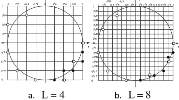
Assume 32, we can quantify the twiddle factors as shown in Figure 1, where we give two examples ( 4 and 8 ). In Figure 1, the black points show the results of the quantification of W and the white points are . We can see that the points are interleaved on the unit circle and the results of quantification are very close to the unit circle of complex plane. Furthermore, with the increase of , the results of the quantification with same input are closer to the unit circle. It means as Lis greater, the errors between the approximation and the original value are smaller.

a.  L 4       b.  L 8

Figure 1. Quantification of twiddle factors ( 32).

1 2

( ) m m

G n j

L L

 

(10) where n denotes the approximate twiddle factors, , ∈ , and , ∈ .

Then we can use the combination of shifting registers, adders and inverters to realize the binary multiplication in FPGA. Specific methods are shown in Table 1 [5].

Table 1. Binary Multiplication.

decimal multiplication binary multiplication

. . 101 0.1 10.1 . . 101 0.01 1.01 . . 101 0.11 10.1 1.01 11.11

Especially, additional bits ( log ) are needed to indicate the decimal during the quantification.

Experimental Results

To analyze the performance of the proposed algorithm, we design a series of experiments about 4-point kernel DFT, 12-point kernel FFT and the proposed algorithm through MATLAB. This section gives the results of the experiments.

Signal Parameters and Sampler

The specific parameters of experimental signal and sampler are shown in Table 2.

Table 2. Parameters of Experiments.

Signal Parameters

Number of Signal 1

Amplitude 1

Frequency Random, 125,1125 MHz

Primary phases Random, 0, 6.28 radian

Points of SRFFT 256

Signal Sampler

SNR 20dB

Sampling Frequency 2.5GHz

No. of ADC Bits 4

We added Hamming window into the input signal to optimize the results of experiments.

Results of Dynamic Range

Figure 2. Normalized-amplitude frequency response of 4-point kernel DFT and normal FFT.

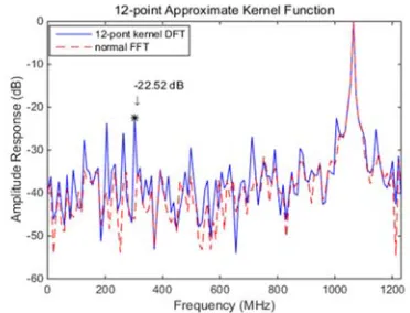
Figure 3. Normalized-amplitude frequency response of 12-point kernel DFT and normal FFT.

DFT is decreased by 21.23dB. The extent of the decrease is too high.

Then B. Y. Tsui gave the way of 12-point kernel FFT [5] to obtain improvement. And Figure 3 shows the frequency response of the 12-point kernel FFT. The frequency and primary phase of simulation signal is the same as in Figure 2.

Meanwhile, we use different values of L to get corresponding twiddle factors and give the frequency response of them as shown in Figure 4 (a), (b), (c) and (d). the quantification.

(a) L 1 (b) L 2

(c) L 3 (d) L 4

Figure 4. Normalized-amplitude frequency response of the proposed algorithm with different L and normal FFT

Average Dynamic Ranges under Different Signal-to-noise Ratios 

In order to eliminate the effects of noise and exceptions in above experiments, we conducted another group of experiment. Considering the results of section B, we calculated SRFFT with L=4 as reference and examples (we should notice that when L=4, we need at least 4 bits to denote a twiddle factor, which are the same to approximate kernel function in [5] ). The specific experimental method is as follows:

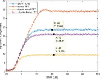
Change signal-to-noise ratio of experimental signal, SNR=-20:2:100 dB, and Calculate dynamic ranges of 4-point kernel DFT, 12-point kernel FFT and proposed algorithm (SRFFT, L=4) for 1000 times respectively. Signal parameters and sampler are shown in Table 2. Especially, the frequency of generated signal is random each time.

12-point kernel FFT and proposed algorithm (SRFFT, L=4) all keep steady as 9.5dB, 21dB and 23.5dB. Furthermore, when SNR 20 , we calculate the average dynamic ranges of them and normal FFT as: 9.46dB, 20.65dB, 23.22dB and 31.14dB. And the average dynamic range of SRFFT (L=4) is higher than the other algorithms and 2.34dB higher than 12-point kernel FFT.

Figure 5. Average dynamic ranges of 4-point kernel DFT, 12-point kernel FFT proposed algorithm (SRFFT, L=4) and normal FFT under different signal-to-noise ratios.

Conclusion

Based on the above analysis of the experiments and simulation in III, the proposed algorithm can suit modern receiver very well. Finally, because the proposed algorithm need less hardware, we can increase the value of quantification factor (L) to get higher dynamic range and larger instantaneous dynamic range without affecting the minimum hardware and processing requirements of digital receiver.

Therefore, the proposed multi-bit quantification algorithm based on Split-Radix FFT can meet the requirements of modern electronic warfare to be used for a broadband monobit receiver.

References

[1] J.B.Y. Tsui, Digital Techniques for Wideband Receiver, 2nd ed. Norwood, MA: Artech House, 2001.

[2] J.B.Y. Tsui, J. J. Schamus and D.H. Kaneshiro, "Monobit receiver," 1997 IEEE MTT-S International Microwave Symposium Digest, Denver, CO, USA, 1997, pp. 469-471 vol.2.

[3] D.S.K. Pok, C.I.H. Chen, J.J. Schamus, C.T. Montgomery and J.B.Y. Tsui, “Chip Design for Monobit Receiver,” IEEE Transactions on Microwave Theory and Techniques, vol. 45, no. 12, pp. 2283-2295, Dec 1997.

[4] J.B.Y. Tsui, D.H. Kaneshiro, and J.J. Schamus, ”Monobit Kernel Function Electronic Warefare Receiver for Characterizing Two Input Signals,” U.S. Patent US5963164.

[5] C.I.H. Chen, K. George, W. McCormick, J.B.Y. Tsui, S. L. Hary and K.M. Graves, "Design and performance evaluation of a 2.5-GSPS digital receiver," in IEEE Transactions on Instrumentation and Measurement, vol. 54, no. 3, pp. 1089-1099, June 2005.

a genetic algorithm," Proceedings of the 2004 IEEE Radar Conference (IEEE Cat. No.04CH37509), 2004, pp. 503-507.