Statistical Machine Learning Methods for the Large Scale Analysis of Neural Data

the Large-Scale Analysis of Neural Data

Gonzalo Esteban Mena

Submitted in partial fulfillment of the requirements for the degree

of Doctor of Philosophy

in the Graduate School of Arts and Sciences

COLUMBIA UNIVERSITY

Gonzalo Esteban Mena All Rights Reserved

Statistical Machine Learning Methods for

the Large-Scale Analysis of Neural Data

Gonzalo Esteban Mena

Modern neurotechnologies enable the recording of neural activity at the scale of entire brains and with single-cell resolution. However, the lack of principled approaches to extract structure from these massive data streams prevent us from fully exploiting the potential of these technologies. This thesis, divided in three parts, introduces new statistical machine learning methods to enable the large-scale analysis of some of these complex neural datasets. In the first part, I present a method that leverages Gaussian quadrature to accelerate inference of neural encoding models from a certain type of observed neural point processes — spike trains — resulting in substantial improvements over existing methods.

The second part focuses on the simultaneous electrical stimulation and recording of neurons using large electrode arrays. There, identification of neural activity is hindered by stimulation artifacts that are much larger than spikes, and overlap temporally with spikes. To surmount this challenge, I develop an algorithm to infer and cancel this artifact, enabling inference of the neural signal of interest. This algorithm is based on a a bayesian generative model for recordings, where a structured gaussian process is used to represent prior knowledge of the artifact. The algorithm achieves near perfect accuracy and enables the analysis of data hundreds of time faster than previous approaches.

The third part is motivated by the problem of inference of neural dynamics in the worm C.elegans: when taking a data-driven approach to this question, e.g., when using

whole-canonical neural identities, in practice resolved by tedious human labor. Alternatively, on a bayesian setup this problem may be cast as posterior inference of a latent permutation. I introduce methods that enable gradient-based approximate posterior inference of permutations, overcoming the difficulties imposed by the combinatorial and discrete nature of this object. Results suggest the feasibility of automating neural identification, and demonstrate variational inference in permutations is a sensible alternative to MCMC.

List of Figures v

1 Introduction 1

1.1 Summary of contributions . . . 4

I

Neural Coding Inference

8

2.2 A direct quadrature method for approximating the continuous-time log-likelihood in refractory models . . . 11

2.3 Application to generalized linear models . . . 15

II

Electrical Stimulation of the Retina

19

3.2 Materials and Methods . . . 23

3.2.1 Modeling neural activity . . . 26

3.2.2 Stimulation Artifacts . . . 26 3.2.3 A structured Gaussian process model for stimulation artifacts 29

3.2.5 Simplifications and extensions . . . 43

3.3 Results . . . 45

3.3.1 Algorithm validation . . . 45

3.3.2 Applications: high resolution neural prosthesis . . . 50

3.4 Discussion . . . 52

3.4.1 Simplified vs. full kernel-based estimators . . . 52

3.4.2 Comparison to other methods . . . 53

3.4.3 Online data analysis . . . 54

3.4.4 Limitations . . . 55

III

Identity inference in C.elegans

67

4.2 Background . . . 70

4.2.1 Definitions and notation. . . 70

4.2.2 Related Work . . . 70

4.2.3 Variational inference and the reparameterization trick . . . 71

4.3 Variational permutation inference via reparameterization . . . 74

4.3.1 Stick-breaking transformations to the Birkhoff polytope . . . . 74

4.3.2 Rounding toward permutation matrices . . . 77

4.3.3 Theoretical considerations . . . 78

4.4 Synthetic Experiments . . . 80

4.5 Brain dynamics of C. elegans . . . 82

4.6 Conclusion . . . 86

5 Learning Latent Permutations with Gumbel Sinkhorn Networks 87

5.2 The Sinkhorn operator: an analog of the softmax for permutations . . 89

5.3 Sinkhorn Networks . . . 91

5.3.1 Permutation equivariance . . . 92

5.3.2 Summary . . . 93

5.4 Probabilistic aspects: the Gumbel-Sinkhorn and Gumbel-Matching distributions . . . 94

5.4.1 Approximate Posterior Inference. . . 96

5.5 Experiments . . . 97

5.5.1 Sorting numbers . . . 97

5.5.2 Jigsaw Puzzles . . . 99

5.5.3 Assembly of arbitrary MNIST digits from pieces . . . 101

5.5.4 Posterior inference over permutations with the Gumbel-Sinkhorn estimator . . . 103

5.6 Discussion . . . 105

Bibliography 106 Appendix A Supplemental Information for Chapter 3 128 A.1 Experimental procedures . . . 128

A.2 Dataset details . . . 130

A.3 Kronecker product properties . . . 136

Appendix B Supplemental Information for Chapter 4 144 B.1 Alternative methods of discrete variational inference . . . 144

B.1.1 The Gumbel-softmax method . . . 145

B.1.2 Stick-breaking . . . 146

B.1.3 Rounding . . . 147

B.1.4 Limit analysis for stick-breaking . . . 149 B.1.5 Variational Autoencoders (VAE) with categorical latent variables150

B.2.1 Continuous prior distributions. . . 151

B.2.2 Computing the ELBO . . . 152

B.3 Experiment details . . . 155

Appendix C Supplemental Information for Chapter 5 157 C.1 Proof of Theorem 1 . . . 157

C.1.1 An approximation theorem for the matching problem . . . 159

C.1.2 Relation to softmax. . . 162

C.1.3 Illustrating theorem 1 . . . 162

C.2 Supplemental Methods . . . 163

C.2.1 Experimental protocols . . . 163

C.2.2 Number of parameters on Sinkhorn Networks . . . 164

C.2.3 Inference with the implicit Gumbel-Sinkhorn distribution . . . 165

C.3 Supplemental Results . . . 166

C.3.1 Puzzles. . . 166

C.3.2 Transformations into arbitrary digits . . . 167

C.3.3 Results on categorial VAE in MNIST . . . 168

C.3.4 Supplementary results on C.elegans . . . 169

C.4 Supplementary discussion . . . 170

C.4.1 Sinkhorn operator for approximate marginal inference . . . 170

C.4.2 Summary of extensions . . . 171

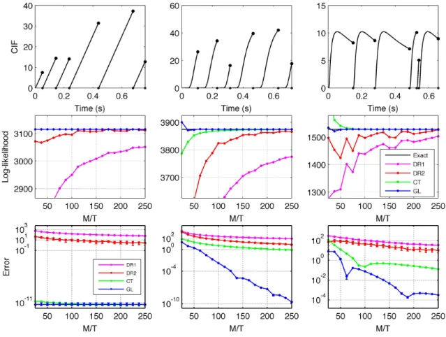
2.1 Comparing the four different likelihood approximation methods on three example renewal processes with absolute refractory periods ofτ = 2 ms. Left column: the ISI distribution was given by a Rayleigh distribution shifted by τ, with scale σ = ₁₀1q_π2. Center column: Inverse gaussian, meanµ= ₁₀1 and shapeλ= 1. Right column: Log-normal, shapeσ = 1, and log-shape µ=−2.5. Top row: CIF during the first six spikes of a single trial. Note that the CIF falls to zero after each spike. Parameters were chosen so that all the mean firing rates were between 10 and 15 Hz. Middle row: One sample of the approximated log-likelihood as a function of M/T, the total number of CIF evaluations per second, for each of the four methods (the two discrete time approximations, DR1 and DR2, the continuous time approximation based on Riemann sums, CT, and the Gauss-Lobatto quadrature method, GL). Bottom row: Median and quartiles of the absolute approximation error as a function of M/T (note log scale). The first plotted value of M s−1 is roughly the smallest for which it is possible to distribute Mmin= 3 CIF evaluation points (not including ti+τ, where the CIF is known to be

zero) into each integral. The GL approach clearly produces the best results. . . 16

ent methods. A spike train was sampled for T = 40s with CIF given by λ(t|Ht) = exp(θ1sin(4πt) + θ2)r(t − tN(t)−) with r(t) =

max(0,min(_τ1

2(t − τ1),1)), τ1 = 2ms, τ2 = 10ms, θ = (3,2). Left:

CIF during the first ten spikes. Center and Right: Maximum likelihood approximate solutions of θ1 and θ2 using the different methods, for different values ofM/T. . . 17

3.1 Overlapping electrical images of 24 neurons (different colors) over the MEA, aligned to onset of spiking att = 0.5ms. Each trace represents the time course of voltage at a certain electrode. For each neuron, traces are only shown in the electrodes with a strong enough signal. Only a subset of neurons visible on the MEA are shown, for better visibility. . . 22 3.2 Visual inspection of traces reveals the difficulty of the problem.

First column: templates of spiking neurons. Second to fourth columns: responses of one (A) or two (B) cells to electrical stimulation at in-creasing stimulation amplitudes as recorded in the stimulating electrode (first rows) or a neighboring, non-stimulating electrode (third rows). If the stimulation artifact is known (gray traces) it can be subtracted from raw traces to produce a baseline (second and fourth rows) amenable for template matching: traces with spike(s) (colored) match, on each electrode, either a translation of a template (A andB) or the sum of different translations of two or more templates (B). As reflected by the activation curves (fifth column) for strong enough stimuli spiking occurs with probability close to one, consistent with the absence of black traces in the rightmost columns. . . 25

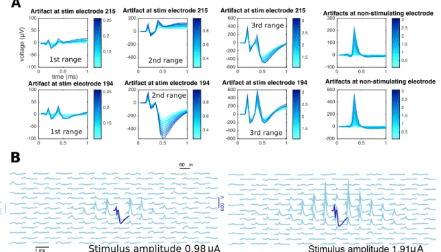
TTX experiments. (A) local, electrode-wise properties of the stim-ulation artifacts. Overall, magnitude of the artifact increases with stimulation strength (different shades of blue). However, unlike non-stimulating electrodes, where artifacts have a typical shape of a bump around 0.5 ms (fourth column), the case of the stimulating electrode is more complex: besides the apparent increase in artifact strength, the shape itself is not a simple function of stimulating electrode (first and second rows). Also, for a given stimulating electrode the shape of the artifact is a complex function of the stimulation strength, changing smoothly only within certain stimulation ranges: here, responses to the entire stimulation range are divided into three ranges (first, second, and third column) and although traces within each range look alike, traces from different ranges cannot be guessed from other ranges. (B) stimulation artifacts in a neighborhood of the stimulating electrode, at two different stimulus strengths (left and right). Each trace represents the time course of voltage at a certain electrode. Notice that stimulating electrode (blue) and non-stimulating electrodes (light blue) are plotted in different scales. . . 27

in the top, center, and bottom rows, respectively. Center: correspond-ing stationary auto-covariances from the Matérn(3/2) kernels (Eq 3.4).

Right: corresponding unnormalized ‘gamma-like’ envelopes dα,β (Eq

3.5). The inferred quantities are in agreement with what is observed in Fig 3.3B: first, the shape of temporal termdα,β reflects that the artifact

starts small, then the variance amplitude peaks at ∼.5 ms, and then decreases rapidly. Likewise, the corresponding spatial dα,β indicates

that the artifact variability induced by the stimulation is negligible for electrodes greater than 700 microns away from the stimulating elec-trode. BSame as A), but for the stimulating electrode. Only temporal kernels are shown, for two inter-breakpoint ranges (first and second rows, respectively). . . 37 3.5 Example of neural activity and artifact inference in a

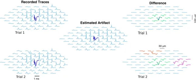
neigh-borhood of the stimulating electrode. Left: Two recordings in response to a 2.01 µAstimulus. Center: estimated artifact (as the stim-ulus doesn’t change, it is the same for both trials). Right: Difference between raw traces and estimated artifact, with inferred spikes in color. In the first trial (above) one spiking neuron was detected, while in trial 2 (below) three spiking neurons were detected. The algorithm separates the artifact A and spiking activity s effectively here. . . 46

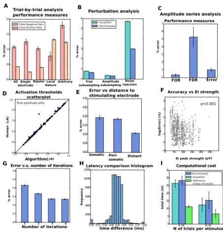
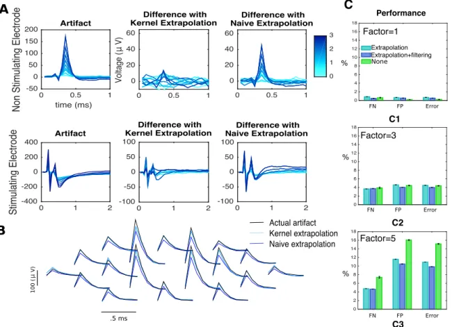
the efficacy of the algorithm A. Trial-by-trial wise performance of estimators broken down by the the four types of stimulation considered (total number of trials 1,713,233, see Table A.1 in the Appendix for details). B. Trial-by-trial wise performance of estimators to perturba-tions of real data (only single-electrode): five trials per stimulus for trial subsampling, every other stimulus for amplitude subsampling and σ= 20 for noise injection. C,D. Amplitude-series wise performance of estimators. C: false omission rate (FOR = FN/(FN+TP)), false dis-covery rate (FDR = FP/(FP+TP)), and error rate based on the 4,045 available amplitude series (see Table A.2 in the Appendix for details);D: comparison of activation thresholds (human vs. kernel-based algorithm). E. Performance measures (trial-by-trial) broken down by distance be-tween neuron and stimulating electrode. F. Trial-by-trial error as a function of EI peak strength across all electrodes (only kernel-based). A Spearman correlation test revealed a significant negative correlation. G. Error as a function of number of iterations in the algorithm. H. For the true positives, histogram of the differences of latencies between human and algorithm. I. Computational cost comparison of the three methods for the analysis of single-electrode scans, with 20 to 25 (left) or 50 (right) trials per stimulus. . . 60

tifact estimate in our simulations. Aeffect of filtering on traces for two non-stimulating electrodes, at a fixed amplitude of stimulation (2.2µA). A1,A3 raw traces,A2,A4 filtered traces. Notice the two main features of the filter: first, it principally affects traces containing spikes, a consequence of the localized nature of the kernel in Eq 3.2. Second, it helps eliminate high-frequency noise. Bthrough simulations, we showed that filtering leads to improved results in challenging situations. Two fil-ters — only smoothing and localization + smoothing — were compared to the omission of filtering. In all cases, to rule out that performance changes were due to the extrapolation estimator, extrapolation was done with the naive estimator. B1 results in a less challenging situation.

B2 results in the heavily subsampled (nj = 1) case. B3 results in the

high-noise variance (σ2 _{= 10) case. . . . . 61}

initial estimates of the artifact. A comparison between kernel-based extrapolation and the naive estimator, the artifact at the previous amplitude of stimulation. For a non-stimulating (first row) and the stimulating (second row) electrode, left: artifacts at different stimulus strengths (shades of blue), center: differences with extrapolation estima-tor (Eq 3.11), right: differences with the naive estimaestima-tor. Bcomparison between the true artifact (black), the naive estimator (blue) and the kernel-based estimator (light blue) for a fixed amplitude of stimulus (3.1µA) on a neighborhood of the stimulating electrode. C Through simulations we showed that extrapolation leads to improved results in a challenging situation. Kernel-based extrapolation was compared to naive extrapolation. C1 results in a less challenging situation. C2-C3

results in the case where the artifact is multiplied by a factor of 3 and 5, respectively.. . . 62 3.9 Analysis of responses of neurons in a neighborhood of the

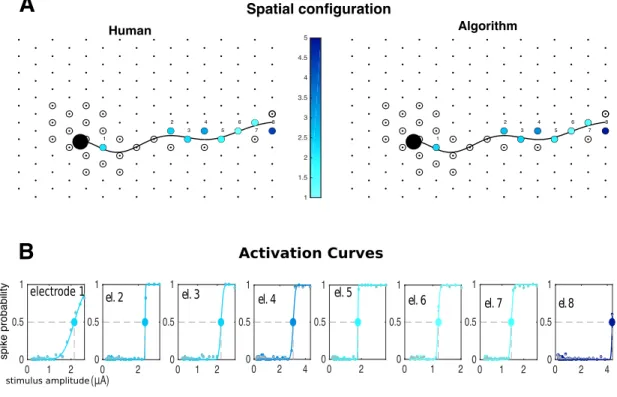
stimulating electrode. ASpatial configuration: stimulating electrode (blue/yellow annulus) and four neurons on its vicinity. Soma of green neuron and axon of pink neuron overlap with stimulating electrode. B Activation curves (solid lines) along with human-curated and algorithm inferred spike probabilities (gray and colored circles, respectively) of all the four cells. Stimulation elicited activation of green and pink neurons; however, the two other neurons remained inactive. CRaster plots for the activated cells, with responses sorted by stimulation strength in the y axis. Human and algorithm inferred latencies are in good agreement (gray and colored circles, respectively). Here, direct somatic activation of the green neuron leads to lower-latency and lower-threshold activation than of the pink neuron, which is activated through its axon. . . 63

the soma (black circle) and axon (black line) over the array. Electrodes where stimulation was attempted are represented by circles, with colors indicating the activation threshold in the case of a successful activation of the neuron within the stimulation range. BFor those cases, activation curves (solid lines) are shown along with with human and algorithm inferred spike frequencies (gray and colored circles, respectively). Large circles indicate the activation thresholds represented in A. In this case, much of the activity is elicited through axonal stimulation, as there is a single electrode close to the soma that can activate the neuron. Human and algorithm are in good agreement. . . 64 3.11 Analysis of differential responses to single (A) and two-electrode

(B) stimulation. Gray and colored dots indicate human and algorithm inferences, respectively. In both cases activation of the two neurons is achieved. However, shape of activation curves is modulated by the presence of a current with the same strength and opposite polarity in a neighboring electrode (yellow/blue annulus inB): indeed, in this case bipolar stimulation leads to an enhanced ability to activate the pink neuron without activating the green neuron. The algorithm is faithfully able to recover the relevant activation thresholds. . . 65

sol cells. For each neuron, one or more stimulating electrodes in a neighborhood of neural soma were chosen for stimulation. AReceptive fields colored by the lowest achieved stimulation threshold (black if activation was not achieved). BInferred somas (big black circles) of the neurons labeled A-E inA), showing which electrodes were chosen for stimulation (small circles) and whether activation was achieved (colors). C Activation curves (solid lines) of the neurons in B for the successful activation cases. Gray and colored dots represent human and algorithm results, respectively, and large circle indicates stimulation thresholds. 66

4.1 Reparameterizations of discrete polytopes. From left to right: (a) The Gumbel-softmax, or “Concrete” transformation maps Gumbel r.v.’sψ ∈_RN

(blue dots) to points in the simplexx∈∆N by applying the softmax.

Colored dots are random variates that aid in visualizing the transfor-mation. (b) Stick-breaking offers and alternative transformation for categorical inference, here from points β ∈ [0,1]N−1 to ∆N, but the

ordering of the stick-breaking induces an asymmetry in the transforma-tion. (c) We extend this stick-breaking transformation to reparameterize the Birkhoff polytope, i.e. the set of doubly-stochastic matrices. We show how B3 is reparameterized in terms of matrices B ∈ [0,1]2×2 These points are mapped to doubly-stochastic matrices, which we have projected onto _R2 below (stencils show permutation matrices at the vertices). (d) Finally, we derive a “rounding” transformation that moves points in_RN×N nearer to the closest permutation matrix, which is found with the Hungarian algorithm. This is more symmetric, but does not map strictly ontoBN. . . 72

match squares to circles. (a) Examples of center locations (circles) and noisy samples (squares), at different noise variances. (b) For illustration, we show the true and inferred probability mass functions for different method (rows) along with the Battacharya distance (BD) between them for a selected case of eachσ(columns). Permutations (indices) are sorted from the highest to lowest actual posterior probability. Only the 10 most likely configurations are shown, and the 11st bar represents the mass of all remaining configurations. (c) KDE plots of Battacharya distances for each parameter configuration (based on 200 experiment repetitions) for each method and parameter configuration. For comparison, stick-breaking, rounding, and Mallows (θ= 1.0) have BD’s of .36, .35, and .66, respectively, in the σ= 0.5 row of (b). . . 79 4.3 Inferring labels and weights in C. elegans. (a) Neural activity is

optically recorded in genetically modifiedC. elegans. (b) The output is a multivariate time series of neural activity of N neurons for each worm. (c) The first challenge is to infer a latent permutation that matches observed neuron indices to the known set of neuron names, or labels. (d)The second challenge is to infer the weights with which each neuron influences its synaptic neighbors. The connectome (i.e. adjacency matrix) is known, but the weights are not. . . 82

vergence of the algorithm, and the baselines. (b) Accuracy of identity inference as a function of mean number of candidates (correlated with ν), for M = 1 worm (square) and combining information of M = 5 worms (circles). (c) Accuracy as a function of the proportion of known networks beforehand, with ν = 0.1 (circles) and ν = 0.05 (squares). (d)Variance of distribution over permutations (vectorized) as a function

of the number of iterations. (e) Two samples of permutation matrices

round(Ψ) (right) and their noisy, non-rounded versions Ψ (left) at the

twentieth algorithm iteration. The average of many samples is also shown. These averages take values in (0,1), indicating uncertainty in the variational posterior. . . 83

5.1 Schematic of Sinkhorn Network for Jigsaw puzzles. . . 93 5.2 (a) Sinkhorn networks can be trained to solve Jigsaw Puzzles. Given

a trained model, ‘soft’ reconstructions are shown at different τ using S(X/τ). We also show hard reconstructions, made by computingM(X) with the Hungarian algorithm [Munkres,1957a]. (b) Sinkhorn networks can also be used to learn to transform any MNIST digit into another. We show hard and soft reconstructions, withτ = 1. . . 101

A.1 ARaw artifact traces at the smallest amplitude of stimulation (0.1µA), considered an estimate of µ, the switching artifact. B Raw artifact traces at 0.99 µAof stimulus. C Difference. Notice that the main text refers to this already mean-subtracted artifact. D) Left: Raw artifact at all different stimuli for a non-stimulating electrode (inset, switching artifact). Right: Differences. . . 138

proposed inHashimoto et al.[2002] and our simplified estimator. These results complement figure 3.6A, by reporting differences by type of estimator, and also by reporting total errors. . . 139 A.3 Comparison of simplified and kernel-based estimator in the

analysis of perturbations to real data. These results complement figure 3.6B, by reporting false positive and negative rates at different conditions for trial subsampling (top), amplitude subsampling (middle) and noise injection (bottom). Only for single electrode stimulation. Notice that for trial sub-sampling and noise injection, results may vary from one experiment to another. . . 140 A.4 Distribution of EI strength on the stimulating electrode among spike

events, both for somatic and axonal (distant) stimulation. For somatic stimulation inset corresponds to a zoom to smallest voltages. For EI peak strengths smaller than 10µV spike is not observed (based on manual analysis). . . 141 A.5 Population based estimates of the mean (top) and standard deviation

(bottom) of spike latency, as a function of probability of spiking (left) and stimulus amplitude (right). This supports the observation that when activation is reached (high probability of spike) variability of latencies reaches its minimum. . . 142

phenomenological model for two electrode stimulation. Obser-vations are based on a single retinal preparation (TTX). A)example of observed linearity: A1-A2) artifacts for single electrode stimulation at two different stimulating electrodes with same strength (3.1 µA) and opposite polarities. A3) corresponding two-electrode stimulation. A4) sum of A1) andA2). A5) difference between A3) andA4). A6) for reference, the EI of a typical neuron in shown in the same scale. B) population-based generalization of the finding in A)from thousands of stimulating electrode pairs, collapsing stimulating amplitudes and elec-trodes. B1-B2) scatterplots of the maximum strength (over electrodes and time) of two-electrode stimulation artifacts at different stimulus strengths (strength of the color) before and after subtracting the sum of single electrode artifacts. Points in the gray-scale are the ones shown in A). B3 histogram of log peak EI of neurons in the array. In the light of B3, B1,B2 show in the vast majority of artifacts of magnitude comparable with than of EI ( 99% of points above the diagonal and outside the log-strength 2.5 µV boxes in B1,B2) subtracting the linear sum of individual artifacts is a sensible choice as it decreases its strength.143

B.1 Examples of true and reconstructed digits from their corresponding discrete latent variables. The real input image is shown on the left, and we show sets of four samples from the posterior predictive distribution for each discrete variational method: Gumbel-softmax, rounding, and stick-breaking. Above each sample we show the corresponding sample of the discrete latent “code.” The random codes consist of of K = 20 categorical variables with N = 10 possible values each. The codes are shown as 10×20 binary matrices above each image. . . 152

Matching and Gumbel-Sinkhorn distributions. Each 5x5 grid represents a matrix, with the shading indicating cell values (a) Matching opera-tor M(X) applied to a parameter matrix X. (b) Sinkhorn Operator S(X/τ) approximating M(X) for different temperatureτ and number of Sinkhorn iterations, L. (c). First row: samples from the Match-ing Sinkhorn distribution. Second and third rows: samples from the Gumbel-Sinkhorn distribution at two temperatures. At low tempera-ture, both distributions are indistinguishable. . . 163 C.2 First column: samples from dataset created by mixing all pieces of digits,

and then re-assembling them into ‘digits’. Second column: random permutations of first column. Third column: hard reconstructions using M(X). Fourth column: soft reconstructions using S(X/τ) and τ = 1. Metaphorically, one is able to reconstruct pieces out of ‘dust’.. . . 168

Firstly, I would like to thank my advisor Liam Paninski for his willingness to be my mentor, and for having trusted that I was going to be able to solve such relevant (but complicated) computational problems. I came to Columbia with a background in math, a strong interest in neuroscience but no experience. So it was definitely mind-blowing when in our first meetings he started sayings things like ‘let ni, i = 1, . . . n be n

neurons’. Putting my hands in data was a bit of a shock at first. But know, after years of seeing data, I am proud of having learned how to deal with massive data using advanced math, it is the superpower that I learned at Columbia, thanks to Liam and his school. It has been a tremendous luxury to have regular him for regular interactions to learn from his scientific wisdom, or just to laugh.

Thanks also to John Cunningham, who while not officially my advisor has also acted

de facto as such, showing genuine commitment to help. I can also say I learned a

lot from him, particularly from his Gaussian processes class and his advocacy for maximum entropy methods.

Thanks to EJ Chichilnisky and his Lab (particularly, Lauren Grosberg, Nishal Shah and Sasi Madugula) for giving me access to the unique and gorgeous data they produce, and for letting me helping them in overcoming their technical hurdles. Joining EJ’s revolutionary project has been such an adventure for me; I will always remember the times I visited his amazing lab and was there in the late experiments seeing retinal responses on the board; I felt I was participating on a NASA rocket launch!

I am thankful of having met David Blei, who influenced me to commit to the project

progress. Dave’s reading group is the place I learned the most at Columbia, and I am also thankful of all participants, with whom we generated many insights.

I thank the members Andrew Gelman and John Paisley, for generously agreeing to read and evaluate this work.

Thanks also to the great students and postdocs that I have met at Columbia, with whom I interacted in the entire spectrum, from collaboration to just hanging out. Particularly, Scott Linderman, Jaan ‘el estonio’ Altosaar, Francisco Rodriguez, Adji Dieng, Francisco J. R. Ruiz, Ella Batty, Ari Pakman, Mariano Gabitto, Yuanjun Gao, Peter Lee, Kelly Buchanan, Dar Gilboa, Morgane Austern and John Auerbach.

I am grateful with Jasper Snoek for believing I was a good choice for a summer internship at Google Brain. It was super fun to use neural networks to solve puzzles using many GPUs.

I thanks to my roommates Gonzalo Munoz, Francisca Cabanas and Mauro Escobar for accepting being my roommates.

I also want to express my gratitude to the entire Columbia Department of Statistics, staff, and my fellow graduate students. In particular, I would like to thank Peter Orbanz and Phillip Protter for career advice and always being available to talk about any topic. I would also like to thank Dood and Anthony for assisting me with anything and everything.

I thank my friends in Chile Felipe Tobar and Joaquin Fontbona who generously invited me every year to give talks about preliminary research results.

Lastly, I would like to thank my family (Manuel, Javiera, Cristian and Sonia) for their love. This thesis is for you.

Chapter 1

Introduction

According to our reductionist view of the world, to understand how the mind arises and works we need to understand the functioning of its atomic components, which are largely believed to be neurons. Neurons are so small that we cannot see them, and their physiological processes occur at much faster time-scales than the ones at which we do make sense of the world. Therefore, such modern reductionist scientific study of the mind is impossible without the use of ad-hoc technologies that enable our access to such scales.

The need count with suitable recording or imaging methods has been a primary preoccupation for neuroscientists in the past 130 years, and their development and use has underlied scientific milestones. A first notable example is given by Ramon y Cajal, whose main contributions arose from the refinement of Golgi’s staining technique, enabling the discovery of dendritic spines [Yuste, 2015a], thus suggesting the discreteness of neurons and laying the basis for the conception of the still dominating

doctrine of the neuron 1,2_{. Another last-century example is given by the invention of} the Tunsgsten electrode by Hubel [Hubel et al.,1957] that enabled precise single-unit recordings. Huber and Wiesel’s experiment in the cat (e.g. [Hubel and Wiesel, 1962]) greatly profited from this enhanced resolution and eventually paved the way for the development of the theory of receptive fields, through which we understand (some) neurons as units ofperception [Barlow,1972,Yuste,2015b] that organize hierarchically; from crude photon reception at the retinal level, to abstract conceptual representation in higher order areas.

Although the drive for scientific discovery remains untouched, our times are unique because of the development of several high-throughput imaging methods that grant us with access to more refined spatio-temporal scales, but more importantly, to the recording of large volumes of neural tissue comprising up thousands of neurons, with exquisite single neuron resolution. This sudden shift in scales has already allowed experimentalist to record neural activity of entire brains and nervous systems, as with

the C.elegans [Nguyen et al., 2016a] the Larval Zefrafish [Ahrens et al., 2013] and

the Hydra [Dupre and Yuste,2017]. As a result, new fundamental knowledge on how

the mind works (i.e. relation between behavior, whole-brain neural dynamics and environmental variables) have been obtained in these small animals, and this is only the beginning.

Further, recently developed neural stimulation technologies have showed promising

1_{Anecdotally, to communicate his results with the scientific community, Ramon y Cajal had to}

make drawings of what he observed in the microscope, in the lack of suitable microscopic photography methods. Because of their historic relevance and aesthetic content, these drawings are still greatly appreciated today.

2_{It was not only until the fifties, with the development of the electron microscope, that the}

discreteness of neurons theory was tested empirically [Yuste,2015b]. Surprisingly, in the dawn of artificial intelligence, researchers were already ‘experimenting’ with this non-validated theory already at least a decade before.

success to enable the stimulation of groups of neurons also at single cell resolution, and in large-scale setups. This, in turn, opens the doors for the development of methods

tocontrol the activity of neural populations, a principle of tremendous scientific and

clinical significance, as stated in the BRAIN initiative report [Bargmann et al., 2014]. Scientifically, to study functional relationships among neurons by perturbing neural circuits at will. Clinically, for the development of prosthesis and other therapies to treat neurological, psychiatric and neurodegenerative disorders: since current prosthetic devices to e.g. treat loss of audition (cochlear implant) and for movement restoration have shown reasonable success [Lebedev and Nicolelis, 2017] even if they currently act at a extremely low resolution, it is reasonable to believe much more could be achieved if such control was achieved at the scale of thousands, or millions of neurons, and in closed-loop.

However, the goodness of these technologies comes at the cost of new challenges: the data stream that can be routinely recorded these days is in the order of terabytes per day, so even storing that information is non-trivial [Sejnowski et al., 2014,Freeman,

2015, Landhuis, 2017]. More generally, to extract any meaningful information from data (e.g. finding action potentials, inferring the low-dimensional manifold where neural activity lies, etc), a large-scale statistical analysis has to be performed. Further, the big-data quantities involved in these analysis will often challenge our statistical common-sense on to how to test hypothesis arising from the obtained information, but at the same time will enable the formulation of new hypothesis that would not been possible previously [Gao and Ganguli, 2015, Pillow and Aoi, 2017,Elsayed and Cunningham,2017].

Because of the scientific and societal relevance of the large-scale neuroscience program, people have recently advocated for the conceptualization of a new field, neural data

science [Paninski and Cunningham, 2017], a discipline aimed to propose principled

solutions to these new challenges. This thesis falls within the scope of this new discipline; and it can be deemed as an attempt to solve specific computational

challenges arising from the use of new large-scale recording (orreading) an stimulation

(or writing) technologies in neuroscience. Further, because of the historical confluence

of this new age of neuroscience with the increased computational power and the achieved prominence of large-scale machine learning, this thesis can be also be framed within the scope of statistical machine learning: to surmount these challenges I use mathematical, statistical and computational principles to propose models for data, and to develop algorithms that efficiently perform inference in the models. Notably, although this work gravitates towards problem solving, the non-triviality of problems being tackled led to methodological advances in the field of statistical machine learning.

1.1

Summary of contributions

The the remainder is organized in three parts and four chapters. Each part corresponds to an individual research project, and each of chapters to a (published) research paper. While parts I andIIcontain an individual chapter, IIIcontains two (chapters4and 5) that explore different aspects of the project.

Part I (chapter 2), neural coding

The neural coding problem corresponds to determining which features of the world neurons respond to (encode). The standard data-driven approach consist on inferring a model that expresses the distribution of neural responses given stimuli time-series. These responses are represented as spike trains, and can be thought as the emissions of a point process. Therefore, efficient methods for inference in point processes are required. My contribution in this area [Mena and Paninski, 2014]3 was the discovery and implementation of a simplifying Gaussian quadrature approximation for the calculation of the mean firing rate that greatly facilitates its inference, providing

substantial improvements over existing methods. As a result, now we can fit neural encoding models much faster, without sacrificing accuracy.

Part II (chapter 3), electrical stimulation of the retina

In collaboration with EJ Chichilnisky lab at Stanford, I have extensively researched computational aspects to the problem of large-scale neural stimulation [Mena et al.,

2017]4_{. Specifically, our context is the use of multi-electrode arrays for the stimulation} recording and stimulation of neural activity in retinal ganglion cells. There, perva-siveness of stimulation artifacts stymies our ability to make sense of data: recordings in multi-electrode arrays in response to electrical stimuli are heavily corrupted, since stimuli are sensed in the electrodes as artifacts that are of much larger magnitude than true neural signals, and overlap in time with neural signals. Therefore, current approaches to infer neural responses in the large-scale analysis require painstaking manual curation by a highly skilled experimentalist. I invented a method that auto-mates this analysis: it enables a fast read-out of neural activity even in this highly corrupted regime. Briefly, it is based on assuming a bayesian generative model for recorded voltage traces, where a structuredgaussian process is used to represent our prior knowledge of the artifact. This choice furnishes our methodology with a number of operations (extrapolation, filtering) that we implement in a efficient inference algorithm that accurately separates this contaminating signal from the neural signals of interest. The resulting algorithm greatly enhances the data analysis pipeline, as now it is possible to analyze in hours volumes of data (several terabytes) that would otherwise take months of human analysis.

Currently, we are applying this algorithm to prototype novel high-resolution neural prosthesis to treat loss of sight due to retinal degeneration. There, the algorithm allow us to rapidly infer how different stimulus do elicit responses on neurons, a type of

4_{Joint work with Lauren Grosberg, Sasi Madugula, Paweł Hottowy, Alan Litke, John Cunningham,}

information that is crucial for tailoring electrical stimuli that generates arbitrary visual perception. Naturally, this information is also useful in the purely scientific setup, to shed light in the biophysical process that mediate electrophysiological phenomena (e.g. action potentials, axonal activation) as a response to different kinds of electrical

stimuli.

Part III (chapters 4, 5), identity inference in C.elegans

The worm C. elegans is a peculiar animal: the number of neurons (302 in the hermaphrodite) does not change across specimens, nor does the connectome, its wiring diagram. This makes it a unique model organism for neuroscientists, as one can take a direct data-driven approach to probing the question of how the brain works, i.e., the dynamics that describe how past and current neural states relate drive future ones, while relate to sensory input and behavior. Experimentalists now can routinely record activity of each neuron in the worms, and our goal is to use this data to infer the underlying dynamics. We give a bayesian treatment to this problem: dynamics are assumed to come from a distribution that encodes our prior knowledge (e.g. the connectomic information), and are weighted against evidence (recordings). However, identity of each recorded time series is not know beforehand, and for meaningful inferences one needs to first solve the problem of matching recorded traces to canonical neural identities. In practice, inference of this matching requires painstaking human analysis.

We state this problem within our bayesian setup, by including a latent permutation, for which we seek to perform posterior inference. We appeal to variational inference as an alternative to the exact (but given our empirical findings in this case, slow) MCMC sampler. In detail: in variational inference one casts posterior inference as optimization, the one of finding the closest (here, in the sense of the Kullback-Leibler divergence) distribution within a parametric family. As the function to be optimized expresses as an expectation, gradient-based algorithms can be derived by appealing to

the theory of stochastic optimization. However, the use of permutations complicates the use of gradient-based methods: first, non-trivial families over permutations are described in terms of an intractable partition function. Second, as permutations are (non-differentiable) discrete objects, and usual gradient estimators for stochastic optimization cannot be applied. To alleviate this problem, we developed many relaxations (two in chapter 4, published as [Linderman et al., 2018]5 _{and a third in} chapter 5, published as [Mena et al., 2018] 6_{) that replace discrete permutations by} continuous approximations. The latter, that we named Gumbel-Sinkhorn proved the most successful, and is based on two ideas i) distributions in the variational families are reparameterized in terms of a noise distribution, as solutions of Gumbel-perturbed matching problem on the Birkhoff polytope, and ii) we conceive a differentiable approximation to the non-differentiable matching in terms of the so called Sinkhorn

operator, the solution to an entropy regularized version of the original problem. We showed our methods outperform the naive MCMC sampler in the neural identification task, indicating a great potential to improve current data-analysis capabilities by automatic procedure that otherwise would be extremely laborious for a human.

Finally, notice that chapter 5 also addresses the topic of the use of artificial neu-ral networks (ANN) for supervised learning of permutations (e.g. solving puzzles or sorting numbers), a slightly different problem than the original neural identity inference (where, no ANN is required). The main connecting narrative is the use of a differentiable approximation for permutations, provided by the Sinkhorn operator. It is this secondary ANN narrative that motivates the division of Part III into two chapters.

5_{Joint work with Scott Linderman, Hal Cooper, John Cunningham and Liam Paninski.}

6_{Joint work with David Belanger, Scott Linderman and Jasper Snoek. Most of this work was}

Part I

Chapter 2

Quadrature Methods for Refractory

Point Process

2.1

Introduction

Point processes are a powerful theoretical tool to characterize the occurrence of random events in time, and are widely used in statistical neuroscience [Truccolo, 2010] to represent neural spiking in terms of intrinsic factors, including refractoriness and the activity of other neurons, and extrinsic factors, such as stimulus-driven effects. One way to characterize such processes is through the conditional intensity function (CIF). Intuitively, the CIF can be interpreted as an instantaneous firing rate given the past history. This history, denotedHt, is meant to represent changes in spiking probabilities

due to previous activity, e.g., refractoriness. The log-likelihood of observing the spikes at times t1, . . . , tN(T) in the interval [0, T] is given by [Brillinger, 1988, Daley and

Vere-Jones,2008] l(t1, . . . tN(T)) = N(T) X i=1 log(λ(ti|Hti))− Z T 0 λ(t|Ht)dt, (2.1)

Usually, an explicit functional model of the CIF is assumed. The most popular approach involves generalized linear models (GLM) [Brillinger, 1988, Paninski,2004,

Truccolo, Eden, Fellows, Donoghue, and Brown, 2005], in which the CIF is a function of a linear transformation of the stimulus and other known covariate terms. This leads to a parametric expression for the likelihood, in which maximum likelihood (ML) or maximum a posteriori (MAP) estimates are computed using standard optimization methods that evaluate the log-likelihood (and derivatives) at each iteration. The main problem is that only approximations of the full continuous-time log-likelihood can be computed, as there may not be a closed form expression for the cumulative CIF, RT

0 λ(t|Ht)dt.

Previous approaches are based on discrete-time versions of the spiking process, which in turn lead to discretizations of the log-likelihood that converge to the continuous version when the bin size goes to zero. For point processes with refractory effects, in which the CIF jumps discontinuously to zero following a spike, [Citi, Ba, Brown, and Barbieri,2014] recently developed an improved such discretization. Here we show that an alternative approach, in which we apply standard quadrature methods directly to the original continuous time integral, leads to significant further improvements beyond those offered by the approach of [Citi et al., 2014], with minimal additional computational cost1_.

1_{Recently submitted independent work by K. Lepage makes a similar point [Lepage and MacDonald,}

2.2

A direct quadrature method for approximating

the continuous-time log-likelihood in refractory

models

To begin, it is useful to discuss both the standard discretization approach and also the more refined method of [Citi et al., 2014]. Both of these approaches begin by discretizing the observed continuous-time spike train process{ti}into a binary sequence

∆Nj, with a one in each bin (indexed by j) containing a spike time ti, and a zero

otherwise. The standard approach then applies a simple discretization of eq. (2.1) to obtain the approximation

l_DRδ ₁(t1, . . . , tN(T)) =

Nb X

j=1

∆Njlog(λj)−λjδ. (2.2)

Hereλj denotes the CIF λ(t|Ht) evaluated at the center of the j-th bin, δ is the bin

width, and Nb =T /δ is the number of bins. The approach of [Citi et al.,2014] instead

uses the formula

l_DRδ ₂(t1, . . . , tN(T)) = Nb X j=1 ∆Njlog(λj)− 1− ∆Nj 2 ! λjδ. (2.3)

Notice that the only difference between these two approaches is in the second term; as discussed in [Citi et al., 2014], the latter approximation is more accurate because it accounts for the loss of intensity due to refractoriness: roughly speaking, on average, spikes are in the center of bins, and if bins are small then the CIF over the second half should be zero. See [Citi et al., 2014] for full details; we use the abbreviation “DR," for discrete Riemann, for each of these approaches, with DR1 corresponding to the standard method and DR2 for the approach of [Citi et al., 2014].

Our approach avoids the discretization of the observed spike train into a binary sequence ∆Nj, and instead works with the original continuous-time loglikelihood more

period of lengthτ, i.e., λ(t|Ht) = 0 for t ∈(ti, ti+τ], for each spike time ti. In many

applications,λ(t|Ht) is a smooth function of timet away from the spike times {ti}.

Thus it is sensible to break up eq. (2.1) into two terms: the first term, a sum over i

we can compute directly, and the second term, an integral over [0, T] that we must approximate numerically in most cases. Since there are discontinuities at each spike time ti, we begin by breaking up this integral intoN(T) + 1 Thus, defining t0 = 0 and tN(T)+1 =T, for a τ-refractory point process we have

Z T 0 λ(t|Ht)dt = N(T) X i=0 Z ti+1 ti λ(t|Ht)dt = Z t1 0 λ(t|Ht)dt+ N(T) X i=1 Z ti+1 ti+τ λ(t|Ht)dt. (2.4)

Assuming λ(t|Ht) is smooth on each of these N(T) + 1 subintervals, we can now

simply apply standard quadrature methods to each subinterval. (Of course, if we know a priori that λ(t|Ht) is discontinuous at additional time points, then we can break

these integrals into more terms as necessary.)

We compare two such standard quadrature methods below: a simple trapezoidal rule with quadrature points evenly spaced between ti+τ and ti+1 (abbreviated below as “CT," for continuous trapezoidal) and Gauss-Lobatto quadrature (“GL," with quadrature points defined below). Both of these are suitable for approximating the integral of a function f defined on an interval [a, b] for which we know the endpoint values f(a) and f(b) [Dahlquist and Björck, 2008]. In our case, by τ-refractoriness, we know that λ(ti+τ|Hti+τ) = 0 for each i > 0, and we have computed λ(ti|Hti) already in order to compute the discrete sum in eq. (2.1). Therefore, once we have computed λ(t|Ht) att = 0 and t=T we indeed have the values of our integrand at

the endpoints of each of the intervals of interest. (Other quadrature rules are of course available, and may lead to better performance in some special cases; for example, we examined a Clenshaw-Curtis rule here as well [Trefethen, 2008], but found that the GL method performed better.)

Recall that a Gaussian quadrature is a numerical rule that approximates the integral of a function f defined on [−1,1] via the weighted sum Pm

quadrature points xj,m and (nonnegative) weights wj,m depending only on m, not on f. Thus, once the array of pairs {(xj,m, wj,m)}j=1...m has been precomputed for all

required values of m (this is a standard calculation2_{; see e.g. [Dahlquist and Björck,}

2008] for further details), to apply the GL method to each of our integrands indexed by i, we simply need to apply a linear change of variables from [ti+τ, ti+1] to [−1,1], choose a value of m= mi, and then evaluate the sum Pmj=1i wj,mifi(xj,mi), with fi a suitably translated and rescaled version of λ(t|Ht).

For the purpose of fair comparison in the numerical analyses presented below, we allow each approximation method to evaluate the CIF a total of M times over the interval [0, T], where M is an accuracy parameter we vary systematically. (Since the quadrature points and weights {(xj,m, wj,m)}j=1...m need only be computed once,

the amortized cost of the GL method is exactly the same as that of the other three approximation methods considered here, if the same M is used for each method.) For the discrete methods (DR1 and DR2), M = Nb, the number of bins. For the

continuous-time methods (CT and GL), we have found that an effective strategy is to allocate a minimum number Mmin of quadrature points to each of our N(T) + 1

intervals (Mmin = 2 or 3 works well in the cases we have examined, and for GL even Mmin = 1 works in most cases, since this defaults to a triangular quadrature rule

applied betweenti+τ and ti+1), and then to allocate the remaining points so that mi

is roughly proportional to the length of the corresponding interval ti+1−ti−τ. 2_{In detail, the GL quadrature nodesx}

j,mare the roots of (1−x2)Pm0−1(x), where Pm(x) are the

Legendre polynomials defined recursively by (m+ 1)Pm+1(x) = (2m+ 1)Pm(x)−mPm−1(x), P0(x) =

0, P1(x) = 1. Also, w1,m = wm,m = 2/(m(m−1)) and for 1 < j < m, wj,m = 2/(m(m−

Numerical results

For concreteness, we tested the performance of the four methods (DR1, DR2, CT, GL) using three different renewal processes, each with an absolute refractory period of lengthτ = 2 ms. For the interspike interval (ISI) distributions of these three processes, we used a (τ-shifted) Rayleigh, inverse gaussian and log-normal. For each of these, 50 samples were drawn from the process, each withT = 200 s. Results are shown in Fig 1. In the top panels we show a sample of the CIF of each process, from t = 0 until the sixth spike time, t = t6. In the center panel we show the approximated log-likelihoods for a single sample as a function ofM, along with the corresponding exact values. Finally, in the bottom panel we show the median approximation error (± quartiles).

For the Rayleigh distribution (left column) both the CT and GL methods have negligible error: indeed, recall that GL is exact for polynomials of degree lower than roughly 2mi, where mi is the number of quadrature points on the i-th interval, and

in this case the CIF between spikes is linear. In all cases, we see clear differences in performance: the GL method is much more accurate (for sufficiently large M) than the continuous-time approach with trapezoidal quadrature (CT), which in turn is uniformly more accurate than the discrete time approximations DR1 and DR2. Indeed, the difference between the performance of the best continuous-time approach (GL) and the best discrete-time approach (DR2) is much larger than the difference between the two discrete-time approaches (DR1 and DR2), largely because the continuous-time approaches handle the discontinuities in the likelihood more accurately, and (as in the GL case) allow us to bring more sophisticated numerical integration methods to bear on the resulting smooth integrands, even in low firing rate regimes where refractory effects are less relevant. To summarize, the GL approach will be preferred over the standard discrete approaches whenever high accuracy approximations of the continuous time likelihood are required, and the CIF is piecewise smooth (and in particular when

the CIF is well-approximated by a piecewise low-order polynomial).

2.3

Application to generalized linear models

We close by discussing the application of the methods discussed above to the generalized linear model (GLM) setting, where the CIF is specified in the form λ(t|Ht) =f(Xtθ)

for some known covariate vector Xt and an unknown parameter vector θ. Here f(.) is

a nonnegative function which is typically assumed to be convex and log-concave, to ensure the concavity of the resulting loglikelihood with respect to the parameter θ

[Paninski, 2004]. If we want to enforce an absolute refractory effect of lengthτ, we can modify this model, e.g.:

λ(t|Ht) =f(Xtθ)r(t−tN(t)−)

where t_N(t)− denotes the time of the last spike before t and r(t) is a continuous,

increasing function taking values in [0,1], with r(u) = 0 for u∈[0, τ].

An obvious question arises: can we utilize the proposed GL quadrature methods within standard likelihood optimization or MCMC approaches for inferring θ? This turns out to be straightforward once we write the output of the GL approximation in the familiar form PM

i=1

Njlog(λ(tj|Htj))−vjλ(tj|Htj)

, wherevj ≥0 and tj are the

quadrature weights and nodes andNj = 1 iftj is a spike time and 0 otherwise. Really

the only difference between this form of the loglikelihood and that used in the standard discrete-time approaches (whether DR1 or DR2) is thattj andvj are defined differently.

In either case, this is a sum of concave functions ofθ, hence a concave function, whose gradient and Hessian can be easily evaluated, and we can apply standard MCMC or iteratively reweighted least squares (IRWLS; Newton-type) methods to perform inference, using a number of available GLM packages. Similar points have been made earlier in the point process literature, e.g. Berman and Turner [1992], where related

Figure 2.1: Comparing the four different likelihood approximation methods on three example renewal processes with absolute refractory periods ofτ = 2 ms. Left column: the ISI distribution was given by a Rayleigh distribution shifted by τ, with scaleσ = ₁₀1

q 2

π. Center column: Inverse gaussian, meanµ= ₁₀1 and shapeλ= 1. Right column: Log-normal, shape σ= 1, and log-shapeµ=−2.5. Top row: CIF during the first six spikes of a single trial. Note that the CIF falls to zero after each spike. Parameters were chosen so that all the mean firing rates were between 10 and 15 Hz. Middle row: One sample of the approximated log-likelihood as a function ofM/T, the total number of CIF evaluations per second, for each of the four methods (the two discrete time approximations, DR1 and DR2, the continuous time approximation based on Riemann sums, CT, and the Gauss-Lobatto quadrature method, GL). Bottom row: Median and quartiles of the absolute approximation error as a function of M/T (note log scale). The first plotted value ofM s−1 is roughly the smallest for which it is possible to distribute Mmin= 3 CIF evaluation points (not including

ti+τ, where the CIF is known to be zero) into each integral. The GL approach clearly produces the best results.

Figure 2.2: Comparing the approximate ML solutions provided by the different methods. A spike train was sampled forT = 40swith CIF given byλ(t|H_t) = exp(θ1sin(4πt) +θ2)r(t−

tN(t)−) withr(t) = max(0,min(

1

τ2(t−τ1),1)), τ1 = 2ms, τ2 = 10ms, θ= (3,2). Left: CIF during the first ten spikes. Center and Right: Maximum likelihood approximate solutions of θ1 and θ2 using the different methods, for different values ofM/T.

numerical approximations are introduced as more flexible alternatives to the standard approximations for the log likelihood based on binary time series.

To illustrate how better approximations provided by the GL quadrature can lead to improvements in inference quality, we examined a simple two parameter GLM with a piecewise linear refractory function r(t). Results are shown in Fig 2. The main conclusion is that GL quadrature approximate ML solutions are the fastest to converge to the limiting continuous-time ML values in this case, as a function of M.

The above framework relies on the fact that the quadrature points and weights {(xj,m, wj,m)}j=1...m are independent of the integrand, and therefore independent ofθ.

More sophisticated adaptive quadrature methods are available that allocate quadrature points to regions in which the integrand is varying most quickly. In some cases (for example, in settings where the CIF is mostly constant as a function of time, interrupted by brief periods of high variance), these adaptive methods can lead to much more accurate approximations, given a fixed computational budget (defined by the parameter

M). However, the resulting approximation depends on the integrand, and therefore in turn depends on θ, which typically leads to a discontinuous approximate loglikelihood

as a function of θ (since the quadrature points may change discontinuously as a function of θ). This complicates the application of standard GLM inference methods. An alternative approach that could be useful in the context of maximum likelihood or maximum a posteriori approaches is to use a coarse-to-fine method: start with some crude estimate of θ, compute the corresponding CIF, compute the resulting quadrature points and weights adaptively using a small value of M based on this estimated CIF, and then perform a few steps of IRWLS, holding these quadrature points fixed. This provides a “coarse-scale" estimate of θ. Then this process can be repeated, increasing M (and therefore obtaining a refined estimate for θ) in an outer loop, holding the quadrature points fixed within each inner loop. We leave the exploration of this coarse-to-fine method for future work.

To help the reader get a better sense of the utility and implementation of the methods presented here, we have made available two Matlab examples. Essentially they reproduce the computations needed to make both Fig 1 and Fig 2. These can be downloaded at https://github.com/gomena/RefractoryLikelihoods/. The code makes use of the Gaussian quadrature code of Greg von Winckel, available in the Mathworks repository.

Part II

Chapter 3

Artifact Cancellation with Gaussian

Processes

3.1

Introduction

Simultaneous electrical stimulation and recording with multi-electrode arrays (MEAs) serves at least two important purposes for investigating neural circuits and for neural engineering. First, it enables the probing of neural circuits, leading to improved understanding of circuit anatomy and function Wagenaar et al. [2005], Middlebrooks and Snyder [2010], Meacham et al. [2011], Bakkum et al. [2013], Kim et al. [2014],

Jorgenson et al.[2015]. Second, it can be used to assess and optimize the performance of brain-machine interfaces, such as retinal prostheses Barry and Dagnelie [2012],

Goetz and Palanker [2016], by exploring the patterns of stimulation required to achieve particular patterns of neural activity. However, identifying neural activity in the presence of artifacts introduced by electrical stimulation is a major challenge, and automation is required to efficiently analyze recordings from large-scale MEAs. Furthermore, closed-loop experiments require the ability to assess neural responses to stimulation in real time to actively update the stimulus and probe the circuit, so the

automated approach for identifying neural activity must be fast Franke et al. [2012],

Potter et al. [2014].

Spike sorting methods Lewicki [1998], Pillow et al. [2013], Rey et al. [2015] allow identification of neurons from their spatio-temporal electrical footprints recorded on the MEA. However, these methods fail when used on data corrupted by stimulation artifacts. Although technological advances in stimulation circuitry have enabled recording with significantly reduced artifacts Merletti et al. [1992], Hottowy et al.

[2008, 2012], Brown et al.[2008],Wichmann and Devergnas [2011], identification of neural responses from artifact-corrupted recordings still presents a challenging task — even for human experts — since these artifacts can be much larger than spikes Obien et al. [2015], overlap temporally with spikes, and occupy a similar temporal frequency band as spikes.

Although a number of approaches have been previously proposed to tackle this problem

Hashimoto et al. [2002], Wagenaar and Potter [2002], Heffer and Fallon[2008],Erez et al. [2010], there are two shortcomings we address here. First, previous approaches are based on restrictive assumptions on the frequency of spikes and their latency distribution (e.g, stimulation-elicited spikes have to occur at least 2ms following stimulus onset). Consequently, it becomes necessary to discard non-negligible portions of the recordings Müller et al.[2014],Obien et al.[2015], leading to biased results that may miss the low-latency regimes where the most interesting neuronal dynamics occur

Sekirnjak et al. [2006, 2008]. Second, all of these methods have a local nature, i.e., they are based on electrode-wise estimates of the artifact that don’t exploit the shared spatio-temporal information present in MEAs. In general this leads to suboptimal performance. Therefore, a scalable computational infrastructure for spike sorting with stimulation artifacts in large-scale setups is necessary.

This paper presents a method to identify single-unit spike events in electrical stim-ulation and recording experiments using large-scale MEAs. We develop a modern,

1ms 100 V 60 m

Figure 3.1: Overlapping electrical images of 24 neurons (different colors) over the MEA, aligned to onset of spiking at t= 0.5ms. Each trace represents the time course of voltage at a certain electrode. For each neuron, traces are only shown in the electrodes with a strong enough signal. Only a subset of neurons visible on the MEA are shown, for better visibility.

large-scale, principled framework for the analysis of neural voltage recordings that have been corrupted by stimulation artifacts. First, we model this highly structured artifact using a structured Gaussian Process (GP) to represent the observed variability across stimulation amplitudes and in the spatial and temporal dimensions measured on the MEA. Next, we introduce a spike detection algorithm that leverages the structure imposed in the GP to achieve a fast and scalable implementation. Importantly, our algorithm exploits many characteristics that make this problem tractable, allowing it to separate the contributions of artifact and neural activity to the observed data. For example, the artifact is smooth in certain dimensions, with spatial footprints that are different than those of spikes. Also, artifact variability is different than that of spikes: while the artifact does not substantially change if the same stimulus is repeated, responses of neurons in many stimulation regimes are stochastic, enhancing identifiability.

The effectiveness of our method is demonstrated by comparison on simulated data and against human-curated inferred spikes extracted from real data recorded in primate retina. Although some features of our method are context-dependent, we discuss extensions to other scenarios, stressing the generality of our approach.

3.2

Materials and Methods

In this section we develop a method for identifying neural activity in response to electrical stimulation. We assume access to voltage recordings Y(e, t, j, i) in a MEA

with e = 1, . . . , E electrodes (here,E = 512), during t= 1, . . . T timepoints (e.g., T =

40, corresponding to 2 milliseconds for a 20Khz sampling rate) after the presentation

of j = 1, . . . , J different stimuli, each of them being a current pulse of increasing

amplitudes aj (in other words, the aj are magnification factors applied to an unitary

pulse). For each of these stimuli nj trials or repetitions are available; i indexes trials.

Each recorded data segment is modeled as a sum of the true signal of interests(neural spiking activity on that electrode), plus two types of noise.

The first noise source,A, is the large artifact that results from the electrical stimulation at a given electrode. This artifact has a well defined structure but its exact form in any given stimulus condition is not known a priori and must be estimated from the data and separated from occurrences of spikes. Although in typical experimental setups one will be concerned with data coming from many different stimulating electrodes, for clarity we start with the case of just a single stimulating electrode; we will generalize this below.

The second source of noise, , is additive spherical Gaussian observation noise; that is, ∼N (0, σ2_I

d0), with d0 = T ×E×PJ

j=1nj. This assumption is rather restrictive

and we assume it here for computational ease, but refer the reader to the discussion for a more general formulation that takes into account correlated noise.

Additionally, we assume that electrical images (EI) Litke et al.[2004], Jepson et al.

[2014a] — the spatio-temporal collection of action potential shapes on every electrode

e — are available for all the N neurons under study. In detail, each of these EIs are estimates of the voltage deflections produced by a spike over the array in a time window of length T0. They are represented as matrices with dimensions E×T0 and

can be obtained in the absence of electrical stimulation, using standard large-scale spike sorting methods (e.g. Pillow et al. [2013]). Fig 3.1 shows examples of many EIs, or templates, obtained during a visual stimulation experiment.

Finally, we assume the observed traces are the linear sum of neural activity, artifact, and other noise sources; that is:

Y =A+s+. (3.1)

Similar linear decompositions have been recently utilized to tackle related neuroscience problems Zanos et al. [2011], Pillow et al. [2013].

Figure 3.2 illustrates the difficulty of this problem: even if 1) for low-amplitude stimuli the artifact may not heavily corrupt the recorded traces and 2) the availability of several trials can enhance identifiability — as traces with spikes and no spikes naturally cluster into different groups — in the general case we will be concerned also with high amplitudes of stimulation. In these regimes, spikes could significantly overlap temporarily with the artifact, and occur with high probability and almost deterministically, i.e., with low latency variability. For example, in the rightmost columns of Figure 3.2, spike identification is not straightforward since all the traces look alike, and the shape of a typical trace does not necessarily suggest the presence of neural activity. There, inference of neural activity is only possible given a reasonable estimate of the artifact: for instance, under the assumption that the artifact is a smooth function of the stimulus strength, one can make a good initial guess of the artifact by considering the artifact at a lower stim