Big Graph Analytics on Just A Single PC

(1)

UCLA

UCLA Electronic Theses and Dissertations

Title

Permalink https://escholarship.org/uc/item/35m1r3rk Author Wang, Kai Publication Date 2019 Peer reviewed|Thesis/dissertation

(2)

UNIVERSITY OF CALIFORNIA Los Angeles

A dissertation submitted in partial satisfaction of the requirements for the degree Doctor of Philosophy in Computer Science

by

Kai Wang

(3)

©Copyright by Kai Wang

(4)

ABSTRACT OF THE DISSERTATION

by

Kai Wang

Doctor of Philosophy in Computer Science University of California, Los Angeles, 2019

Professor Harry Guoqing Xu, Chair

As graph data becomes ubiquitous in modern computing, developing systems to efficiently process large graphs has gained increasing popularity. There are two major types of analytical problems over large graphs: graph computation and graph mining. Graph computation includes a set of problems that can be represented through liner algebra over an adjacency matrix based representation of the graph. Graph mining aims to discover complex structural patterns of a graph, for example, finding relationship patterns in social media network, detecting link spam in web data.

Due to their importance in machine learning, web application and social media, graph analytical problems have been extensively studied in the past decade. Practical solutions have been implemented in a wide variety of graph analytical systems. However, most of the existing systems for graph analytics are distributed frameworks, which suffer from one or more of the following drawbacks: (1) many of the (current and future) users performing graph analytics will be domain experts with limited computer science background. They are faced with the challenge of managing a cluster, which involves tasks such as data partitioning and fault tolerance they are not familiar with; (2) not all users have access to enterprise cluster in their daily development tasks; (3) distributed graph systems commonly suffer from large startup and communication overhead; and (4) load balancing in a distributed system is another major challenge. Some graph algorithms have dynamic working sets and and it is

(5)

thus hard to distribute the workload appropriately before the execution.

In this dissertation, we identify three categories of graph workloads for which single-machine systems are more suitable than distributed systems: (1) analytical queries that do not need exact answers; (2) program analysis tasks that are widely used to find bugs in real-world software; and (3) graph mining algorithms that are important for many information-retrieval tasks.

Based on these observations, we have developed a set of single-machine graph systems to deliver efficiency and scalability specifically for these workloads. In particular, this disserta-tion makes the following contribudisserta-tions. The first contribution is the design and implemen-tation of a single-machine graph query system named GraphQ, which divides a large graph into partitions and merges them with the guidance from an abstraction graph. By using mul-tiple levels of abstraction, it can quickly rule out infeasible solutions and identify mergeable partitions. GraphQ uses the memory capacity as a budget and tries its best to find solutions before exhausting the memory, making it possible to answer analytical queries over very large graphs with resources affordable to a single PC. The second contribution is the design and implementation of Graspan, a single-machine, disk-based graph processing system tailored for interprocedural static analyses. Given a program graph and a grammar specification of an analysis, Graspan uses an edge-pair centric computation model to compute dynamic transitive closures on very large program graphs. With the help of novel graph processing techniques, we turn sophisticated code analyses into scalable Big Graph analytics. Thethird

contribution of this dissertation is a single-machine, out-of-core graph mining system, called RStream, which leverages disk support to support efficient edge streaming for mining very large graphs. RStream employs a rich programming model that exposes relational algebra for developers to express a wide variety of mining tasks and implements a runtime engine that delivers efficiency with tuple streaming.

In conclusion, this dissertation attempts to explore the opportunities of building single-machine graph systems for scenarios where distributed systems do not work well. Our experimental results demonstrate that the techniques proposed in this dissertation can

(6)

ef-ficiently solve big graph analytical problems on a single consumer PC. We hope that these promising results will encourage future work to continue building affordable single-machine systems for a rich set of datasets and analytical tasks.

(7)

The dissertation of Kai Wang is approved.

Jens Palsberg Miryung Kim Todd D. Millstein

Harry Guoqing Xu, Committee Chair

University of California, Los Angeles 2019

(8)

(9)

LIST OF FIGURES

2.1 An example graph, its abstraction graph, and the computation steps for finding a clique whose size is ≥5. The answer of the query is highlighted. . . 10 2.2 Programming for answering clique Queries. . . 11 2.3 Ratios between the running times of GraphChi-ET and GraphQ over

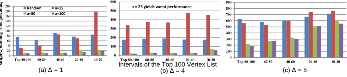
twitter-2010: (a) PageRank: Max = 3.0, Min = 0.5, GeoMean = 1.6; (b)Clique: Max = 48.3, Min = 4.1, GeoMean = 13.4; and (c) Community: Max = 7.5, Min = 1.4, GeoMean = 4.2. . . 32 2.4 GraphQ’s running time (in seconds) for answering PageRank queries over

twitter-2010 using different abstraction graphs: Random means no refinement is used and partitions are merged randomly; a = i means a partition is represented by i

abstract vertices. . . 34

3.1 A program and its expression graph: solid, horizontal edges represent assignments (A- and M- edges); dashed, vertical edges represent dereferences (D-edge); dotted, horizontal edges represent transitive edges labeled non-terminals. A4 indicates the allocation site at Line 4. . . 45 3.2 (a) An example graph, (b) its partitions, and (c) the in-memory representation

of edge lists. . . 51 3.3 Two representative bugs in the Linux kernel 4.4.0-rc5 that were missed by the

baseline checkers. . . 62 3.4 Percentages of added edges across supersteps. . . 66

4.1 A Triangle Counting example in RStream; highlighted in each table is its key column. For each table, only a small number of relevant tuples are shown. . . . 77 4.2 Triangle counting in RStream. . . 78

(13)

4.3 Major data structures. . . 82 4.4 API functions. . . 83 4.5 A graphical illustration of join on all columns; the streaming partitions #1 and

#2 contain vertices [0, 10] and [11, 25], respectively; suppose new key returns 2 (which is column C3). Structural info is not shown. . . 86

4.6 An FSM program; structural info is needed. . . 87 4.7 A graphical illustration of multiple producers, multiple consumers and reshuffling

buffers. . . 91 4.8 A graph and its canonical tuples of size 3. . . 93 4.9 Aggregation example of three isomorphic tuples. . . 94 4.10 FSM performance comparisons with different pattern sizes and supports over the

Patents graph. Tall red bars on the right of each group represent Arabesque failures. . . 100 4.11 (a) Comparisons between RStream (RS), BigDatalog (BD-n), and SociaLite (SL)

on TC and CC; (b) Closure comparison over CiteSeer. . . 102 4.12 RStream’s scalability (a), I/O throughput when running CC over UK (b), and

(14)

LIST OF TABLES

2.1 A summary of queries performed in the evaluation: reported are the names and forms of the queries, initial partition selection, priority of partition merging, whole-graph computation times in GraphChi for theuk-2005and thetwitter-2010 graphs, and the time for pre-processing them; ↑(↓) means the higher (lower) the better; each pre-processing time has two componentsa+b, wherearepresents the time for partitioning and AG construction, and b represents the time for initial (local) computation; “?” means the whole-graph computation cannot finish in 48 hours. . . 24 2.2 Our graph inputs: reported in each section are their names, types, numbers of

vertices, numbers of edges, numbers of initial partitions (IP), numbers of maxi-mum partitions allowed to be merged before out of budget (MP), and numbers of partitions increased at each step (δ, cf.line 13 in Figure 2.2). . . 25 2.3 GraphQ performance for answering PageRank queries over uk-2005; each section

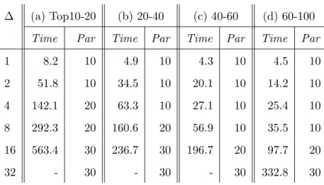
shows the performance of answering queries on pagerank values that belong to an interval in the top 100 vertex list; reported in each section are the number of entities requested to find (∆), the average query answering time in seconds (Time), and the number of partitions merged when a query is answered (Par). 28 2.4 GraphQ’s performance for answering Clique queries over twitter-2010; a “-” sign

means some queries in the group could not be answered. . . 29 2.5 GraphQ’s performance for answering Community queries over uk-2005; each

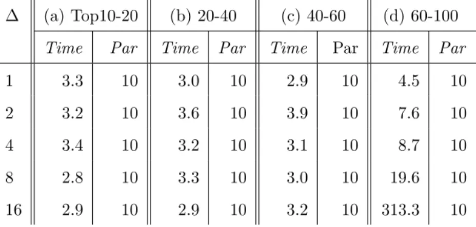
sec-tion reports the average time for finding communities whose sizes belong to dif-ferent intervals in the top 100 community list. . . 30 2.6 GraphQ’s performance for answering Path queries over twitter-2010. . . 30 2.7 GraphQ’s performance for answering Trianglequeries over uk-2005. . . 31

(15)

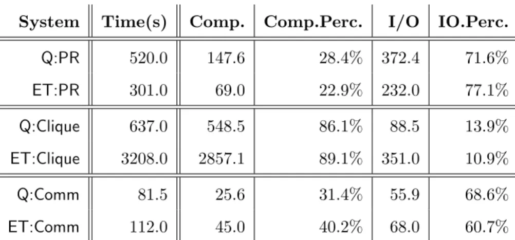
2.8 A breakdown of time on computation and I/O for GraphQ and GraphChi-ET for PageRank, Clique, and Comm; measurements were obtained by running the most difficult queries from Figure 2.3. . . 33

3.1 A subset of checkers used by [44] and [113] to find bugs in the Linux kernel, their target problems, their limitations, the potential ways to improve them using a sophisticated interprocedural analysis; the first six have been used by Chou et al. [53] and Palix et al. [113] to study Linux bugs; the last one was described in a recent paper by Brown et al. [44] to find potential NULL pointer deref-erences; positive/negative indicates whether the limitation can result in false positives/negatives. . . 38 3.2 Programs analyzed, their versions, numbers of lines of code, and numbers of

function inlines. . . 59 3.3 Checkers implemented, their numbers of bugs reported by the baseline checkers

(BL), and new bugs reported by our Graspan analyses (GR) on top of the BL checkers on the Linux kernel 4.4.0-r5; RE shows total numbers of bugs reported while FP shows numbers of false positives determined manually; to provide a reference of how bugs evolve over the last decade, we include an additional section

BL(2.6.1) with numbers of true bugs reported by the same checkers in 2011 on the kernel version 2.6.1 from [113]. UNTest is a new interprocedural checker we implemented to identify unnecessary NULL tests; ‘+’ means new problems found. 60 3.4 A breakdown of the new Linux bugs found by our analyses; in parentheses are

numbers of false positives. . . 63 3.5 Graspan performance: reported are the numbers of vertices and edges before (IS)

and after (PS) being processed by Graspan, Graspan’s pre-processing time (PT), numbers of supersteps taken (#SS), and total running time (T). . . 64

(16)

3.6 A comparison on the performance of Graspan, on-demand pointer analysis (ODA) [174] implemented in standard ways, as well as SociaLite [90] processing our program graphs in Datalog. The Graspan section shows a breakdown of the running times into computation time (CT), I/O time (I/O), and garbage collection time (GC); P and D represent pointer/alias analysis and dataflow analysis. OOM means out of memory. . . 65

4.1 Real world graphs. . . 96 4.2 Algorithms experimented. . . 96 4.3 Comparisons between RStream (RS), Arabesque (AR-n), ScaleMine (SM-n), and

DistGraph(DG-n) on four mining algorithms — triangle counting (TC), Clique (k-C), Motif Counting (k-M), and FSM (k-F) — over three graphs CiteSeer (CS), MiCo (MC), and Patents (PA); nrepresents the number of nodes the distributed systems use; k is the size of the structure to be mined; ‘-’ indicates execution failures. For FSM, four different support parameters (300, 500, 1K, and 5K) are used and explicitly shown in each 3-F row. Highlighted rows are the shortest times (in seconds). . . 98 4.4 FSM performance comparisons between RStream and GraMi over Patents and

Mico; time is measured in seconds. . . 101 4.5 The number of tuples (Tuples) generated for each phase execution, the size of

each tuple (TS), and the number of bytes (#MB) shuffled for 4-Motif over the Patents graph and 4-FSM, S=10K over the Mico graph. . . 104 4.6 Ratios between the final disk usage and original graph size (in the binary format). 105

(17)

ACKNOWLEDGMENTS

I am deeply grateful to my advisor, Professor Harry Guoqing Xu, who has spent a tremendous amount of effort providing continuous support and guidance through my Ph.D. studies. He is thoughtful and passionate. During the past six years, I have learned how to pursue my research interests, collaborate with others, overcome challenges, and build practical systems. My graduate career would have not been possible without his dedicated mentorship. I am so proud to join his research group and be one of his students.

I would like to thank Professor Jens Palsberg, Professor Miryung Kim and Professor Todd Millstein, for serving on my final defense committee. Their valuable comments have always strengthened my research.

I would like to thank my colleagues, Zhiqiang Zuo, Khanh Nguyen, Lu Fang, Yingyi Bu, Aftab Hussain, Cheng Cai, Bojun Wang, John Thorpe, Tim Nguyen, Christian Navasca for their great support.

This work would not have been possible without the amazing encouragement and support from my wife and my parents. I thank my wife Yamin for her love and support, for every day we have spent together, for her taking care of most of the family duties during my six years’ Ph.D. studies. I thank my daughter Annie for filling my life with love and happiness. I thank my parents Dequn and Gaixiang for their continuous support, for believing in me.

The material presented in this dissertation is based upon work supported by the Na-tional Science Foundation under the grants CCF-1054515, CCF-1117603, CNS-1321179, CNS-1319187, CCF-1349528, and CCF-1409829, and by the Office of Naval Research un-der grant N00014-14- 1-0549 and N00014-16-1-2913.

(18)

VITA

2018-2019 Graduate Research Assistant, Computer Science Department, UCLA

2013-2018 Graduate Research Assistant, Computer Science Department, UC Irvine

Jun 2009 Master of Science in Computer Science, Chinese Academy of Sciences, Bei-jing, China

Jun 2006 Bachelor of Science in Computer Science, Huazhong University of Science and Technology, Wuhan, China

PUBLICATIONS

Zhiqiang Zuo, John Thorpe, Yifei Wang, Qiuhong Pan, Shenming Lu, Kai Wang, Guoqing Harry Xu, Linzhang Wang, and Xuandong Li. Grapple: A Graph System for Static Finite-State Property Checking of Large-Scale System Code. InEuropean Conference on Computer Systems (EuroSys’19), Article No. 38, 2019.

Kai Wang, Zhiqiang Zuo, John Thorpe, Tien Quang Nguyen, and Guoqing Harry Xu. RStream: Marrying Relational Algebra with Streaming for Efficient Graph Mining on A Single Machine. In13th USENIX Symposium on Operating Systems Design and Implemen-tation (OSDI’18), pages 763-782, 2018.

Kai Wang, Aftab Hussain, Zhiqiang Zuo, Guoqing Xu, and Ardalan Amiri Sani. Graspan: A single-machine disk-based graph system for interprocedural static analyses of large-scale sys-tems code. In Proceedings of the Twenty-Second International Conference on Architectural Support for Programming Languages and Operating Systems (ASPLOS’17), pages 389–404,

(19)

2017.

Khanh Nguyen, Kai Wang, Yingyi Bu, Lu Fang, and Guoqing Xu. Understanding and Combating Memory Bloat in Managed Data-Intensive Systems. In ACM Transactions on Software Engineering and Methodology (TOSEM), 26, 4, Article 12 (January 2018).

Kai Wang, Guoqing Xu, Zhendong Su, and Yu David Liu. GraphQ: Graph query process-ing with abstraction refinement—programmable and budget-aware analytical queries over very large graphs on a single PC. In2015 USENIX Annual Technical Conference (USENIX ATC’15), pages 387–401, 2015.

Khanh Nguyen, Kai Wang, Yingyi Bu, Lu Fang, Jianfei Hu, and Guoqing Xu. Facade: A Compiler and Runtime for (Almost) Object-Bounded Big Data Applications. In Proceed-ings of the Twentieth International Conference on Architectural Support for Programming Languages and Operating Systems (ASPLOS’15), pages 675-690, 2015.

(20)

CHAPTER 1

Introduction

As graph data becomes ubiquitous in modern computing, developing systems to efficiently process large graphs has gained increasing popularity. Due to their importance in machine learning, web application and social media, graph analytical problems have been extensively studied in the past decade. Practical solutions have been implemented in a wide variety of graph systems [68, 52, 67, 72, 98, 88, 135, 105, 177, 126, 153, 173, 73, 125, 147, 176].

There are two major types of analytical problems over large graphs: graph computation and graph mining. Graph computation includes a set of problems that can be represented through liner algebra over an adjacency matrix based representation of the graph. As a typi-cal example of graph computation, PageRank [112] can be modeled as iterative sparse matrix and vector multiplications. Graph mining aims to discover complex structural patterns of a graph, for example, finding relationship patterns in social media network, detecting link spam in web data. As a typical example of graph mining, frequent sub-graph mining finds all sub-graphs with frequency above a user-defined threshold in a labeled input graph.

However, most of the existing systems for graph analytics are distributed frameworks, which suffer from one or more of the following drawbacks:

• In order to scale to large graphs, graph systems often need enterprise clusters with hundreds or even thousands of computation nodes. Many of the (current and future) users performing graph analytics will be domain experts with limited computer science background. It is much easier for them to host the system on their own machines rather than relying on a cluster, which involves tasks such as fault tolerance and cluster management they are not familiar with.

(21)

• Not all users have access to enterprise cluster in their daily development tasks. Even if they do, running a simple graph analytics on a relatively small graph does not seem to justify very well the cost of blocking hundreds or even thousands of machines for several hours.

• Load balancing in a distributed system is another major challenge. Algorithms such as frequent sub-graph mining have dynamic working sets. Their search space is often unknown in advance and it is thus hard to partition the graph and distribute the workload appropriately before the execution.

• Distributed graph systems commonly suffer from large startup and communication overhead. For small graphs, it is difficult for the startup/communication overhead to get amortized over the processing.

In this dissertation, we identify three categories of graph workloads for which single-machine systems can outperform distributed systems.

• Category 1: Analytical queries that do not need exact answers. For example, queries such as “find one path between LA and NYC whose length is less than 3,000 miles” have many usage scenariose.g., any path whose length is smaller than a thresh-old between two cities is acceptable for a navigation system. It appears that many of these analytical queries can be effectively computed by exploring only a small fraction of the graph, and traversing the complete graph is an overkill. If partial graphs are sufficient, we can answer analytical queries on one single PC so that the client can be satisfied without resorting to clusters.

• Category 2: Graph-based program analysis tasks that are widely used to find bugs in real-world software. Our key observation is that many interprocedural analyses can be formulated as a graph reachability problem [119, 139, 117, 129, 165]. Since program analysis is intended to assist developers to find bugs in their daily development tasks, their machines are the environments in which we would like our

(22)

system to run, so that developers can check their code on a regular basis without needing to access a cluster. Hence, disk-based graph system naturally becomes our choice.

• Category 3: Graph mining algorithms that are important for many informa-tion retrieval tasks. Mining workloads are memory-intensive because the amount of intermediate data for a typical mining algorithm grows exponentially with the size of the graph. By utilizing disk space available in modern machines, a disk-based system can satisfy the large storage requirement of mining algorithms.

The overarching goal of this dissertation is to build a set of efficient and scalable single-machine systems for important graph-analytical tasks. Our key insight is consistent with the recent trend on building single-machine graph computation systems [88, 126, 153, 148, 101, 173, 17, 177] — given the increasing accessibility of high-volume SSDs, a disk-based system can satisfy the large storage requirement of graph algorithms by utilizing disk space available in modern machines; yet it does not suffer from any startup and communication inefficiencies that are inherent in distributed computing. We make the following contributions:

• Contribution 1: A single-machine graph querying framework. We build GraphQ, a novel graph processing framework for analytical queries. The centerpiece of GraphQ is the novel idea of abstraction refinement, where the very large graph is rep-resented as multiple levels of abstractions, and a query is processed through iterative refinement across graph abstraction levels. As a result, GraphQ enjoys several distinc-tive traits unseen in existing graph processing systems: query processing is naturally

budget-aware, friendly for out-of-core processing when “Big Graphs” cannot entirely

fit into memory, and endowed with strong correctness properties on query answers. With GraphQ, a wide range of complex analytical queries over very large graphs can be answered with resources affordable to a single PC, which complies with the recent trend advocating single-machine-based Big Data processing.

(23)

memory capacity, only in several seconds to minutes. In contrast, GraphChi, a state-of-the-art graph processing system, takes hours to days to compute a whole-graph so-lution. An additional comparison with a modified version of GraphChi that terminates immediately when a query is answered shows that GraphQ is on average 1.6–13.4×

faster due to its ability to process partial graphs.

• Contribution 2: A single-machine graph system for interprocedural static analyses. We build Graspan, a single machine, disk-based parallel graph process-ing system tailored for interprocedural static analyses. Given a program graph and a grammar specification of an analysis, Graspan offers two major performance and scal-ability benefits: (1) the core computation of the analysis is automatically parallelized and (2) out-of-core support is exploited if the graph is too big to fit in memory. At the heart of Graspan is a parallel edge-pair (EP) centric computation model that, in each iteration, loads two partitions of edges into memory and “joins” their edge lists to produce a new edge list. Whenever the size of a partition exceeds a threshold value, its edges are repartitioned. Graspan supports both in-memory (for small programs) and out-of-core (for large programs) computation. Joining of two edge lists is fully parallelized, allowing multiple transitive edges to be simultaneously added.

We have implemented Graspan in both Java and C++. Graspan can be readily used as a “backend” analysis engine to enhance the existing static checkers such as BugFinder, PMD, or Coverity. We have performed a thorough evaluation of Graspan on three sys-tems programs including the Linux kernel, the PostgreSQL database, and the Apache httpd server. Our experiments show very promising results: (1) the two Graspan-based analyses scale easily to these systems, which have many millions of function inlines, with several hours processing time, while their traditional implementations crashed in the early stage; (2) in terms of LoC, the Graspan-based implementations of these analyses are an order-of-magnitude simpler than their traditional implementations; (3) using the results of these interprocedural analyses, the static checkers in [113] have uncovered a total of 85 potential bugs.

(24)

• Contribution 3: A single-machine graph mining framework. We build RStream,

a single-machine, out-of-core mining system that leverages disk support to store

in-termediate data. At its core are two innovations: (1) To enable easy programming of mining algorithms with and without statically-known structural patterns, we propose a novel programming model, referred to as GRAS, which adds relational algebra into gather-apply-scatter (GAS) model. Many mining algorithms, including FSM, Trian-gle and Motif Counting, or Clique, can all be easily developed with less than 80 lines of code under GRAS; and (2) We build a runtime engine that implements relational algebra efficiently with tuple streaming. Since the number of edges/updates is much larger than the number of vertices for a graph, edge streaming provides efficiency by se-quentially accessing edge data from disk (as edges are sese-quentially read but not stored in memory) and randomly accessing vertex data held in memory. Streaming essen-tially provides anefficient, locality-aware join implementation. RStream leverages this insight to implement relational operations.

A comparison between RStream and four state-of-the-art distributed mining/Datalog systems — Arabesque, ScaleMine, DistGraph, and BigDatalog — demonstrates that RStream outperforms all of them, running on a 10-node cluster,e.g.by at least a factor of 1.7×, and can process large graphs on an inexpensive machine.

Impact GraphQ proposed in this dissertation is the first graph processing system that can answer analytical queries over partial graphs. GraphQ is built on a key insight that many interesting graph properties — such as finding cliques of a certain size, or finding vertices with a certain page rank — can be effectively computed by exploring only a small fraction of the graph, and traversing the complete graph is an overkill. With GraphQ, a wide range of complex analytical queries over very large graphs can be answered with resources affordable to a single PC. We hope that GraphQ will open up new possibilities to scale up Big Graph processing with small amounts of resources.

(25)

and leverage novel graph processing techniques to solve this traditional programming lan-guage problem. RStream uses an edge-pair centric computation model to computedynamic

transitive closures on very large program graphs. An evaluation of these static analyses on

large codebases such as Linux shows that their Graspan implementations scale to millions of lines of code and are much simpler than their original implementations. Moreover, we show that these analyses can be used to augment the existing checkers. We hope that our work will open up a new direction for scaling various sophisticated static program analyses (e.g., symbolic execution, theorem proving, etc.) to large systems.

RStream is the first single-machine, out-of-core graph mining system. RStream employs a new GRAS programming model that uses a combination of GAS and relational algebra to support a wide variety of mining algorithms. At the low level, RStream leverages tuple streaming to efficiently implement relational operations. Our experimental results demon-strate that RStream can be more efficient than state-of-the-art distributed mining systems. We hope that these promising results will encourage future work that builds disk-based systems to scale expensive mining algorithms.

Organization We propose GraphQ, a single-machine scalable querying framework for very large graphs in Chapter 2. Chapter 3 presents the design and implement of Graspan, a single-machine graph system tailored for interprocedural static analyses. Chapter 4 proposes RStream, a single-machine, out-of-core graph mining system that leverages disk support to store intermediate data. Related work is discussed in Chapter 5. Chapter 6 concludes the dissertation and presents future work.

(26)

CHAPTER 2

GraphQ: Graph Query Processing with Abstraction

Refinement

Developing scalable systems for efficient processing of very large graphs is a key challenge faced by Big Data developers and researchers. Given a graph analytical task expressed as a set of user-defined functions (UDF), existing processing systems compute acomplete solution

over the input graph. Despite much progress, computing a complete solution is still time-consuming. For example, using a 32-node cluster, it takes Preglix [45], a state-of-the-art graph processing system, more than 2,500 seconds to compute a complete solution (i.e., all communities in the input graph) over a 70GB webgraph for a simple community detection algorithm.

While necessary in many cases, the computation of complete solutions — and the over-head of maintaining them — seems an overkill for many real-world applications. For example, queries such as “find one path between LA and NYC whose length is≤3,000 miles” or “find 10 programmer communities in Southern California whose sizes are≥1000” have many real-world usage scenarios e.g., any path whose length is smaller than a threshold between two cities is acceptable for a navigation system. Unlike database queries that can be answered by filtering records, these queries need (iterative) computations over graph vertices and edges. In this chapter, we refer to such queries as analytical queries. Furthermore, it appears that many of them can be answered by exploring only a small fraction of the input graph — if a solution can be found in a subgraph of the input graph, why do we have to exhaustively traverse the entire graph?

(27)

real-world applications that need analytical queries, can we have a ground-up redesign of graph processing systems — from the programming model to the runtime engine — that can facilitate query answering overpartial graphs, so that a client application can quickly obtain satisfactory results? If partial graphs are sufficient, can we answer analytical queries on one single PC so that the client can be satisfied without resorting to clusters?

We propose GraphQ, a novel graph processing framework for analytical queries. In GraphQ, an analytical query has the form “find n entities from the graph with a given

quantitative property”, which is general enough to express a large class of queries, such as

page rank, single source shortest path, community detection, connected components,etc.At its core, GraphQ features two interconnected innovations:

• A simple yet expressive partition-check-refine programming model that naturally sup-ports programmable analytical queries processed throughincremental accesses to graph data

• A novel abstraction refinement algorithm to support efficient query processing, fun-damentally decoupling the resource usage for graph processing from the (potentially massive) size of the graph

From the perspective of a GraphQ user, the very large input graph can be divided into

partitions. How partitions are defined is programmable, and each partition on the high level

can be viewed as a subgraph that GraphQ queries operate on. Query answering in GraphQ follows a repeated lock-stepcheck-refine procedure, until either the query is answered or the budget is exhausted.

In particular, (1) thecheck phase aims to answer the query over each individual partition without considering inter-partition edges connecting these partitions. A query is successfully answered if acheck predicate returns true; (2) if not, a refine process is triggered to identify a set of inter-partition edges to add back to the graph. These recovered edges will lead to a broader scope of partitions to assist query answering, and the execution loops back to step (1). Both the check procedure (determining whether the query is answered) and the

(28)

refine procedure (determining what new inter-partition edges to include) are programmable, leading to a programming model suitable for defining complex analytical queries with sig-nificant in-graph computations.

Key to finding the most profitable inter-partition edges to add in each step is a novel

abstraction refinement algorithm at the core of its query processing engine. Conceptually,

the “Big Graph” under GraphQ is summarized into an abstraction graph, which can be intuitively viewed as a “summarization overlay” on top of the complete concrete graph (CG). The abstraction graph serves as a compact “navigation map” to guide the query processing algorithm to find profitable partitions for refinement.

Usage Scenarios We envision that GraphQ can be used in a variety of real-world data analytical applications. Example applications include:

• Target marketing: GraphQ can help a business quickly find a target group of customers

with given properties;

• Navigation: GraphQ can help navigation systems quickly find paths with acceptable

lengths

• Memory-constrained data analytics: GraphQ can provide good-enough answers for

analytical applications with memory constraints

2.1

Overview and Programming Model

Background Common to graph processing systems, the graph operated by GraphQ can be mathematically viewed as a directed (sparse) graph,G= (V,E). A value is associated with each vertex v ∈V, indicating an application-specific property of the vertex. For simplicity, we assume vertex values are labeled from 1 to |V|. Given an edge e of the form u → v in the graph, e is referred to as vertex v’s in-edge and as vertex u’s out-edge. The developer specifies an update(v) function, which can access the values of a vertex and its neighboring

(29)

vertices. These values are fed into a function f that computes a new value for the vertex. The goal of the computation is to “iterate around” vertices to update their values until a global “fixed-point” is reached. This vertex-centric model is widely used in graph processing systems, such as Pregel [102], Pregelix [45], and GraphLab [99].

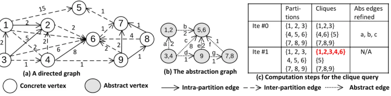
Figure 2.1 shows a simple directed graph that we will use as a running example throughout this chapter. For each GraphQ query, the user first needs to find a related base application

that performs whole-graph vertex-centric computation. This is not difficult, since many of these algorithms are readily available. In our example, the base application is Maximal Clique, and the query aims to find a clique whose size is no less than 5 (i.e. goal) over the input graph.

Parti- tions

Cliques Abs edges refined Ite #0 {1, 2, 3} {4, 5, 6} {7, 8, 9} {1,2,3} {4,6} {5} {7,8,9} a, b, c Ite #1 {1, 2, 3, 4, 5, 6} {7, 8, 9} {1,2,3,4,6} {5} {7,8,9} N/A

(c) Computation steps for the clique query 1,2 3,4 5,6 7,8 9 a b c d e f g 2 1 2 ₈ 1 ₁ 2

(b) The abstraction graph

1 3 2 4 5 6 7 8 9 15 2 1 2 5 2 2 1 8 1 1 1 1 2 4 6 2 2

(a) A directed graph

Concrete vertex Abstract vertex _{Intra-partition edge} _{Inter-partition edge} _{Abstract edge}

Figure 2.1: An example graph, its abstraction graph, and the computation steps for finding a clique whose size is ≥5. The answer of the query is highlighted.

GraphQ first divides the concrete graph in Figure 2.1 (a) into threepartitions —{1, 2, 3},

{4, 5, 6}, and {7, 8, 9}— a “pre-processing” step that only needs to be performed once for each graph. When the query is submitted, the goal of GraphQ is to use anabstraction graph

to guide the selection of partitions to be merged, hoping that the query can be answered by merging only a very small number of partitions. Initially, inter-partition edges (shown as arrows with dashed lines) are disabled; they will be gradually recovered.

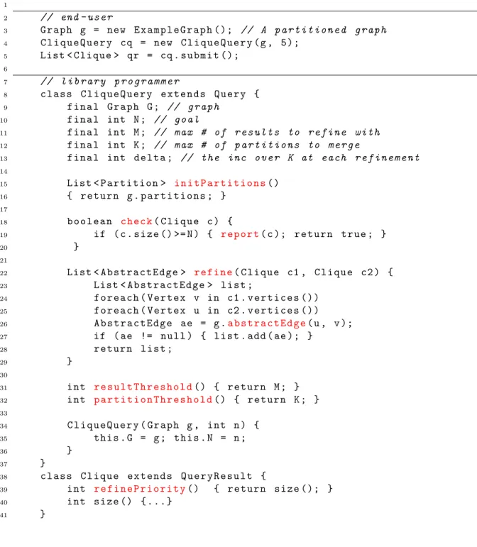
Programming Model A sample program for answering the clique query can be found in Figure 2.2. Overall, GraphQ is endowed with an expressive 2-tier programming model to

(30)

1 2 // end - u s e r 3 G r a p h g = new E x a m p l e G r a p h (); // A p a r t i t i o n e d g r a p h 4 C l i q u e Q u e r y cq = new C l i q u e Q u e r y ( g , 5); 5 List < Clique > qr = cq . s u b m i t (); 6 7 // l i b r a r y p r o g r a m m e r 8 c l a s s C l i q u e Q u e r y e x t e n d s Q u e r y { 9 f i n a l G r a p h G ; // g r a p h 10 f i n a l int N ; // g o a l 11 f i n a l int M ; // max # of r e s u l t s to r e f i n e w i t h 12 f i n a l int K ; // max # of p a r t i t i o n s to m e r g e

13 f i n a l int d e l t a ; // the inc o v e r K at e a c h r e f i n e m e n t

14 15 List < P a r t i t i o n > i n i t P a r t i t i o n s() 16 { r e t u r n g . p a r t i t i o n s ; } 17 18 b o o l e a n c h e c k( C l i q u e c ) { 19 if ( c . s i z e () >= N ) { r e p o r t( c ); r e t u r n t r u e ; } 20 } 21 22 List < A b s t r a c t E d g e > r e f i n e( C l i q u e c1 , C l i q u e c2 ) { 23 List < A b s t r a c t E d g e > l i s t ; 24 f o r e a c h ( V e r t e x v in c1 . v e r t i c e s ()) 25 f o r e a c h ( V e r t e x u in c2 . v e r t i c e s ()) 26 A b s t r a c t E d g e ae = g .a b s t r a c t E d g e( u , v ); 27 if ( ae != n u l l ) { l i s t . add ( ae ); } 28 r e t u r n l i s t ; 29 } 30 31 int r e s u l t T h r e s h o l d() { r e t u r n M ; } 32 int p a r t i t i o n T h r e s h o l d() { r e t u r n K ; } 33 34 C l i q u e Q u e r y ( G r a p h g , int n ) { 35 t h i s . G = g ; t h i s . N = n ; 36 } 37 } 38 c l a s s C l i q u e e x t e n d s Q u e r y R e s u l t { 39 int r e f i n e P r i o r i t y() { r e t u r n s i z e (); } 40 int s i z e () { . . . } 41 }

(31)

balance simplicity and programmability:

• First, GraphQ end users only need to write 2-3 lines of code to submit a query. For example, the end user writes lines 2-5, submitting a CliqueQuery to look for Clique

instances whose size is no fewer than 5 over the ExampleGraph.

• Second, GraphQ library programmers define how a query can be answered through a flexible programming model that fully supports in-graph computation. In the example, the clique query is defined between lines 7-40, by extending theQueryandQueryResult

classes in our library.

We expect regular GraphQ users — those who only care aboutwhat to query but nothow

to query it — to program only the first tier (between lines 2-5). The appeal of the GraphQ programming model lies in its flexibility. On one hand, the simplicity of the GraphQ first-tier interface is on par with query languages for similar purposes (such as SQL). On the other hand, for programmers concerned with graph processing efficiency, GraphQ provides opportunities for full-fledged programming “under the hood” at the second tier.

Partitions Given a very large graph, one can specify how it is partitioned using GraphQ parameters. A partition is both a logical and a physical concept. Logically, a partition is a subgraph (connected component) of the concrete graph. Physically, it is often aligned with the physical storage unit of data, such as a disk file. In our formulation where the graph vertices are labeled with numbers from 1 to |V|, we select partitions as containing vertices with continuous label numbers, and edges connecting those vertices in the concrete graph. Beyond this mathematical formulation is an intuitive goal: if we use labels 1 to|V|to mimic the physical sequence of vertex storage, the partitions should be created to be as aligned with physical storage as possible. Thanks to this design, loading a partition is very efficient due to sequential disk accesses with strong locality.

When a query is defined — such as CliqueQuery — the programmer first decides what partitions should be initially considered to compute local solutions (e.g. cliques). This is

(32)

supported by overriding the initPartitions method of the Query class, as in line 16. In our example, this method selects all partitions because we have no knowledge of whether and what cliques exist in each partition initially. GraphQ loads one partition into memory at a time and performs vertex-centric computation on the partition to compute local cliques independently of other partitions.

Observe that this does not contradict with our early discussion of incremental graph data processing: at the local computation phase, all partition-based computations are independent of each other. Therefore, when the data for one partition is loaded, the data for previously loaded partitions can be written back to disk, and at this phase GraphQ does not need to hold data in memory for more than one partition. Overall, this phase is very efficient because all inter-partition edges are ignored and there are only a very small number of random disk accesses.

Abstraction Graph The abstraction graph (AG) summarizes the concrete graph. Each

abstract vertex in the AG abstracts a set of concrete vertices and eachabstract edge connects

two abstract vertices. An abstract edge can have anabstract weight that abstracts the weights of the actual edges it represents.

To see the motivation behind the design of AG, observe that inter-partition edges can scatter across the partitions (i.e., disk files) they connect, and knowing whether a concrete edge exists between two partitions requires loading both partitions into memory and a linear scan of them, a potentially costly step with a large number of disk accesses. As a “summa-rization” of the concrete graph, the AG is much smaller in size and can be always held in memory.

GraphQ first checks the existence of an abstract edge on the AG: the non-existence of an abstract edge between two abstract vertices ¯u and ¯v guarantees the non-existence of a concrete edge between any pair of concrete vertices (u,v) abstracted by ¯uand ¯v; hence, we can safely skip the check of concrete edges. On the other hand, the existence of an abstract edge does not necessarily imply the existence of a concrete edge, and hence, the abstract

(33)

edge needs to be refined to recover the concrete edges it represents.

The granularity of the AG is a design issue to be determined by the user. At one extreme, each partition can be an abstract vertex in the AG. This very coarse-grained abstraction may not be precise enough for GraphQ to quickly eliminate infeasible concrete edges. At the other extreme, a very fine-grained AG may take much space and the computation over the AG (such as a lookup) may take time. Since the AG is always in memory to provide quick guidance, a rule of thumb is to allow the abstraction granularity (i.e., the number of concrete vertices represented by one abstract vertex) to be proportional to the memory capacity.

Using parameters, the user can specify the ratio between the size of the AG and the main memory — the more memory a system has, the larger AG will be constructed by GraphQ to provide more precise guidance. Figure 2.1 (b) shows the AG for the concrete graph in Figure 2.1 (a). The GraphQ runtime uses the simple interval domain [55] to abstract concrete vertices — each abstract vertex represents two concrete vertices that have consecutive labels. This simple design turns out to be friendly for performance as well: each abstract edge represents a set of concrete edges stored together in the partition file; since refining an abstract edge needs to load its corresponding concrete edges, storing/loading these edges together maximizes sequential disk accesses and data locality. A detailed explanation of the storage structure can be found in Section 2.3.

An alternative route we decide not to pursue is to provide the user full programmability to construct their own AGs. The issue at concern iscorrectness. Our design of the abstraction graph is built upon the principled idea of abstraction refinement, with correctness guarantees (Section 2.2). The correctness is hinged upon that the AG is indeed a “sound” abstraction of the concrete graph. We rely on the GraphQ runtime to maintain this notion of sound abstraction.

Abstraction Refinement At the end of each local computation (i.e., over a partition), GraphQ invokes the check method of the Query object. The method returns true if the query can be answered, and the result is reported through thereport method (see line 19).

(34)

Query processing terminates. If all local computations are complete and allcheckinvocations returnfalse, GraphQ tries to merge partitions to provide a larger scope for query answering. Recall that in our initial partition definition, all inter-partition edges have been ignored. The crucial challenge of partition merging thus becomes recovering the inter-partition edges, a process we call abstraction refinement.

In GraphQ, the refinement process is guided by the QueryResult — Clique in our example — from local computations. The key insight is that the results so far should offer clues on which partitions should be merged at a higher priority. The “priority” here can be customized by programmers through overriding the refinePriority method of class

QueryResult. In the clique query example here, the programmer uses the size of the clique as the metric for priority (see line 39). Intuitively, merging partitions where larger cliques have been discovered is more likely to reach the goal of finding a clique of a certain size.

GraphQ next selectsM (returned byresultThresholdin line 31) results with the highest priorities (i.e. largest cliques) for pairwise inspection. For each pair of cliques resulting from different partitions, the refinemethod (line 22) is invoked to verify if there is any potential for the two input cliques to combine into a larger clique. refine returns a list of abstract edges that should be refined. The implementation of refine is provided by programmers, typically involving the consultation of the AG. In our example, the method returns a list of candidate abstract edges whose corresponding concrete edges may potentially connect vertices from the two existing cliques (in two partitions) in order to form a larger clique.

Based on the returned abstract edges, GraphQ consults the AG to find the concrete edges these abstract edges represent. GraphQ then merges the partitions in which these concrete edges are located. To avoid a large number of partitions to be merged at a time — that would require the data associated all partitions to be loaded into memory at the same time — programmers can set a threshold specified by partitionThresold, in line 32. GraphQ adopts an iterative merging process: in each pass, merging only happens when the refinement leads to the merging of no more than K (returned by partitionThresold) partitions. If the merged partitions cannot answer the queries, GraphQ increasesK byδ (line 13) at each

(35)

subsequent pass to explore more partitions. This design enables GraphQ to gradually use more memory as the query processing progresses.

GraphQ terminates query processing in one of the 3 scenarios: (1) the check method returns true, in which case the query is answered; (2) all partitions are merged in one, and the check method still returns false — a situation in which this query is impossible to answer; and (3) a (memory) budget runs out, in which case GraphQ returns the best

QueryResults that have been found so far. We will rigorously define this notion in Section 2.2.

Example Figure 2.1 (c) shows the GraphQ computational steps for answering the clique query. The three columns in the table show the partitions considered in the beginning of each iteration, the local maximal cliques identified, and the abstract edges selected by GraphQ to refine at the end of the iteration, respectively. Before iteration #0, the user selects all the three partitions via initPartitions. The vertex-centric computation of these partitions identifies four local cliques {1, 2, 3},{4, 6},{5}, and {7, 8, 9}.

Since the check function cannot find a clique whose size is ≥ 5, GraphQ ranks the four local cliques based on their sizes (by calling refinePriority) and invokesrefine five times with the following clique pairs: ({1, 2, 3}, {7, 8, 9}), ({1, 2, 3}, {4, 6}), ({4, 6}, and {7, 8, 9}), ({5},{1, 2, 3}), ({5},{7, 8, 9}). For instance, for input ({1, 2, 3},{7, 8, 9}), no abstract edge exists on the AG that connects any vertex in the first clique with any vertex in the second. Hence, refine returns an empty list.

For input ({1, 2, 3}, {4, 6}), however, GraphQ detects that there is an abstract edge between every abstract vertex that represents {1, 2, 3} and every abstract vertex that rep-resents {4, 6}. The abstract edges connecting these two cliques (i.e., a, b, and c) are then added into list listand returned.

After checking all pairs of cliques, GraphQ obtains 6 lists of abstract edges, among which five span two partitions and one spans three. Suppose K is 2 at this moment. The one spanning three partitions is discarded. For the remaining five lists, (a, b, c) is the first list

(36)

returned by refine (on input ({1, 2, 3}, {4, 6})). These three abstract edges are selected and their refinement adds the following four concrete (inter-partition) edges back to the graph: 4→2, 3→4, 1→5, and 2→6. The second iteration repeats vertex-centric computation by considering a merged partition {1, 2, 4, 5, 6}. When the partition is processed, a new clique {1, 2, 3, 4, 6} is found. Function check finds that the clique answers the query; so it reports the clique and terminates the process.

Programmability Discussions In addition to answering queries with user-specified goals, our programming model can also support aggregation queries (min, max, average,etc.). For example, to find the largest clique under a memory budget, only minor changes are needed to the CliqueQuery example. First, we can define a private field called max to the class. Second, we need to update the check method as follows:

if(c.size()>max)

{ max=c.size(); return false;}

The observation here is that check should always return false. GraphQ will continue the refinement until the (memory) budget runs out, and the result c aligns with our intu-ition of being “the largest Clique under the budget based on the user-specified refinement heuristics”, a flavor of the budget-aware query processing.

GraphQ can also support multiplicity of results, such as the top 30 largest cliques. This is just a variation of the example above. Instead of reporting a clique c, the CliqueQuery

should maintain a “top 30” list, and use it as the argument for report.

Trade-off Discussions It is clear that GraphQ provides several trade-offs that the user can explore to tune its performance. First, the memory size determines GraphQ’s answerability. A higher budget (i.e. more memory) will lead to (1) finding more entities with higher goals, or (2) finding the same number of entities with the same goals more quickly. Since GraphQ can be embedded in a data analytical application running on a PC, imposing a memory budget allows the application to perform intelligent resource management between GraphQ

(37)

an other parts of the system, obtaining satisfiable query answers while preventing GraphQ from draining the memory.

Another tradeoff is defined by abstraction granularity, that is, the ratio between the size of the AG and the memory size. The larger this ratio is, the more precise guidance the AG provides. On the other hand, holding a very large AG in memory could hurt performance by eclipsing the memory that could have been allocated for data loading and processing. Hence, achieving good performance dictates finding the sweetspot.

2.2

Abstraction-Guided Query Answering

This section formally presents our core idea of applying abstracting refinement to graph processing. In particular, we rigorously define GraphQ’s answerability.

Definition 2.2.1 (Graph Query). A user query is a 5-tuple (∆, φ, π, , g) that requests to find, in a directed graph G = (VG, EG), ∆ entities satisfying a pair of predicates hφ, πgi. Definition predicate φ∈Φ is a logical formula (_P(G)→_B) over the set of all G’s subgraphs that defines an entity,π ∈Πis a quantitative function (_P(G)→_R) over the set of subgraphs

satisfying φ, measuring the entity’s size, and is a numerical comparison operator (e.g., ≥

or =) that compares the output of π with a user-specified goal of the query g ∈_R.

This definition is applicable to a wide variety of user queries. For example, for the clique query discussed in Section 2.1, φ is the following predicate on the vertices and edges of a subgraph S ⊆G, defining a clique:

∀ v1, v2 ∈VS: ∃e∈ES: e= (v1, v2)∨e= (v2, v1),

while π is a simple function that returns the number of vertices|VS| in the subgraph. and

g are ≥ and 5, respectively. From this point on, we will refer to φ and π as the definition predicate and the size function, respectively.

Definition 2.2.2 (Monotonicity of the Size Function). A query (∆, φ, π, , g) is

(38)

P(G) :S2 ⊆S1∧φ(S1)∧φ(S2) =⇒ π(S1)π(S2).

While the user can specify an arbitrary size function π or goal g, π has to be monotone

in order for GraphQ to answer the query. More precisely, for any subgraphs S1 and S2 of

the input graphG, if S2 is a subgraph ofS1 and they both satisfy the definition predicateφ,

the relationship between their sizes π(S1) andπ(S2) isπ(S1)π(S2). For example, if S2 is a

clique with N vertices, andS1 is a supergraph ofS2 and also a clique,S1’s size must be≥N.

Monotonicity of the size function implies that once GraphQ finds a solution that satisfies a query at a certain point, the solution will always satisfy the query because GraphQ will only find better solutions in the forward execution. It also matches well with the underlying vertex-centric computation model that gradually propagates the information of a vertex to distant vertices (i.e., which has the same effect as considering increasingly large subgraphs).

Definition 2.2.3 (Partition). A partition P of graph G is a subgraph (VP, EP) of G such that vertices in VP have contiguous labels [i, i + |VP|], where i ∈I is the minimum integer

label a vertex in VP has and |VP| is the number of vertices of P. A partitioning of G

produces a set of partitions P1, P2, . . . Pk such that ∀j ∈ [1, k−1] : maxv∈V_Pjlabel(v) + 1 = minv∈V_Pj+1label(v). An edge e = (v1, v2) is an intra-partition edge if v1 and v2 are in the

same partition; otherwise, e is an inter-partition edge.

Logically, each partition is defined by a label range, and physically, it is a disk file containing the edges whose targets fall into the range. The physical structure of a partition will be discussed in Section 2.3.

Definition 2.2.4 (Abstraction Graph). An abstraction graph (V ,¯ E, α, γ¯ ) summarizes a

concrete graph (V, E) using abstraction relation α: V →V¯. The AG is a sound abstraction

of the concrete graph if ∀e = (v1, v2) ∈ E : ∃e¯ = ( ¯v1,v¯2) ∈ E¯ : ¯v1,v¯2 ∈ V¯ ∧(v1,v¯1) ∈

α∧(v2,v¯2)∈α. γ: V¯ →V is a concretization relation such that (¯v, v)∈γ iff (v,v¯)∈α.

α and γ form a monotone Galois connection [55] between G and AG (which are both posets). There are multiple ways to define the abstraction function α. In GraphQ,α is de-fined based on an interval domain [55]. Specifically, each abstract vertex ¯v has an associated

(39)

interval [i, j]; (v,¯v) ∈ α iff label(v) ∈ [i, j]. The primary goal is to make concrete edges whose target vertices have contiguous labels stay together in a partition file. To concretize an abstract edge, GraphQ will only needsequential accesses to a partition file, thereby maximiz-ing locality and refinement performance. Different abstract vertices have disjoint intervals. The length of the interval is determined by a user-specified percentage r and the maximum heap sizeM—the size of the AG cannot be greater thanr×M. The implementation details of the partitioning and the AG construction can be found in Section 2.3. Clearly, the AG constructed by the interval domain is a sound abstraction of the input graph.

Lemma 2.2.5 (Edge Feasibility). If no abstract edge exists from v¯1 to v¯2 on the AG, there must not exist a concrete edge fromv1 tov2 on the concrete graph such that (v1,v¯1)∈α and

(v2,v¯2)∈α.

The lemma can be easily proved by contradiction. It enables GraphQ to inspect the AG first to quickly skip over infeasible solutions.

Definition 2.2.6 (Abstraction Refinement). Given a subgraph S = (Vs, Es) of a concrete graph G= (V, E) and its AG = (V¯, E¯) ofG, an abstraction refinement vonS selects a set of abstract edgese¯∈E¯ and adds into Es all such concrete edgese thate∈E\Es : (¯e, e)∈α. An abstraction refinement of the form S vS0 produces a new subgraph S0 = (V_s0, E_s0), such that Vs = Vs0 and Es ⊆Es0. A refinement is an effective refinement ifEs ⊂Es0.

The concretization function is used to obtain concrete edges for a selected abstract edge. After an effective refinement, the resulting graph S0 becomes a (strict) supergraph of S, providing a larger scope for query answering.

Lemma 2.2.7 (Refinement Soundness). An entity satisfying the predicates (φ, πg) found

in a subgraph S is preserved by an abstraction refinement on S.

The lemma shows an important property of our analysis. Since our goal is to find ∆ entities, this property guarantees that the entities we find in previous iterations will stay as

(40)

we enlarge the scope. The lemma can be easily proved by considering Definition 2.2.2: since the size functionπ is monotone, if the predicate π(S)g holds in subgraph S, the predicate

π(S0)g must also hold in subgraph S0 that is a strict supergraph of S. BecauseS0 contains all vertices and edges ofS, the fact the definition predicate φ holds onS implies that φ also holds on S0 (i.e., φ(S) =⇒ φ(S0)).

Definition 2.2.8 (Essence of Query Answering). Given an initial subgraph S = (V, Es) composed of a set_P of disjoint partitions ((V1, E1),. . ., (Vj, Ej)) such thatV = V1∪. . .∪Vj andEs = E1∪. . .∪Ej, as well as an AG = (V¯, E¯), answering a query (∆, φ, π, , g) aims to find a refinement chain S v∗ _S00 _{such that there exist at least} _∆ _{distinct entities in} _S00_,

each of which satisfies both φ and πg.

In the worst case, S00 becomes G and graph answering has (at least) the same cost as computing a whole-graph solution. Each refinement step bridges multiple partitions. Sup-pose we have a partition graph (PG) for Gwhere each partition is a vertex. The refinement chain starts with a PG without edges (i.e., each partition is a connected component), and gradually adds edges and reduces the number of connected components. Suppose PGS is

the PG for a subgraphS,ρis a function that takes aPG as input and returns the maximum number of partitions in a connected component of thePG, and each initial partition has the (same) size η. We have the following definition:

Definition 2.2.9 (Budget-Aware Query Answering). Answering a query under a memory

budget M aims to find a refinement chain S v∗ _S00 _{such that}_∀₍_S

1 vS2)∈ v∗: η×ρ(PGS2)

≤M.

In other words, the number of (initial) partitions connected by each refinement step must not exceed a threshold t such that t×η ≥M. Otherwise, the next iteration would not have enough memory to load and process these t partitions.

Theorem 2.2.10 (Soundness of Query Answering). GraphQ either returns correct solutions or does not return any solution if the vertex-centric computation is correctly implemented.

(41)

Limitations Despite its practical usefulness, GraphQ can only answer queries whose vertex update functions are monotonic, while many real-world problems may not conform to this property. For example, for machine learning algorithms that perform probability propagation on edges (e.g., belief propagation and the coupled EM (CoEM)), the probability in a vertex may fluctuate during the computation, preventing the user from formulating a probability problem as GraphQ queries.

2.3

Design and Implementation

We have implemented GraphQ based on GraphChi [88], a high-performance single-machine graph processing system. GraphChi has both C++ and Java versions; GraphQ is imple-mented on top of its Java version to provide an easy way for the user to write UDFs. Our implementation has an approximate of 5K lines of code and is available for download on BitBucket. The pre-processing step splits the graph file into a set of small files with the same format, each representing a partition (i.e., a vertex interval). We modify the shard

construction algorithm in GraphChi to partition the graph. Similarly to a shard in [88], each partition file contains all in-edges of the vertices that logically belong to the parti-tion; hence, edges stored in a partition file whose sources do not belong to the partition are inter-partition edges.

The AG is constructed when the graph is partitioned. To allow concrete edges (i.e., lines in each text file) represented by the same abstract edge to be physically located together, we first sort all edges in a partition based on the labels of their source vertices — it moves together edges from contiguous vertices. Next, for each abstract vertex (i.e., an interval), we sort edges that come from this interval based on the labels of their target vertices — now the concrete edges represented by the same abstract edge are restructured to stay in a contiguous block of the file. This is a very important handling and will allow efficient disk accesses, provided that large graph processing is often I/O dominated.

(42)

physically in the partition file containing the vertex range [1024, 1268]. The first sort moves all edges coming from [40, 80] together. However, among these edges, those going to [1024, 1268] and those not are mixed. The second sort moves them around based on their target vertices, and thus, edges going to contiguous vertices are stored contiguously. Although the interval length used in the abstraction is statically fixed (i.e., defined as a user parameter), we do not allow an abstract vertex to represent concrete vertices spanning two partitions — we adjust the abstraction interval if the number of the last set of vertices in a partition is smaller than the fixed interval size.

Each abstract edge consists of the starting and ending positions of the concrete edges it represents (including the partition ID and the line offsets), as well as various summaries of these edges, such as the number of edges, and the minimum and maximum of their weights. The AG is saved as a disk file after the construction. It will be loaded into memory upon query answering. When an (initial or merged) partition is processed, we modify the parallel sliding window algorithm in GraphChi to load the entire partition into memory. In GraphChi, a memory shard is a partition being processed whilesliding shards are partitions containing out-edges for the vertices in the memory shard. Since inter-partition edges are ignored, GraphQ eliminates sliding shards and treats each partition p as a memory shard. The number of random disk accesses at each step thus equals the number of initial partitions contained in p.

The loaded data may include both enabled and disabled edges; the disabled edges are ig-nored during processing. Initially, all inter-partition edges are disabled. Refining an abstract edge loads the partitions to be merged and enables the inter-partition edges it represents before starting the computation. We treat the refinement process as an evolving graph, and modify the incremental algorithm in GraphChi to only compute and propagate values from the newly added edges.

A user-specified ratio r is used to control the size of the AG. Ideally, we do not want the size of the AG to exceed r× the memory size. However, this makes it very difficult to select the interval size (i.e. abstraction granularity) before doing partitioning, because

(43)

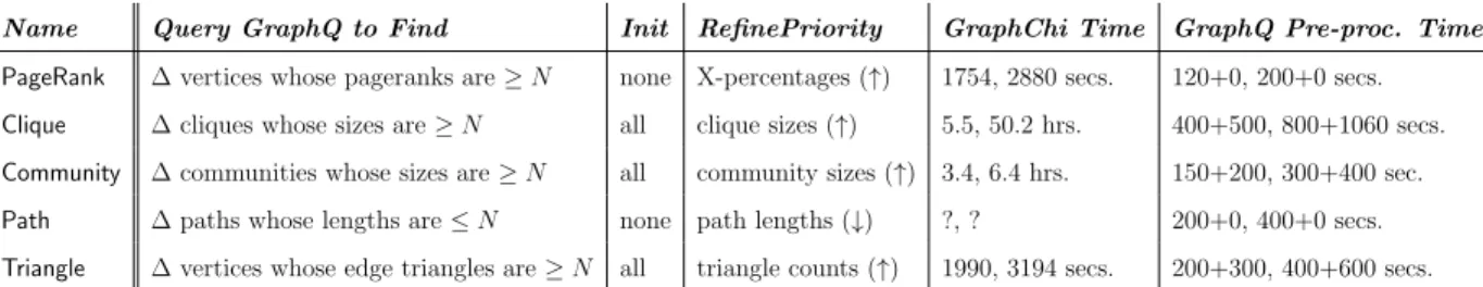
Name Query GraphQ to Find Init RefinePriority GraphChi Time GraphQ Pre-proc. Time

PageRank ∆ vertices whose pageranks are≥N none X-percentages (↑) 1754, 2880 secs. 120+0, 200+0 secs. Clique ∆ cliques whose sizes are≥N all clique sizes (↑) 5.5, 50.2 hrs. 400+500, 800+1060 secs. Community ∆ communities whose sizes are≥N all community sizes (↑) 3.4, 6.4 hrs. 150+200, 300+400 sec. Path ∆ paths whose lengths are≤N none path lengths (↓) ?, ? 200+0, 400+0 secs. Triangle ∆ vertices whose edge triangles are≥N all triangle counts (↑) 1990, 3194 secs. 200+300, 400+600 secs.

Table 2.1: A summary of queries performed in the evaluation: reported are the names and forms of the queries, initial partition selection, priority of partition merging, whole-graph computation times in GraphChi for theuk-2005and thetwitter-2010graphs, and the time for pre-processing them;↑(↓) means the higher (lower) the better; each pre-processing time has two componentsa+b, wherearepresents the time for partitioning and AG construction, and

brepresents the time for initial (local) computation; “?” means the whole-graph computation cannot finish in 48 hours.

the size of the AG is related to its number of edges and it is unclear how this number is related to the interval size before scanning the whole graph. To solve the problem, we use the following formula to calculate the interval size i: i = size_M×r(G), under a rough estimation that if the number of vertices is reduced byitimes, the number of edges (and thus the size of the graph) is also reduced byi times. In practice, the size of the AG built using i is always close to M×r, although it often exceeds the threshold.

2.4

Queries and Methodology

We have implemented UDFs for five common graph algorithms shown in Table 2.1. The pre-processing time is a one-time cost, which does not contribute to the actual query an-swering time. ForPageRankand Path, GraphQ does not need to compute local results; what partitions to be merged can be determined simply based on the structure of each partition. We experimented GraphQ with a variety of graphs. This section reports our results with the two largest graphs, shown in Table 2.2. Since the focus of this work is not to improve the whole-graph computation, we have not run other distributed platforms.

(44)

Name Type |V| |E| #IP #MP δ

uk-2005[38] webgraph 39M 0.75B 50 30 10

twitter-2010 [87] social network 42M 1.5B 100 50 10

Table 2.2: Our graph inputs: reported in each section are their names, types, numbers of vertices, numbers of edges, numbers of initial partitions (IP), numbers of maximum partitions allowed to be merged before out of budget (MP), and numbers of partitions increased at each step (δ, cf.line 13 in Figure 2.2).

PageRank Answering PageRank queries is based on the whole-graph PageRank algorithm used widely to rank pages in a webgraph. The algorithm is not strictly monotone, because vertices with few incoming edges would give out more than they gain in the beginning and thus their pageranks values would drop in the first few iterations. However, after a short “warm-up” phase, popular pages would soon get their values back and their pageranks would continue to grow until the convergence is reached. To get meaningful pagerank values to query upon, we focus on the top 100 vertices reported by GraphChi (among many million vertices in a graph). Their pageranks are very high and these vertices represent the pages that a user is interested in and wants to find from the graph.

Focusing on the most popular vertices also allows us to bypass the non-monotonic com-putation problem—since the goals are very high, it is only possible to answer a query during monotonic phase (after the non-monotonic warm-up finishes). The refinement logic we im-plemented favors the merging of partitions that can lead to a larger X-percentage. The X-percentage of a partition is defined as the percentage of the outgoing edges of the vertex with the largest degree that stay in the partition. It is a metric that measures the complete-ness of the edges for the most popular vertex in the partition. The higher the X-percentage is, the quicker it is for the pagerank computation to reach a high value and thus the easier for GraphQ to find popular vertices. PageRank does not need a local phase—from the AG, we directly identify a list of partitions whose merging may yield a large X-percentage.

(45)

vertex in the graph. Since the input is a directed graph, a set of vertices forms a clique if for each pair of vertices u and v, there are two edges between them going both directions. GraphChi does not support variable-size edge and vertex data, and hence, we used 10 as the upper-bound for the size of a clique we can find. In other words, we associated with each edge and vertex a 44-byte buffer (i.e., 10 vertices take 40 bytes and used an additional 4-byte space in the beginning to save the actual length). Due to the large amount of data swapped between memory and disk, the whole-graph computation over twitter-2010 took more than 2 days.

Path is based on the SSSP algorithm and aims to find paths with acceptable length between a given source and destination. Similarly to Clique, we associated a (fixed-length) buffer with each edge/vertex to store the shortest path for the edge/vertex. Since none of our input graphs have edge weights, we assigned each edge a random weight between 1 and 5. However, the whole-graph computation could not finish processing these graphs in 2 days. To generate reasonable queries for GraphQ, we sampled each graph to get a smaller graph (that is 1/5 of the original graph) and ran the whole-graph SSSP algorithm to obtain the shortest paths between a specified vertex S (randomly chosen) and all other vertices in the sample graph. If there exists a path between S and another vertex v in the small graph, a path must also exist in the original graph. The SSSP computation over even the small graphs took a few hours.

Community is based on a community detection algorithm in which a vertex choos