A novel image compression algorithm for high resolution 3D reconstruction

A novel image compression algorithm for high resolution

3D reconstruction

SIDDEQ, M. M. and RODRIGUES, Marcos

<http://orcid.org/0000-0002-6083-1303>

Available from Sheffield Hallam University Research Archive (SHURA) at:

http://shura.shu.ac.uk/7940/

This document is the author deposited version. You are advised to consult the

publisher's version if you wish to cite from it.

Published version

SIDDEQ, M. M. and RODRIGUES, Marcos (2014). A novel image compression

algorithm for high resolution 3D reconstruction. 3D research, 5 (7), 17 pages.

Copyright and re-use policy

See http://shura.shu.ac.uk/information.html

3 D R E X P R E S S

A Novel Image Compression Algorithm for High Resolution

3D Reconstruction

M. M. Siddeq•M. A. Rodrigues

Received: 12 November 2013 / Revised: 12 January 2014 / Accepted: 25 February 2014 The Author(s) 2014. This article is published with open access at Springerlink.com

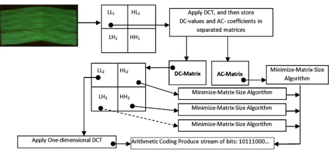
Abstract This research presents a novel algorithm to compress high-resolution images for accurate struc-tured light 3D reconstruction. Strucstruc-tured light images contain a pattern of light and shadows projected on the surface of the object, which are captured by the sensor at very high resolutions. Our algorithm is concerned with compressing such images to a high degree with minimum loss without adversely affecting 3D recon-struction. The Compression Algorithm starts with a single level discrete wavelet transform (DWT) for decomposing an image into four bands. The sub-band LL is transformed by DCT yielding a DC-matrix and an AC-matrix. The Minimize-Matrix-Size Algo-rithm is used to compress the AC-matrix while a DWT is applied again to the DC-matrix resulting in LL2,

HL2, LH2and HH2sub-bands. The LL2sub-band is

transformed by DCT, while the Minimize-Matrix-Size Algorithm is applied to the other sub-bands. The proposed algorithm has been tested with images of different sizes within a 3D reconstruction scenario. The algorithm is demonstrated to be more effective than JPEG2000 and JPEG concerning higher com-pression rates with equivalent perceived quality and

the ability to more accurately reconstruct the 3D models.

Keywords DWTDCT

Minimize-Matrix-SizeLSS-Algorithm3D reconstruction

1 Introduction

The researches in compression techniques has stemmed from the ever-increasing need for efficient data transmission, storage and utilization of hardware resources. Uncompressed image data require consid-erable storage capacity and transmission bandwidth. Despite rapid progresses in mass storage density, processor speeds and digital communication system performance demand for data storage capacity and data transmission bandwidth continues to outstrip the capabilities of available technologies [2]. The recent growth of data intensive multimedia based applica-tions have not only sustained the need for more efficient ways to encode signals and images but have made compression of such signals central to signal storage and digital communication technology [7].

Compressing an image is significantly different from compressing raw binary data. It is certainly the case that general purpose compression programs can be used to compress images, but the result is less than optimal. This is because images have certain statistical properties that can be exploited by encoders specifi-cally designed for them [7,10]. Also, some of the finer M. M. Siddeq (&)M. A. Rodrigues (&)

Geometric Modeling and Pattern Recognition Research Group, Sheffield Hallam University, Sheffield, UK e-mail: mamadmmx76@yahoo.com

M. A. Rodrigues

details in the image can be sacrificed for the sake of saving a little more bandwidth or storage space. Lossless compression is involved with compressing data which, when decompressed, will be an exact replica of the original data. This is the case when binary data such as executable documents are com-pressed [13]. They need to be exactly reproduced when decompressed. On the other hand, images need not be reproduced ‘exactly’. An approximation of the original image is enough for most purposes, as long as the error between the original and the compressed image is tolerable [9].

The neighbouring pixels in most images are highly correlated and therefore hold redundant information. The foremost task then is to find out less correlated representation of the image. Image compression is actually the reduction of the amount of this redundant data (bits) without degrading the quality of the image to an unacceptable level. There are mainly two basic components of image compression—redundancy reduction and irrelevancy reduction [16]. The redun-dancy reduction aims at removing duplication from the signal source image while the irrelevancy reduc-tion omits parts of the signal that is not noticed by the signal receiver i.e., the Human Visual System (HVS) which presents some tolerance to distortion, depend-ing on the image content and viewdepend-ing conditions. Consequently, pixels must not always be regenerated exactly as originated and the HVS will not detect the difference between original and reproduced images [3].

The current standards for compression of still image (e.g., JPEG) use Discrete Cosine Transform (DCT), which represents an image as a superposition of cosine functions with different discrete frequencies. The DCT can be regarded as a discrete time version of the Fourier Cosine series. It is a close relative of Discrete Fourier Transform (DFT), a technique for converting a signal into elementary frequency com-ponents. Thus, DCT can be computed with a Fast Fourier Transform (FFT) like algorithm of complexity

O(nlog2 n) [8]. More recently, the wavelet transform has emerged as a cutting edge technology within the field of image analysis. The wavelet transformations have a wide variety of different applications in computer graphics including radiosity, multi-resolu-tion painting, curve design, mesh optimizamulti-resolu-tion, vol-ume visualization, image searching and one of the first applications in computer graphics, image compression

[15]. The Discrete Wavelet Transform (DWT) pro-vides adaptive spatial frequency resolution (better spatial resolution at high frequencies and better frequency resolution at low frequencies) that is well matched to the properties of a HVS [6,7].

Here a further requirement is introduced concern-ing the compression of 3D data. We demonstrated that while geometry and connectivity of a 3D mesh can be tackled by a number of techniques such as high degree polynomial interpolation [11] or partial differential equations [12], the issue of efficient compression of 2D images both for 3D reconstruction and texture mapping for structured light 3D applications has not been addressed. Moreover, in many applications, it is necessary to transmit 3D models over the Internet to share CAD/-CAM models with e-commerce custom-ers, to update content for entertainment applications, or to support collaborative design, analysis, and display of engineering, medical, and scientific data-sets. Bandwidth imposes hard limits on the amount of data transmission and, together with storage costs, limit the complexity of the 3D models that can be transmitted over the Internet and other networked environments [12].

It is envisaged that surface patches can be com-pressed as a 2D image together with 3D calibration parameters, transmitted over a network and remotely reconstructed (geometry, connectivity and texture map) at the receiving end with the same resolution as the original data. The widespread integration of 3D models in different fields motivates the need to be able to store, index, classify, and retrieve 3D objects automatically and efficiently. In the following sections we describe a novel algorithm that can robustly achieve the aims of efficient compression and accurate 3D reconstruction.

2 The Proposed Compression Algorithm

transformed again by DWT. This research also describes Limited-Sequential Search Algorithm (LSS-Algorithm) used to decode the DC-matrix and AC-matrix. Finally these sub-bands are recomposed by low frequency and high frequency through inverse DWT. Figure 1depicts the main steps of the proposed compression method in a flowchart style.

2.1 The Discrete Wavelet Transform (DWT)

The DWT exploits both the spatial and frequency correlation of data by dilations (or contractions) and translations of the mother wavelet on the input data. It supports multi-resolution analysis of data (i.e. it can be applied to different scales according to the details required, which allows progressive transmission and zooming of the image without the need for extra storage) [4]. Another useful feature of a wavelet transform is its symmetric nature meaning that both the forward and the inverse transforms have the same complexity, allowing building fast compression and decompression routines. Its characteristics well suited for image compression include the ability to take into account the HVS’s characteristics, very good energy compaction capabilities, robustness under transmis-sion and high comprestransmis-sion ratios [5].

The implementation of the wavelet compression scheme is very similar to that of sub-band coding scheme: the signal is decomposed using filter banks. The output of the filter banks is down-sampled, quantized, and encoded. The decoder decodes the coded representation, up-samples and recomposes the signal. Wavelet transform divides the information of an image into an approximation (i.e. LL) and detail sub-band [1]. The approximation sub-band shows the general trend of pixel values and other three detail

sub-band shows the vertical, horizontal and diagonal details in the images. If these details are very small (threshold) then they can be set to zero without significantly changing the image, for this reason the high frequencies sub-bands compressed into fewer bytes [14]. In this research the DWT is used twice, this is because the DWT assemble all low frequency coefficients into one region, which represents a quarter of the image size. This reduction in size enables high compression ratios.

2.2 The Discrete Cosine Transform (DCT)

This is the second transformation used by the algorithm, which is applied on each 4 94 block from LL1sub-band as show in Fig.2.

The energy in the transformed coefficients is con-centrated about the top-left corner of the matrix of coefficients. The top-left coefficients correspond to low frequencies: there is a ‘peak’ in energy in this area and the coefficient values rapidly decrease to the bottom right of the matrix, which means the high-frequency coefficients. The DCT coefficients are de-correlated, which means that many of the coefficients with small values can be discarded without significantly affecting image quality. A compact matrix of de-correlated coefficients can be compressed much more efficiently than a matrix of highly correlated image pixels. The following equations illustrated DCT and Inverse DCT function for two-dimensional matrices [7,9]:

Cðu;vÞ ¼aðuÞaðvÞ

Xn1

x¼0 Xn1

y¼0

f(x,y) cos ð2xþ1Þup 2N

cos ð2yþ1Þvp 2N

ð1Þ Fig. 1 Proposed image

where

aðuÞ ¼ ffiffiffi1

N

q

; for u ¼ 0 aðuÞ ¼ ffiffiffi2

N

q

; for u 6¼ 0

f(x,y)¼X N1

u¼0 X N1

v¼0

a(u)a(v)C(u,v) cos ð2xþ1Þup 2N

cos ð2yþ1Þvp 2N

ð2Þ

One of the key differences between the applications of the DWT and Discrete Cosine transformation (DCT) is that the DWT is typically applied to an image as a one block or a large rectangular region of the image, while DCT is used for small block sizes. The DCT becomes increasingly complicated to cal-culate for larger blocks, for this reason in this research a 494 pixel block is used, whereas a DWT will be more efficiently applied to the complete images yielding good compression ratios [16].

Each 494 coefficients from LL1are divided by a

quantizing factor Q, using matrix-dot-division. This process is calledquantization, which removes insig-nificant coefficients and increasing the zeros in LL1.

The factorQcan be computed as follows:

L¼QualitymaxðLL1Þ ð3Þ

Qði;jÞ ¼

10; i;j¼1 Lþiþj; i[1

ð4Þ

Note i, j=1, 2, 3, 4

The parameterL in Eq. (3) is computed from the maximum value in the LL1sub-band, and ‘‘Quality’’

valueC0.01. The quality value is represented as a ratio

for maximum value, if this ratio increased this leads to larger number of coefficients being forced to zero leading thus, to lower image quality. Each DC value from 494 block is stored in a different matrix called the DC-matrix, and other AC coefficients ([494]-1) are stored in the AC-matrix. The other high frequency sub-bands (HL1, LH1 and HH1) are quantized by

Eq. (3) and coded by the Minimize-Matrix-Size Algorithm.

The DC-matrix transformed by single level DWT to produce further sub-bands LL2, LH2, HL2and HH2.

The LL2quantized by divide each value in the matrix

by ‘‘2’’. This is because to reduce bit size. Similarly, the other high frequency sub-bands values are quan-tized either by ‘‘2’’, for normalize high-frequencies, also increasing number of zeros.

The LL2is transformed by using one-dimensional

DCT for each 4 items of data (i.e. assume u =0,

v=0 to converting two dimensional DCT into one dimensional DCT), and then truncate each value. This means that one should not use scalar quantization at this stage.

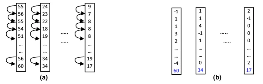
The next step takes the difference between two neighbour values for each column in LL2. This process

is called DBV (Difference Between two Values), which is based on the well-known fact that neigh-bouring coefficients in the LL2are correlated.

Corre-lated values are generally similar, so their differences are small and more data will be repeated, this will be very easy for compression. Eq. (5) represents DBV for each column in LL2. Figure3illustrates the DBV.

DðiÞ ¼DðiÞ Dðiþ1Þ ð5Þ

wherei=1, 2, 3,…_,m-1 andmis the column size of LL2.

2.3 Compress Data by Minimize-Matrix-Size Algorithm

This algorithm is used to reduce the size of the AC-matrix and other high frequency sub-bands. It depends on the Random-Weight-Valuesand three coefficients to calculate and store values in a new array. The following List-1 describes the steps in the Minimize-Matrix-Size-Algorithm:

In the above List-1 the weight values are generated randomly (i.e. random numbers in the range =

{0…_{1}) multiplied with Arr(i) (i.e. represents three} coefficients from a matrix) to produce minimized arrayM(p). The algorithm in List-1 is applied to each sub-band independently; this means each minimized

sub-band is independently compressed. Figure4 illus-trates the Minimize-Matrix-Size Algorithm applied to a matrix.

Before applying the Minimize-Matrix-Size Algo-rithm, our compression algorithm computes the prob-ability of the data for each high frequency matrix. These probabilities are called Limited-Data, which is used later in the decompression stage. The Limited-Data is stored as a header in the compressed file and

are not subject to compression. Figure5illustrates the probability of data in a matrix.

The final step in our compression algorithm is

and one and, when decoded, should reproduce the exact original stream of data. The arithmetic coding needs to compute the probability of all data and assign a range for each, the ranges are limited between Low and High values.

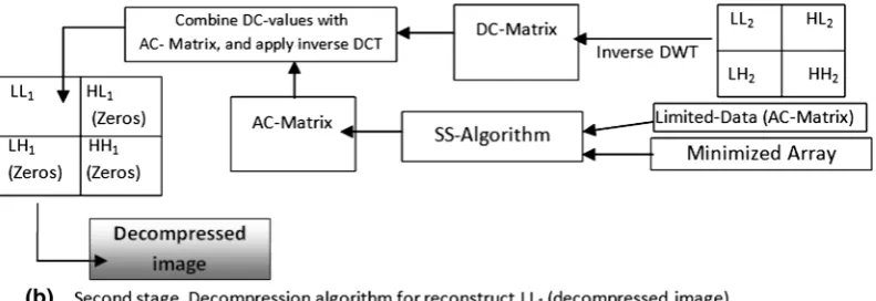
3 The Decompression Algorithm

The decompression algorithm is the inverse of com-pression. The first stage is to decode the minimized array by arithmetic decoding then theLimited Sequen-tial Search Algorithm (LSS-Algorithm) is used to decode each sub-band independently. The LSS-Algo-rithm depends on the Limited-Data array. If the limited data are missed or destroyed, the image could be degraded or damaged. Figure6shows the decom-pression method in a flowchart style.

The LSS-Algorithm is designed to find the original data inside a limited data set, by using three pointers. These pointers refer to positions in the Limited-Data matrix. The initial values of these pointers are 1 (i.e. first location in the Limited-Data matrix). These three pointers are calledS1,S2andS3and are incremented by one in a cogwheel fashion (e.g. similar to a clock, where S1, S2 and S3 represent hour, minutes and

seconds respectively). To illustrate the LSS-Algo-rithm assume that we have the following 293 matrix:

30 1 0

19 1 1

The above matrix will compress by using Minimize-Matrix-Size Algorithm to produce a minimized array M(1)=3.65 and M(2)=2.973, Limited-Data =

{30,19,1,0} and Random-Weight-Values={0.1,

0.65, and 0.423}. Now the LSS-Algorithm will return the original values for the above 293 matrix by using the Limited-Data and the random-weight-values. The first step in the decompression algorithm assigns S1=S2=S3=1, then compute the result of the following equation:

Est¼Wð1Þ LimitedðS1Þ þWð2Þ LimitedðS2Þ þWð3Þ LimitedðS3Þ ð6Þ

whereWis the generated weights andLimitedis the Limited-Data matrix. The LSS-Algorithm computes

Estat each iteration, and compares with M(i). If it is zero, the estimated values are found at loca-tions={S1, S2 and S3} according to Limited-Data. Fig. 4 Ann9mmatrix is minimized into an arrayM

If not, the algorithm will continue to find the original values. This process continues until the end of minimizing array M(I). The algorithm in List-2 illustrates the LSS-Algorithm.

After the high frequency sub-bands are decoded by the LSS-Algorithm, the next step in the decompression algorithm is to apply ABV (Addition between two Values) on the decoded LL2 to return the original

values. ABV represents an inverse equation for DBV (See Eq.5). ABV is applied on each column, which takes the last value at position m, and add it to the previous value, and then the total adds to the next previous value and so on. The following equation defines the ABV decoder.

Dði1Þ ¼Dði1Þ þDðiÞ ð7Þ

wherei=m,(m-1), (m-2), (m-3),…_,2 Then the inverse one-dimensional DCT is applied to each 4 items of data from LL2. Recomposing LL2,

HL2, HL2 and HH2 by inverse DWT yields an

approximation of the original DC-matrix. Next, com-bine each DC value from the DC-matrix with each ([4 94] -1) block from the AC-matrix to generate Table 1 Compressed image sizes using high frequencies in

first level DWT

Image name Original size (MB) Compressed size (KB) Quantization values Low-frequency High-frequency

Wall 3.75 74 0.02 0.02

Wall 3.75 47.6 0.04 0.04

Wall 3.75 33.7 0.08 0.08

Girl 4.14 78 0.02 0.02

Girl 4.14 48 0.04 0.04

Girl 4.14 29.1 0.08 0.08

Woman 4.14 62.1 0.02 0.02

Woman 4.14 38.1 0.04 0.04

Woman 4.14 24.5 0.08 0.08

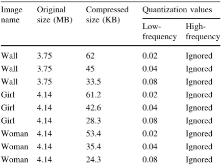
Table 2 Compressed image size without using high-frequen-cies in first level DWT

Image name Original size (MB) Compressed size (KB) Quantization values Low-frequency High-frequency

Wall 3.75 62 0.02 Ignored

Wall 3.75 45 0.04 Ignored

Wall 3.75 33.5 0.08 Ignored

Girl 4.14 61.2 0.02 Ignored

Girl 4.14 42.6 0.04 Ignored

Girl 4.14 28.3 0.08 Ignored

Woman 4.14 53.4 0.02 Ignored

Woman 4.14 35.4 0.04 Ignored

Woman 4.14 24.3 0.08 Ignored

Fig. 7 aA matrix before apply ABV,bapply ABV between two neighbours in each column

(a) 2D BMP “Wall”, dimension 1280x1024 pixels, size=3.75 Mbytes

(b) 2D BMP “Girl”, dimension 1392x1040 pixels, size=4.14 Mbytes

(c) 2D BMP “Woman”, 1392x1040 pixels, size=4.14 Mbytes

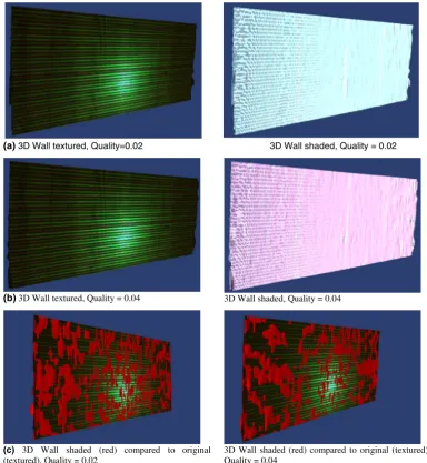
(a) 3D Wall textured, Quality=0.02 3D Wall shaded, Quality = 0.02

(b) 3D Wall textured, Quality = 0.04 3D Wall shaded, Quality = 0.04

(c) 3D Wall shaded (red) compared to original (textured), Quality = 0.02

3D Wall shaded (red) compared to original (textured), Quality = 0.04

(d) 3D Wall shaded (red) compared to original (textured), Quality = 0.08

Fig. 9 aandb3D decompressed image of wall with different quality values.c,dandeDifferences between original 3D wall image and decompressed 3D wall image according to quality

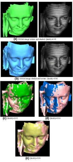
(b)3D Girl image shaded and texture, Quality=0.04

(c)Quality=0.02 (d)Quality=0.04

(e)Quality=0.08

(a) 3D Girl image texture and shaded, Quality=0.02

Fig. 10 aandb3D decompressed girl image with different quality values.c,dand eDifferences between original 3D girl image and decompressed 3D girl image according to quality parameters. Thepinkmodel represents the original background 3D image, whilesother colour

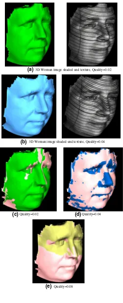
(a) 3D Woman image shaded and texture, Quality=0.02

(b) 3D Woman image shaded and texture, Quality=0.04

(c) Quality=0.02 _(d) Quality=0.04

(e) Quality=0.08

Fig. 11 aandb3D decompressed woman image with different quality values.c,dand

eDifferences between original 3D woman image and decompressed 3D woman image according to quality parameters. Thepink

model is the original 3D woman model whileblue,

green, andgolden models

the matrix LL1, and then apply the inverse

quantiza-tion followed by the inverse two-dimensional DCT on each 494 block from the LL1. The result is the

reconstructed LL1sub-band (Fig.7).

4 Experimental Results in 2D and 3D

The results described below used Matlab for 2D image compression in connection with a purpose-built 3D Table 3 PSNR and MSE

between original and decompressed 2D images

Image name RMSE 3D RMSE Quantization values

Low-frequency High-frequency

Wall 2.49 2.09 0.02 0.02

Wall 2.82 3.95 0.04 0.04

Wall 3.25 4.72 0.08 0.08

Girl 3.09 3.78 0.02 0.02

Girl 4.08 3.94 0.04 0.04

Girl 5.25 3.66 0.08 0.08

Woman 2.88 3.37 0.02 0.02

Woman 3.53 3.09 0.04 0.04

Woman 4.35 2.61 0.08 0.08

Image name MSE 3D RMSE Quantization values

Low-frequency High-frequency

Wall 2.66 2.09 0.02 Ignored

Wall 2.86 3.95 0.04 Ignored

Wall 3.24 4.72 0.08 Ignored

Girl 4.39 3.41 0.02 Ignored

Girl 4.71 3.83 0.04 Ignored

Girl 5.34 3.74 0.08 Ignored

Woman 3.38 3.12 0.02 Ignored

Woman 3.73 3.07 0.04 Ignored

Woman 4.38 2.71 0.08 Ignored

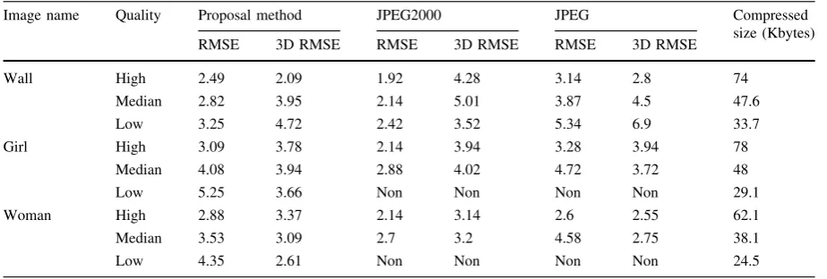
Table 4 Comparison between the proposed algorithm and JPEG2000 and JPEG techniques

Image name Quality Proposal method JPEG2000 JPEG Compressed

size (Kbytes)

RMSE 3D RMSE RMSE 3D RMSE RMSE 3D RMSE

Wall High 2.49 2.09 1.92 4.28 3.14 2.8 74

Median 2.82 3.95 2.14 5.01 3.87 4.5 47.6

Low 3.25 4.72 2.42 3.52 5.34 6.9 33.7

Girl High 3.09 3.78 2.14 3.94 3.28 3.94 78

Median 4.08 3.94 2.88 4.02 4.72 3.72 48

Low 5.25 3.66 Non Non Non Non 29.1

Woman High 2.88 3.37 2.14 3.14 2.6 2.55 62.1

Median 3.53 3.09 2.7 3.2 4.58 2.75 38.1

visualization software running on an AMD quad-core microprocessor. In this research we used three types of images with different dimensions. Our compression algorithm is applied to 2D BMP images. Figure8

shows images tested by our approach, and Table1

shows the compressed size for each image.

The values ‘‘0.02’’, ‘‘0.04’’ and ‘‘0.08’’ refers to high, median and low quality respectively. These values are used by quantization equation (See Eq. 3) to keep high-frequency coefficients (LH1, HL1 and HH1) at first level DWT. If Quality =0.02, this means most of the data remains, otherwise, partial data (a) Decompressed by JPEG2000 3D Flat image (b) Decompressed by JPEG2000 3D Flat image,

Quality=40%, 3D RMSE =4.28 Quality=26%, 3D RMSE=5.01

(c) 3D image decompressed by _{(d) 3D image decompressed by}

JPEG2000 Quality=10% 3D RMSE=3.52 JPEG Quality=56% (degraded 3D)

(e) Decompressed 3D Wall image by JPEG, Quality=26%, 3D RMSE =2.8 [Degraded 3D image]

Fig. 12 a, b and c Decompressed 3D Wall image by JPEG2000, Decompressed image with quality=40 % most of regions are matched with the original image, similarly in quality=26 % and quality=10 % approximately matched

(a) Decompressed 3D image by JPEG2000, Quality=41%, 3D RMSE=3.94

(b) Decompressed 3D image by JPEG2000, Quality=21%, 3D RMSE=4.02

(c)Decompressed 3D image by JPEG, Quality= 45%, 3D RMSE=3.94

(d)Decompressed 3D image by JPEG, Quality=17%, 3D RMSE=3.72 Fig. 13 aand

bDecompressed 3D girl image by JPEG2000.c, dDecompressed 3D girl image by JPEG. For low quality, JPEG cannot reach to compress size

Decompressed 3D image by JPEG2000, Quality=32%, 3D RMSE=3.14

Decompressed 3D image by JPEG2000, Quality=10%, 3D RMSE=3.2

Decompressed 3D image by JPEG, Quality=56%, 3D RMSE=2.55,

Decompressed 3D image by JPEG, Quality=13%, 3D RMSE=2.75 (a)

(b)

(c)

(d) Fig. 14 aand

bDecompressed women image by JPEG2000.c, dDecompressed 3D women image by JPEG. For low quality JPEG cannot reach to compress size

in high frequency sub-bands are discarded, while the low-frequency sub-band depends on the DCT coeffi-cients. Table2shows the effects of high frequencies if ignored from the first level DWT decomposition (i.e. all high coefficients values are set to zero).

The proposed image compression algorithm is applied using a range of quality factors (compression rates) and the recovered images are used for 3D reconstruction and compared to the original 3D models. Figures9, 10 and 11 show the 3D decom-pressed and 3D reconstructed Wall, Girl and Woman respectively. Table3 shows the PSNR and MSE for each 2D decompressed image. Peak Signal to Noise Ratio (PSNR) and Mean Square Error (MSE) are used to refer to image quality mathematically. PSNR based on MSE is a very popular quality measure, and can be calculated very easily between the decompressed image and the original image [10,15].

5 Comparison with JPEG2000 and JPEG Compression Techniques

Our approach is compared with JPEG and JPEG2000; these two techniques are used widely in digital image compression, especially for image transmission and video compression. The JPEG technique is based on the 2D DCT applied on the partitioned image into 8 98 blocks, and then each block encoded by RLE and Huffman encoding [5]. The JPEG2000 is based on the multi-level DWT applied on the partitioned image and then each partition quantized and coded by Arithmetic encoding [1]. Most image compression applications allow the user to specify a quality parameter for the compression. If the image quality is increased the compression ratio is decreased and vice versa [15]. The comparison is based on the 2D image and 3D image quality for test the quality by Root-Mean-Square-Error (RMSE). Table4shows the comparison between the three methods.

In the above Table4‘‘High’’ or ‘‘Median’’ means parameters used by each method is different. Also the ‘‘NON’’ refers JPEG2000 and JPEG method cannot reach to the compress size reached by our approach and still be able to reconstruct the model in 3D. Figures12, 13 and 14 show the 3D decompressed images by JPEG2000 and JPEG.

6 Conclusion

This research has presented and demonstrated a new method for image compression used in 3D applica-tions. The method is based on the transformations (DWT and DCT) and the proposed Minimize-Matrix-Size Algorithm. The results show that our approach introduces better image quality at higher compression ratios than JPEG2000 and JPEG being capable of accurate 3D reconstructing even with very high compression ratios. On the other hand, it is more complex than JPEG2000 and JPEG. The most impor-tant aspects of the method and their role in providing high quality compression with high compression ratios are discussed as follows.

1. Using two transformations, this helped our com-pression algorithm to increase the number of high-frequency coefficients leading to increased com-pression ratios.

2. The Minimized-Matrix-Size Algorithm is used to collect each three coefficients from the high-frequency matrices, to be single floating-point values. This process converts a matrix into an array, leading to increased compression ratios while keeping the quality of the high-frequency coefficients.

3. The properties of the Daubechies DWT (db3) help the approach for obtaining higher compression ratios. This is because the Daubechies DWT family has the ability to zoom-in onto an image, and the high-frequencies sub-bands of the first level decom-position can be discarded (See Table3).

4. The LSS-Algorithm represents the core of our decompression algorithm, which converts a one-dimensional array to a matrix, and depends on the Random-Weight-Values. Also, the LSS-Algo-rithm represents lossless decompression, due to the ability of the Limited-Data to find the exact original data.

5. The Random-Weight-Values and Limited-Data are the keys for coding and decoding an image, without these keys images cannot be reconstructed. 6. Our approach gives better visual image quality

approach removes some blurring caused by multi-level DWT in JPEG2000 [15].

7. The one-dimensional DCT with size n=4, is more efficient thann=8 of JPEG; this helped our decompression approach to obtain better image quality than JPEG.

Also this research has a number of disadvantages illustrated as follows:

1. The overall complexity of our approach leads to increased execution time for compression and decompression; the LSS-Algorithm iterative method is particularly complex.

2. The compressed header data contain floating-point arrays, thereby causing some increase in compressed data size.

Open Access This article is distributed under the terms of the Creative Commons Attribution License which permits any use, distribution, and reproduction in any medium, provided the original author(s) and the source are credited.

References

1. Acharya, T., & Tsai, P. S. (2005).JPEG2000 standard for image compression: Concepts, algorithms and VLSI archi-tectures. New York: Wiley.

2. Ahmed, N., Natarajan, T., & Rao, K. R. (1974). Discrete cosine transforms.IEEE Transactions Computer, 23, 90–93. 3. Al-Haj, A. (2007). Combined DWT-DCT digital image

watermarking.Journal of Computer Science, 3(9), 740–746. 4. Antonini, M., Barlaud, M., Mathieu, P., & Daubechies, I. (1992). Image coding using wavelet transform. IEEE Transactions on Image Processing, 1(2), 205–220. 5. Christopoulos, C., Askelof, J., & Larsson, M. (2000).

Effi-cient methods for encoding regions of interest in the

upcoming JPEG 2000 still image coding standard. IEEE Signal Processing Letters, 7(9), 247–249.

6. Esakkirajan, S., Veerakumar, T., Senthil Murugan, V., & Navaneethan, P. (2008). Image compression using multi-wavelet and multi-stage vector quantization. WASET International Journal of Signal Processing, 4(4), 524–531. 7. Gonzalez, R. C., & Woods, R. E. (2001). Digital image processing. Boston, MA: Addison Wesley publishing company.

8. Grigorios, D., Zervas, N. D., Sklavos, N., & Goutis, C. E. (2008). Design techniques and implementation of low power high-throughput discrete wavelet transform tilters for jpeg 2000 standard.WASET International Journal of Signal Processing, 4(1), 36–43.

9. Rao, K. R., & Yip, P. (1990).Discrete cosine transform: Algorithms, advantages, applications. San Diego: Aca-demic Press. 1990.

10. Richardson, I. E. G. (2002).Video codec design. New York: Wiley.

11. Rodrigues, M., Robinson, A., & Osman, A. (2010). Efficient 3D data compression through parameterization of free-form surface patches. InSignal Process and Multimedia Appli-cations (SIGMAP), Proceedings of the 2010 International Conference on IEEE(pp. 130–135).

12. Rodrigues, M., Osman, A., & Robinson, A. (2013). Partial differential equations for 3D data compression and recon-struction. Journal Advances in Dynamical Systems and Applications, 8(2), 303–315.

13. Sadashivappa, G., & Ananda Babu, K. V. S. (2002). Per-formance analysis of image coding using wavelets.IJCSNS International Journal of Computer Science and Network Security, 8(10), 144–151.

14. Sana, K., Kaı¨s, O., & Noureddine, E. (2009). A novel compression algorithm for electrocardiogram signals based on wavelet transform and SPIHT. WASET International Journal of Signal Processing, 5(4), 11.

15. Sayood, K. (2000).Introduction to data compression(2nd ed.). Morgan Kaufman Publishers: Academic Press. 16. Tsai, M. & Hung, H. (2005). DCT and DWT based image