ABSTRACT
ZUO, XIAOQIU Improving Lumber Cut-Up Manufacturing Efficiency Using Optimization Methods. (Under the direction of Philip H. Mitchell and Myron W. Kelly)
Over the past decades lumber cut-up operations (rough mills), have changed
from using extensive manual decision sawing systems to saws capable of
automated decision making in an effort to save labor cost, increase yield, and
reduce operational mistakes. Although a large amount of automatic and
computerized equipment has been incorporated into rough mills, especially in the
gang-rip first process, many of the process steps still rely on human decision
making. Examples include choosing the appropriate grade of lumber for processing;
designing the optimal arbor for the gang-rip saw; defining suitable part priority values
for the chop saw. This research was conducted based on the hypothesis that these
decisions can be improved through optimization strategies without extra capital
investment.
The first objective of this research was to develop a method to improve the
arbor design on fixed-blade arbor gang ripsaws. The result was the development of
software program - the Gang Ripsaw Optimizer (GRO) written using C++ language.
GRO generates an optimized fixed-blade arbor design for a gang ripsaw that not
only satisfies the cutting bill requirements but also produces a high yield in a
balanced manner. The GRO program reiteratively searches and compares the
optimal part combinations for each lumber width provided by the Romi-Rip simulator,
optimal arbor blade spacing sequence and any part widths that are not included in
the optimal arbor. More than one optimal arbor will be provided in cases where
there are too many widths to be placed on one arbor. The validation results showed
that the GRO program provides overall better solutions than the two other arbor
design software programs, i.e., GRADS and GANGSOLV.
The second objective was to provide a guideline for setting up static priority
values of parts listed in a cutting bill. To develop a system that generates the most
effective priority values (as defined by maximum yield), a study cutting bill with 20
part groups representing the average part sizes and quantities of actual rough mill
cutting bills was created. A 20-factor face-center central composite design with 512
fractional factorial points, 40 axial points and three center points was applied to fit a
second order polynomial model. In addition, a ridge analysis was applied to search
for maximum yield as well as the correspondent critical values. These critical values
were then used to generate the setup formula. Ten cutting bills typically found in
industry were used to validate the new set up system. The results showed that the
static value mode can result in a yield comparable to that given when the dynamic
mode is used. On average, the yield generated from the static value mode was
0.57percent lower than that achieved using the complex dynamic exponential (CDE)
mode, 0.64 percent lower than the simple dynamic exponential (SDE) mode, and
0.39 percent lower than simple dynamic (SD) mode, respectively.
The third objective of this research was to search for the optimal lumber
grade combination that minimizes the raw material and total production cost of rough
problem. Previous research has used linear programming method without verifying
the crucial assumption on simple linearity between yield and grade mix. This study
proved that the simple linear relationship between yield and two-grade and
three-grade lumber combinations does not hold for 90 percent of the industrial cutting bills.
It is, however, impossible to predict the relationship between yield and grade mix
since this relationship is correlated with the characteristics of both the cutting bill and
the combination of lumber grades.
In order to avoid violating the simple linearity assumption, a statistical
optimization method, a five-factor mixture design, was employed to solve the
least-cost lumber grade-mix problem. Five factors (lumber grades) are FAS, SELECTS, 1
Common, 2A Common, and 3A Common. Due to the problems of 3A Common
lumber to obtain enough wider and longer parts, upper bounds as to the amount of
3A Common grade material were applied according to the difficulty levels of cutting
bills. The model creates a lumber grade and cost response surface for all input
solutions. By locating the lowest cost point of the surface, the corresponding lumber
grade or grade mix is obtained. This optimal solution can consist of any number of
different grades and allows the user to pre-specify the lumber grades and grade
IMPROVING LUMBER CUT-UP MANUFACTURING
EFFICIENCY USING OPTIMIZATION METHODS
by
XIAOQIU ZUO
A dissertation submitted to the Graduate Faculty of North Carolina State University
in partial fulfill of the requirements for the Degree of
Doctor of Philosophy
DEPARTMENT OF WOOD AND PAPER SCIENCE
Raleigh
2003
APPROVED BY:
David A. Dickey Urs Buehlmann
Myron W. Kelly Philip H. Mitchell
To my parents
GUOGUANG ZUO and ZHIMIN LU
who care and encourage me and
To my husband
YIHAI LIU
BIOGRAPHY
Xiaoqiu Zuo started her Ph.D. study in the Department of Wood and Paper
Science at the North Carolina State University from Fall 1999. She was working with
Dr. Phil Mitchell and Dr. Urs Buehlmann in the area of Wood Processing. Xiaoqiu
earned her Master's degree in 1997 and Bachelor degree in 1994 from the Chinese
Academy of Forestry and the Northeast Forestry University in China, respectively.
She also obtained a Master’s degree in Statistics from North Carolina State
ACKNOWLEDGEMENT
Sincerest and most heartfelt thanks are extended to my major advisor Dr. Phil
Mitchell, who for four years has inspired, mentored, motivated, and supported me
through various educational, professional, and personal triumphs and defeats.
I have been fortunate to work with Dr. Urs Buehlmann who gave me
guidance, encouragement and support for the past two years.
I am deeply indebted to my co-chair Dr. Myron Kelly for his consistent
supports at various stages of this research.
I owe a special recognition to Dr. David Dickey who is extremely generous in
offering an enormous amount of time and valuable technical advice especially in the
statistical analysis in this research.
I would particularly like to thank Mr. Ed. Thomas for all the technical support
he had provided to me.
I would also like to express my gratitude to Dr. Marcia Gumpertz. Her
kindness and readiness to offer help made this research go smoothly.
My sincere thanks go to my parents Guoguang Zuo and Zhimin Lu, for their
endless care, love and encouragement.
Finally, my deepest thanks also go to my beloved husband, Yihai Liu, for
supporting me, and sharing pain and happiness with me. Thank you for always
Table of Contents
LIST OF TABLES ... IX LIST OF FIGURES ... X
CHAPTER 1. INTRODUCTION ...1
1.1 BACKGROUND...1
1.2 ROUGH MILL OPERATION ...4
1.2.1 ROUGH MILL LAYOUT...5
1.2.2 ROUGH MILL EFFICIENCY...9
1.2.3 MAIN EFFECTS THAT INFLUENCE THE YIELD OF RIP-FIRST PROCESS...13
1.2.3.2.1 Gang-saw operation system...20
1.2.3.2.2 Chop saw operation system ...21
1.2.3.3.1 Cutting bill...23
1.2.3.3.2 Character marks (defect)...24
1.3 OPTIMIZATION AND SIMULATION ...25
CHAPTER 2. HYPOTHESES AND OBJECTIVE ...30
2.1 HYPOTHESES...30
2.2 OBJECTIVES ...31
CHAPTER 3. MATERIALS AND METHODS ...32
3.1 SIMULATION TOOL...32
3.2 LUMBER DATA...32
3.3 CUTTING BILLS...33
3.4 OPTIMIZATION ...34
3.5 STATISTICAL ANALYSIS...35
3.5.1 NUMBER OF REPLICATES...35
3.5.2 NORMALITY INVESTIGATION...36
CHAPTER 4. OPTIMIZING GANG-RIP SAW ARBOR SPACINGS TO IMPROVE ROUGH MILL CONVERSION EFFICIENCY ...38
4.1 BACKGROUND...38
4.2 OBJECTIVE...42
4.5 GRO EVALUATION...52
4.6 LIMITATIONS ...55
4.7 CONCLUSION ...56
CHAPTER 5. STATISTICAL OPTIMIZATION APPROACH TO THE PART VALUE PRIORITIZATION OF OPTIMIZING CHOP SAWS ...58
5.1 BACKGROUND...58
5.2 OBJECTIVE...63
5.3 MATERIALS AND METHODS ...63
5.3.1SIMULATION TOOL...63
5.3.2 LUMBER DATA...64
5.3.3 CUTTING BILL...65
5.3.4 EXPERIMENTAL DESIGN...70
5.3.4.1 Face-centered central composite design ...70
5.3.4.2 Number of replicates ...72
5.4 RESULTS AND DISCUSSION ...73
5.4.1 MODEL INVESTIGATION...73
5.4.2 MODEL ASSUMPTION EVALUATION...74
5.4.3 SEARCH FOR STATIC VALUES...75
5.4.4 GENERATION OF STATIC VALUE SET UP SYSTEM...79
5.5 VALIDATION ...80
5.6 CONCLUSION ...81
CHAPTER 6. APPLYING A MIXTURE DESIGN TO SOLVE THE LEAST-COST LUMBER GRADE-MIX PROBLEM...83
6.1 BACKGROUND...83
6.2 OBJECTIVE...90
6.3 INVESTIGATING SIMPLE LINEARITY ASSUMPTION...90
6.3.1 MATERIALS AND METHODS...90
6.3.1.1 Lumber cut-up simulation...91
6.3.1.2 Cutting bill ...91
6.3.1.3 Lumber data ...93
6.3.1.4 Experimental design...94
6.3.1.4.1 Two-grade combination...95
6.3.1.4.2 Three-grade combinations ...96
6.3.1.5 Statistical analysis...97
6.3.1.6 Verification of findings ...98
6.3.2 RESULTS AND DISCUSSION...99
6.3.2.1 Two-grade combinations...99
6.3.2.1.1 Model assumption investigation ...99
6.3.2.1.2 Results and discussion...99
6.3.2.2.1 Model assumption investigation ...101
6.3.2.2.2 Results and discussion...102
6.3.4 SUMMARY...110
6.4 SOLVING LEAST-COST LUMBER GRAD-MIX PROBLEM ...111
6.4.1 MATERIALS AND METHODS...112
6.4.1.1 Lumber cut-up simulator and cutting bills...112
6.4.1.2 Lumber data ...112
6.4.1.3 Experimental design...112
6.4.1.4 Analysis...113
6.4.1.4.1 Cost calculation ...113
6.4.1.4.2 Model generation...115
6.4.1.5 Performance Evaluation...115
6.4.2 RESULTS AND DISCUSSION...116
6.4.2.1 Buehlmann’s cutting bill ...116
6.4.2.2 Actual industrial cutting bill...118
6.4.3 PERFORMANCE EVALUATION...125
6.4.4 SUMMARY...129
6.5 CONCLUSIONS...130
CHAPTER 7. SUMMARY AND CONCLUSION ...132
7.1 OPTIMIZING THE DESIGN OF GANG RIPSAW FIXED-BLADE ARBORS ...132
7.1.1 SUMMARY...132
7.1.2 CONCLUSION...134
7.1.3 LIMITATIONS AND FUTURE STUDY...134
7.2 OPTIMIZING THE STATIC VALUE SET-UP SYSTEM...135
7.2.1 SUMMARY...135
7.2.2 RESULTS...136
7.2.3 LIMITATIONS AND FUTURE STUDY...137
7.3 SOLVING THE LEAST-COST LUMBER GRADE-MIX PROBLEM...138
7.3.1 SUMMARY...138
7.3.2 CONCLUSION...139
7.3.3 LIMITATIONS AND FUTURE STUDY...140
8 LIST OF REFERENCES...141
9 APPENDICES...154
Appendix 3.1 Ten cutting bills used in this dtudy ...154
Appendix 4.1 Arborgen output for example cutting bill...158
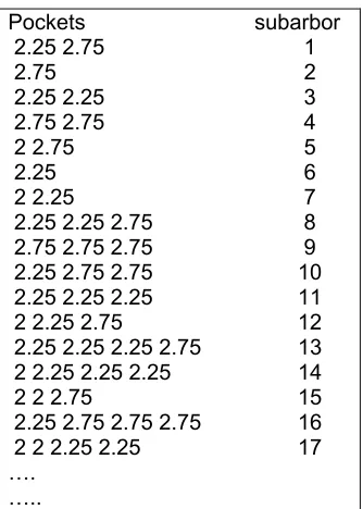
Appendix 4.2 Ranked subarbors generated by GRO...160
Appendix 4.3 Detailed yield comparison between GRO and GRADS...161
Appendix 4.4 Detailed yield comparison between GRO and GANSOLV. ...162
composite design. ...165
Appendix 5.2. Eigenvalues and eigenvectors for the second order polynomial model. ...193
Appendix 6.1. Detailed treatment combinations of mixture designs for two-...194
grade combination...194
Appendix 6.2. Detailed treatment combinations of mixture designs for three- ...195
grade combination...195
Appendix 6.3 Scatter plots for investigating regression model assumption ...196
(two-grade combinations)...196
Appendix 6.4 Scatter plots for investigating regression model assumption ...198
(three-grade combinations). ...198
Appendix 6.5 Design points and experimental results for 5-factor mixture ...200
design with 80 percent upper bound of 3A Common lumber. ...200
Appendix 6.6 Design points and experimental results for 5-factor mixture ...202
design with 60 percent upper bound of 3A Common lumber. ...202
Appendix 6.7 Yields and raw material cost for OPTIGRAMI and the statistical models. ...204
Appendix 6.8 Yields and total production cost results for OPTIGRAMI and the statistical models...205
Appendix 6.9 Costs result for cutting bill F...206
Appendix 6.10 New mixture design for cutting bill F with 40 percent upper...208
List of Tables
Table 1.1. Major component of Hardwood Lumber Grading Rules (NHLA 1998)...15
Table 3.1. Basic Characteristics of ten industrial cutting bills. ...34
Table 4.1. Cutting bill used as an example to demonstrate use of GRO. ...46
Table 4.2. Primary yield Comparison between GRO and GRADS. ...54
Table 4.3. Yield Comparison between GRO and GANGSOLV...55
Table 5.1. Preliminary part groups suggested by Buehlmann (1998). ...67
Table 5.2. The study cutting bill indicating part length and widths (center points) and part quantities. ...69
Table 5.3. The final part groups determined and used by this study. ...71
Table 5.4. The values of three levels for each factor. ...71
Table 5.5. Static values of part group from the initial analysis. ...76
Table 5.6. The new static values for 20 part groups after ridge analysis. ...79
Table 5.7. Value setup formulas for 20 part groups. ...80
Table 5.8. Yield Comparisons between Static Value Mode and Dynamic Modes for ten cutting bills...81
Table 6.1. Number of parts of each size required by the “Buehlmann” cutting bill...92
Table 6.2. Eleven cutting bills used in the study. ...93
Table 6.4. Significance of model parameters when using the "Buehlmann" cutting bill...103
Table 6.5. Cutting bill – three grade lumber combinations with and without linear relationships. ...106
Table 6.6. Basic characteristics of the 11 cutting bills used in this study...107
Table 6.7. The parameters for raw material cost models of the ten cutting bills. ...119
Table 6.8. The parameters for the total production cost models of the ten cutting bills. ...120
Table 6.9. Optimal lumber grade combinations using the statistical model (without... processing cost). ...121
Table 6.10. Optimal lumber grade combinations using the statistical model (with...124
processing cost included)...124
Table 6.11. Optimal lumber grade-mix to minimize raw material cost from OPTIGRAMI. ..125
Table 6.12. Optimal lumber grade-mix to minimize production cost from OPTIGRAMI...126
List of Figures
Figure 1.1. Board width frequency distribution of red oak...2
Figure 1.2. The price of No. 1Common kiln dried hardwoods...3
Figure 1.3. Typical layout of computerized rip-first process...5
Figure 1.4. Typical layout of computerized crosscut first process...6
Figure 1.5. Board cut using the crosscut-first process. ...6
Figure 1.6. Board cut using the rip-first process. ...7
Figure 1.7. Random-length cutting method...12
Figure 1.8. “Force cutting” method...13
Figure 4.1. Relationships among arbor spacings, lumber widths and part widths. ...41
Figure 4.2. Flowchart for GRO program...45
Figure 4.3. Partial Arborgen output. ...47
Figure 4.4. Processed lumber width distribution. ...47
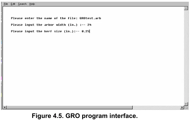
Figure 4.5. GRO program interface...48
Figure 4.6. Partial Arborgen output after ranking. ...49
Figure 4.7. The output of GRO program. ...51
Figure 4.8. Yield table from RR2...52
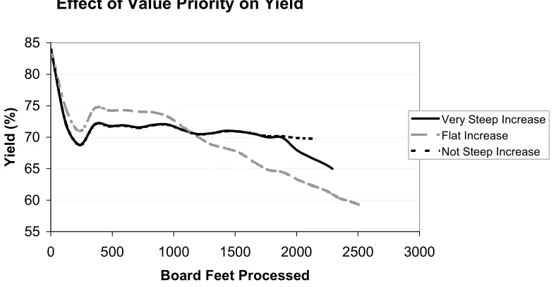
Figure 5.1. Effect of value priority on yield. ...62
Figure 5.2. 1998 kiln dried red oak No.1 Common width distribution...64
Figure 5.3. 1998 kiln dried red oak No.1 Common length distribution. ...65
Figure 5.4. Face-centered central composite design points for three factors. ...70
Figure 5.5. Lack of fit test result from SAS...74
Figure 5.6. Plot of residuals vs. predicted values...75
Figure 5.7. Contour plot for L1W1 and L1W2. ...77
Figure 5.8. 3-D plot for L1W1 and L1W2. ...78
Figure 6.1. Yield prediction nomogram for No.1 Common hard maple...86
Figure 6.2. Mixture design points for testing two grade combinations. ...95
Figure 6.3. Mixture design points for testing three grade combinations...96
Figure 6.4. Mixture design points for testing three grade combinations that includes 3ACommon lumber. ...97
CHAPTER 1. INTRODUCTION
1.1 Background
Wood products have become an important global commodity (Peck 2002). In
the year 2002, the global value of wood products trade was above $200 billion, of
which half of that value was sawn wood, wood-based products and value-added
wood products. In the United States alone, the annual hardwood consumption is
about 11 to 12 billion board feet (Hansen and West 1998). It has been predicted
that by the end of the year 2010, the global wood consumption could increase by 20
percent and more than 50 percent by the end of the year 2020 (Resource
Conservation Alliance). The amount of commercial forest harvesting is increasingly
limited due to growing environmental regulations. Compared to other material such
as steel, concrete, plastic or glass, wood is a renewable raw material that can
continuously supply market demand if managed sustainable. Yet even for the
fastest plantation grown trees at least 15 years is needed to produce a commercially
viable solid wood product (Haygreen and Bowyer 1996). An estimated 95 percent of
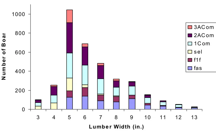
available hardwood lumber is narrower than 10 inches (Figure 1.1) with the average
width less than seven inches (Gatchell 1990b). Meanwhile, the decreasing log sizes
makes lumber producers try to produce more shorter lumber to increase log yield
(Wiedenbeck and Araman 1995). The lumber supplied in the market is narrower,
shorter and lower grade than (Wiedenbeck and Thomas 1995). The shortage of
high quality lumber and increasing demand for lumber drives up lumber cost. Figure
used hardwood species in the United State (Hardwood Market Review 1996 --
2002). As can be seen during this six-year period, the price of No. 1Common red
oak, the mostly used hardwood species, has increased about 10 percent, while the
largest price increase is for cherry at 65 percent. The price for black walnut (not
shown in the graph), has increased by 177 percent from 1971 to 2002 (Schumann
1971; Hardwood Review 2002). In addition, solid wood demand is considered
price-sensitive (Luppold 1983). Wood species utilization has significantly changed in past
decades as a result of the escalating prices. The property of price-sensitivity also
explains the temporary decrease for some species as shown in Figure 1.2.
0 200 400 600 800 1000
3 4 5 6 7 8 9 10 11 12 13
Lumb e r Width (in.)
Nu
m
b
e
r o
f
B
o
a
r 3AC om2AC om
1C om s el f1f fas
No. 1 Common Kiln Dried Hardwoods $400 $600 $800 $1,000 $1,200 $1,400 $1,600 $1,800 $2,000 Au g-96 Fe b-97 Au g-97 Fe b-98 Au g-98 Fe b-99 Aug-9 9 Feb-0 0 Aug -00 Fe b-01 Au g-01 Feb-0 2 Au g-02 $/ M B F Hard Maple Beech Yellow Birch Soft Maple Yellow Poplar Red Oak Cherry
Figure 1.2. The price of No. 1Common kiln dried hardwoods (Hardwood Review 1996-2002).
The United States remains the largest furniture consumer in the world (Smith
and West 1990). Each year, about three billion board feet of hardwood lumber is
used in furniture, cabinetry and millwork (Hansen and West 1998). The hardwood
consumption is expected to increase as the “baby boomers” establish and decorate
their new hones. However, escalating lumber cost coupled with international
competition due to the rapidly expanding global trade in furniture and related
products (Hoff et al. 1997) have caused domestic hardwood dimension
manufacturers much concern and forced them to struggle for their continued
existence.
converted into parts that is subsequently glued, machined, and finished into usable
parts that is distributed to other operations within the factory or to other secondary
manufacturers. The rough mill operation is significantly influenced by raw material
cost and the competitive markets. To be cost competitive, rough mills must produce
parts accurately, efficiently, and in a timely manner.
1.2 Rough Mill Operation
Rough lumber is defined as sawn lumber that has been trimmed and edged
but has not been surfaced. In the context of this work, a rough mill is defined as an
operation generally consisting of multiple rip-cutting and cross-cutting processes that
cut rough lumber into parts of specific size, quality and quantity. These parts are
thereafter typically further machined for use in furniture, cabinets or millwork.
A cutting bill is a customer order that specifies the required part sizes, quality,
and quantities. A cutting is considered a primary cutting if it consists of only
cross-cutting and rip-cross-cutting. A salvage cross-cutting includes additional cross-cutting beyond primary
cutting. Namely, primary parts are cut directly from primary cutting and salvage
parts are cut from remaining unused board areas with additional ripping and
crosscutting steps. The salvage operation is costly but can recover wood which
otherwise would be wasted. Anderson et al. (1992) showed that the average yield
increased 4.3 percent and 5.8 percent for crosscut first and rip-first processes,
respectively, by conducting an extra cutting after the primary cutting. However, this
because the remaining area of a board becomes very small after three-stage
cuttings.
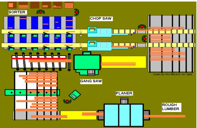
1.2.1 Rough Mill Layout
The conventional layout of a crosscut first rough mill has existed for more
than 50 years. It consists of one or two cut-off saws followed by four or five
straight-line ripsaws (Mitchell 1999a). All equipment is manually operated. Along with the
development of technology, modern rough mills today are equipped with
computerized automatic gang saws and chop saws. The two typical layouts are
rip-first process (Figure 1.3) and crosscut rip-first process (Figure 1.4).
Figure 1.4. Typical layout of computerized crosscut first process. (Courtesy of Mitchell, P.H.)
The cross-cut first process cuts rough lumber first into sections of specific
length at the chop saw, then cuts parts of specific width at the ripsaw from these
sections (Figure 1.5).
Figure 1.5. Board cut using the crosscut-first process. (BC Wood Specialties Group 1996)
Rip Saws Chop Saw Sorter
In contrast, the rip-first operation cuts strips of required width first at the gang rip
saw, and then strips into parts of required length at the chop saw (Figure 1.6).
Figure 1.6. Board cut using the rip-first process. (BC Wood Specialties Group 1996)
Determining which process to apply has been considered one of the most
important decisions in the rough mill (Anonymous 1991). The debate between which
of the two lines is more efficient started during the 1970’s. However, making a
choice between the two layouts is complex, due to the involvement of numerous
effects such as lumber characteristics, part sizes and quantities, the changing nature
of these factors during the lumber cut-up operation, and their interactions. In
general, both processes have advantages. In processing wider and longer boards,
higher yield and productivity are expected in rip-first systems. Rip-first systems do
better jobs for processing species that have more wane, and pith (Wiedenbeck et al
1995; Wiedenbeck 2001). Crosscut-first layouts are good at producing wide parts
from lower grades such as 2A Common and for cutting random width parts to be
glued for panels because it gives better color and grain matching results
efficient cutting species containing spike knots, knot clusters, or larger surface knots
(Wiedenbeck 2001). It is also recommended to crosscut crooked lumber prior to
gang ripping so that part yield can be increased (Gatchell 1990a). Besides these
basic rules of thumb, software such as YIELD (Wodzinski and Hahm 1966), CORY
(Brunner et al. 1989) and RIP-X (Harding 1991) were developed in an effort to
provide guidance on choosing the better process layout for given requirements.
Much research has been conducted related to yield and efficiency of each
process with conflicting results (Huber 1971; Pepke 1980; Hall et al. 1980; Lucas
and Araman 1975). For example, an on-site case study conducted at a clock
manufacturer showed a higher yield using a crosscut - first procedure than a rip-first
procedure (Huber 1971). A similar conclusion was also drawn by Pepke (1980) from
both an actual production line and a computer simulation. A study on cutting fixed
part sizes (Anderson et al. 1992) demonstrated that the yield from the crosscut first
process is consistently higher than that of the rip-first process when only primary
cuttings were considered. However, no yield difference was observed between the
two processes when salvage cuttings were included. Similarly, Lucas and Araman
(1975) claimed that the yield difference between the rip-first and the crosscut first
process was not significant in an interior furniture manufacturing operation. Hall et
al. (1980) also pointed out that either process could produce a better result if various
settings were applied in a stair company.
With the integration of computers, lasers, high speed cameras and
state-of-the-art machinery, higher yield and productivity was reported for the rip-first process
cutting lower grade lumber because the crosscut–first plants have little opportunity to
increase yield with the existing technology (Gatchell 1987). Today’s rip-first rough
mill is a highly technical operation using scanners and computers to control
important steps in the process. The rip-first process has become the dominant layout
in new rough mills during the 1990’s. A survey (Wiedenbeck and Scheerer 1996)
conducted for the wood component industry by the United Sates Department of
Agricultural (USDA), Forest Service, showed that 53 percent of rough mills use the
rip-first process, 36 percent use both rip-first and crosscut first layouts, and 11
percent of them employ the cross-cut first procedure only. The rip-first process was
believed to have a better capacity to handle complex customer orders with a large
number of different part sizes, and large quantity requirement because of its
efficiency in automatic cutting and sorting the final products (Wiedenbeck 2001). In
addition, fewer and simpler decisions from human operators are required in rip-first
processing because it is a more optimized operation. Consequently, the yield and
productivity loss due to error is reduced (Araman and Lucas 1975; Gatchell 1987;
Hall et al. 1980; Hallock and Giese 1980; Mullin 1990). In the current project, only
rip-first processing was studied. Hence the remaining literature review will focus on
rip-first processing of lumber.
1.2.2 Rough Mill Efficiency
Rough mill conversion efficiency is of major importance to the manufacturer.
“The primary objective of a rough mill is to make money, not to cut rough lumber into
would not only favorably impact rough mill profit, but also reduces the demand of
lumber. According to the definition of profit (equation 1.1), increasing the profit is
equivalent to maximizing part value and minimizing lumber and operation cost
(Wengert and Lamb 1994).
Profit = part value - lumber cost - operation cost (1.1)
“Yield is the statistic by which rough mill efficiency is measured” (Hamner et
al. 2002). Though rough mill conversion efficiency is also correlated to lumber cost,
system cost, and acceptable product quality (Huber et al. 1990), experience from
rough mills demonstrates the close relationship between efficiency and yield: higher
efficiency always accompanies a better yield because a higher yield implies less
lumber consumption, and therefore less operational time to produce the same
amount of product. As a measurement of wood utilization, yield directly reflects the
raw material cost, which contributes to more than half of the total cost (Lawser 1993;
Wengert and Lamb 1994; Schumann 1973; Carino and Foronda 1990), and thus
plays an important role in obtaining a higher profit. It was estimated that a one
percent yield increase equals two percent total cost reduction (Kline et al. 1998;
Wengert and Lamb 1994), and a potential reduction in consumption of 30 million
board feet of hardwood lumber in the USA. If interpreted for a mid - sized rough mill,
a one percent yield increase translates into about $150,000 annual savings (Kline et
al. 1998).
Yield is defined as the ratio of the output volume of rough parts and/or panels
to the input volume in board feet of rough dried lumber. Knowing yield of a specific
purchasing lumber and determining manufacturing cost, but is also provides an
understanding of plant capacity and scheduling. The accuracy of the prediction yield
is of principal importance to the rough mill since the lack of current information will
contribute to the improper grade being utilized (Englerth and Dunmire 1966).
Research efforts have been undertaken to predict expected yield of a cutting
bill since the early 1960’s. Thomas (1965) first created yield tables with the
assistance of a computer program (Thomas 1962). Soon after that, a FORTRAN
program was developed to predict the yield for hard maple (Englerth and Dunmire
1966). The most widely used nomogram series for predicting yield of hard maple,
black walnut and red alder were generated by Englerth and Schumann (1969; 1971;
1972). This series of charts allows estimating the yields from lumber that has
thickness other than 4/4 inch and/or the cutting width other than 2 inches. Starting in
the 1980’s, with increasing computing power and programming capabilities, software
programs such as CORY (Brunner et al. 1989), ROMI-CROSS (Thomas 1995c),
ROMI-RIP (1995a; 1995b; 1999a; 1999b), RIP-X (Harding and Steele 1997) were
developed to estimate the yield of lumber cut-up operations. These programs allow
real time simulation of lumber cut up operations and provide yield information,
among others. More accurate yield is obtained from these computer programs than
from the previously developed nomograms (Hoff 2000).
Yields vary when cutting the same part sizes and the same boards for
different part grades. The three most commonly applied part grades are clear
two-face (C2F) cutting, clear one two-face (C1F) cutting, and sound cutting. Clear two-two-face
(C1F) cutting requires defect free cutting on the better side of the part and a sound
cutting on the other side. In a sound cutting, defects such as sound knots, bird
pecks, stain, and pin etc. are acceptable in the parts but no rot, pith, shake and
wane (NHLA 1998). Given the same lumber and part sizes, sound cuttings will
provide the highest yield and clear two face cutting will result in the lowest yield.
Dunmire (1970) reported a two percent yield reduction by substituting C2F cuttings
for C1F cuttings.
When considering cutting patterns, highest yield from a board can be
obtained by cutting and utilizing all of the clear area, as shown in Figure 1.7 (BC
Wood Specialties Group 1996) with waste on only from defects, saw dust, end and
edge trimmings. However, these clear parts may not be useful to customers
because of the unsuitable sizes produced. More often, “force cutting” e.g. cuts of
parts that have specific sizes and quantity requirements are applied in rough mills
(Figure 1.8, BC Wood Specialties Group 1996). Clearly, the yield produced from
“force cutting” is lower than that from random length cutting because of the waste of
clear wood.
Figure 1.8. “Force cutting” method. (BC Wood Specialties Group 1996)
Developing or improving methods to increase “force cutting” yields has
attracted significant interest in both academia and industry. To be successful,
strategies of improving yield require full understanding of the factors that impact
yield. Yield is determined by incoming lumber, process operations, final products,
and their interactions (BC Wood Specialties Group 1996; Buehlmann 1998; Gatchell
1989, 1990a, 1990b; Gatchell et al. 1995, 1996, 1999; Wengert and Lamb 1994;
Wiedenbeck 2001). Methodologies of potential yield improvement shall be
examined from these perspectives. A good understanding of rough mill yield and its
impact factors can help in improving operation guideline and/or technologies.
1.2.3 Main Effects that Influence the Yield of Rip-first Process
Wengert and Lamb (1994) presented ten factors affecting rough mill cost and
yield. These factors from the most important to least important are: lumber grade;
mill layout; kerf; edging practices; lumber size and lumber grading rules. Besides
these effects, lumber species and production scheduling were also considered as
influential factors (Pepke and Kroon 1981). Any changes in these factors can result
in yield gains or losses. In addition, Gatchell (1990a) pointed out the cumulative
effects of lumber lengths, salvage cutting, and saw spacing combination on yield.
The major effects that influence the yield of rip-first process are discussed
below.
1.2.3.1 Incoming raw material
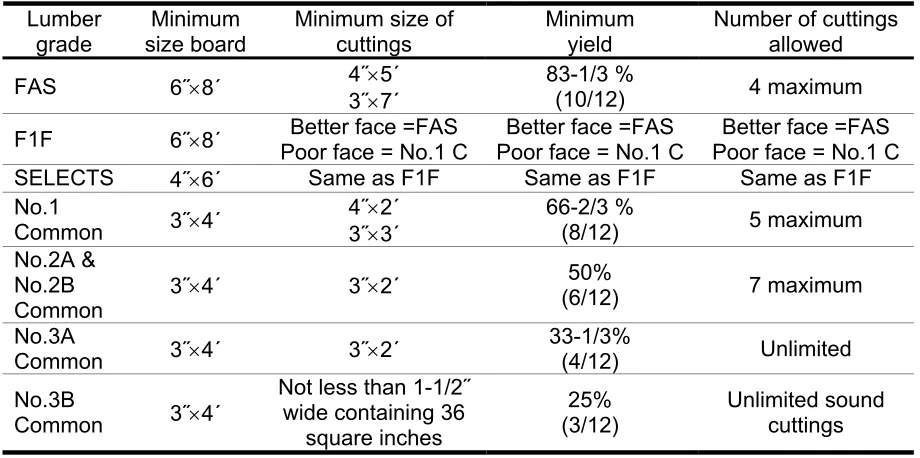
The National Hardwood Lumber Association (NHLA) defines six standard
grades of hardwood lumber based on the minimum size board, minimum size cutting
available, basic yield, number of cuts, and defect constraints (Table 1.1) (NHLA
1998). Among these criteria, the number of defects per board feet is the crucial
indicator of lumber grade (Harding et al. 1993). In order of decreasing quality, the
NHLA grades, in particular, are: FAS; FAS1FACE (F1F); Selects (SEL); No. 1
Common; No. 2 Common (No. 2A Common and No. 2B Common); and No. 3
Common (No. 3A Common and No. 3B Common). F1F and SEL are often used
Table 1.1. Major component of Hardwood Lumber Grading Rules (NHLA 1998).
Lumber grade
Minimum size board
Minimum size of cuttings
Minimum yield
Number of cuttings allowed
FAS 6˝×8´ 4˝×5´
3˝×7´
83-1/3 %
(10/12) 4 maximum
F1F 6˝×8´ Poor face = No.1 C Better face =FAS Poor face = No.1 CBetter face =FAS Poor face = No.1 C Better face =FAS
SELECTS 4˝×6´ Same as F1F Same as F1F Same as F1F
No.1
Common 3˝×4´
4˝×2´ 3˝×3´
66-2/3 %
(8/12) 5 maximum
No.2A & No.2B
Common 3˝×4´ 3˝×2´
50%
(6/12) 7 maximum
No.3A
Common 3˝×4´ 3˝×2´
33-1/3%
(4/12) Unlimited
No.3B
Common 3˝×4´
Not less than 1-1/2˝
wide containing 36 square inches
25% (3/12)
Unlimited sound cuttings
In general, higher grade lumber produces higher yield. Correspondingly,
lower grade lumber generates lower yield, especially for large parts. Lower grades
are thus especially sensitive to changes in required part lengths (Thomas 1965), but
results in satisfactory yields for narrower and shorter parts (Gatchell et al. 1983).
Processing higher grade lumber for a cutting bill that requires longer parts is more
economical and lower grade lumber for a cutting bill with more short parts. The
traditional suggestion is not to process No.2 Common or lower grade lumber for
parts longer than 40 inches. However, Gatchell et al. (1983) revealed that the total
quantity of longer length parts obtained from No.2 Common oak lumber is actually
sufficient to satisfy the dimension part requirements for most furniture cutting bills.
Wood is a heterogeneous material. Each piece of lumber presents a better
end and a poor end (Gatchell et al. 1995; Wiedenbeck et al. 1995). A higher yield is
also been reported that at least 25 percent of kiln-dried red oak lumber has at least
½ inch of crook. Crook lowers yield because crooked lumber is typically aligned at
the rip saw as though it is perfectly straight (Gatchell 1990a; 1990b; Wiedenbeck et
al. 1995). Up to 5 percent of yield can, according to Gatchell et al. (1996) be
recovered if the crook is cross cut before the ripping. In addition to the yield gain,
cutting out the crook part reduces the impact on yield due to the arbor spacing
sequence (Gatchell 1989, 1991).
Grading accuracy is considered the most crucial factor for secondary
manufacturers to make a purchasing decision (Bush et al. 1991). Under NHLA
rules, lumber quality is variable. Among lumber grades, total clear surface area
difference between higher grades such as FAS, SEL, and lower grades such as No.
2A Common and No. 3A Common can be easily visualized. Even within the same
grades, however, lumber quality can be significantly different. An average 7 percent
more yield was gained when comparing “high-quality” to “low-quality” No. 1 Common
and No. 2A Common lumber tested for various cutting bills (Gatchell and Thomas
1997). It was observed that more than 20 percent of the graded No. 1 Common and
No. 2A Common lumber satisfy the maximum grading surface area of the next
higher grade but were down-graded either because of a minor violation on length,
width, or quantity of defects or because of the violation of pith length (Wiedenbeck et
al. 1995; Gatchell and Thomas 1997). The down-graded lumber potentially has
properties similar to the higher grade lumber, and could, therefore, result in higher
In addition to lumber quality, lumber size also plays an important role in
determining process efficiency and cost (Wiedenbeck et al. 1995). Understanding
the relationship between yield and lumber length makes processing more efficient
(Hamner et al. 2002; Wiedenbeck and Araman 1995). The typical lumber length
distribution processed in rough mills is from 8 to 16 feet (Hamner et al. 2002;
Wiedenbeck and Araman 1995), but the feasibility of using lumber shorter than 8
feet has been indicated through simulation modeling (Wiedenbeck and Araman
1995). Englerth and Dunmire (1966) observed that odd length lumber produces
higher yield than even length lumber. Hamner et al.’s results showed strongly that
long boards (15-16 foot) produce higher yield (2002). Therefore, presorting lumber
on the basis of length is one way to benefit yield and efficiency (Schumann 1973;
Wiedenbeck and Araman 1995).
Lumber width was also considered as having an effect on yield
(Pnevvmaticos and Bousquet 1972) since the relative waste from edge strips
increases as lumber width decreases (Wengert and Lamb 1994). However, no
numerical results have been reported so far. Hammer et al. (2002), in their study
contradict the findings by Pnevvmaticos and Bousquest (1972) and Wengert and
lamb (1994) by stating that width does not influence yield.
Lumber species are another factor affecting part yield. The influence of
species is mainly due to defects and defect patterns. The distribution of defects is
not totally random but has certain patterns (Gatchell et al. 1995). For example, pith
lies near the center of the logs and bark is on the outside. Sound knots are close to
more defects, production speed is slower and yield is lower than from a species
having the equivalent grade but having fewer defects (Wiedenbeck and Weidhaas
1996). Investigation on red oak lumber defects (Harding et al. 1993) revealed that
FAS, SELECTS, and F1F have similar sized major defects. No. 3A Common
lumber, however, has significantly larger stain, wane decay, knots, and checks.
More wane was found in lower grades such as No. 1 Common, No. 2A Common and
No. 3A Common than in higher grades. This was explained by the lack of wane
limitation in lower grades (Wiedenbeck et al 1995).
1.2.3.2 Lumber cut up operations
Prior to the introduction of computers in rough mills, all operational decisions
related to the lumber cut-up were made by human operators (Mitchell 2000). Due to
the frequent changing in both lumber and cutting bills, even for a skilled operator,
mistakes or inaccurate operations could occur as a result of fatigue and/or
carelessness. Any mistake in cutting likely creates wood waste. It has become
increasingly difficult for a secondary manufacturer to survive from serious
competition without adopting advanced manufacturing techniques (Hoff et al. 1997).
Much research has been done in an effort to upgrade manual operations with
automatic operations and advanced computerized operations in order to reduce
labor cost, operational mistakes, and improve safety and yields. McMillin et al.
(1984) proposed the Automatic Lumber Processing System (ALPS), that would cut
ALPS was converted into a software program with the same name in 1989
(Klinkhachorn et al. 1989). The program employed several heuristics and proposed
a laser cutting technology to “punch cut” the required parts from any area of the
board, thus result in higher yield. Lin et al. (1994, 1995a, 1995b) also studied the
feasibility and profitability for a processing system that combines hardwood sawmill
and rough mill to process grade 2 and grade 3 red oak logs through cutting yield,
dollar value recovery, production rate, net present value and the internal rate of
return. Results indicated that a direct processing system could be a promising
technique for hardwood value-added manufacturers, especially for those processing
lower grade logs, as long as the combined drying and remanufacturing losses were
less than 19 percent and 28 percent for grade 2 and grade 3 logs, respectively.
Although there is not a completely automatic processing system on the
manufacturing floor yet, many advanced techniques such as applying backgages,
thin kerf saws, processing unedged and untrimmed boards (Kline et al. 1993;
Regalado et al. 1992) have been suggested rough mills to improve the overall yield.
To date, computerized equipment has been introduced into the rough mill for over a
decade. The advantages of employing computerized equipment are, among others:
increased productivity brought by high speed processing; more flexible production;
higher quality products; accurate decision making compared to that of human
operators; the ability to efficiently process complex cutting bills; and the ability to
efficiently utilize lower grade lumber. Kline et al. (1998) reported that a modern
that from simulation software, which is usually believed to be able to produce the
close to or optimum yields.
1.2.3.2.1 Gang-saw operation system
Rising raw lumber cost have stimulated the development and adaptation of
advanced techniques and equipment to increase rough mill conversion efficiency.
The typical technologies adopted to enhance gang-rip saw operations are: lumber
scanning systems; movable fences or moving blade saws; and simulation capability.
The basic idea of scanning lumber is to provide information such as lumber
length, width and shape to assist in locating the best lumber feed position into the
gang saw that will result in the best sawing solution. Among scanning systems, light
or ultrasonic sensors give good measurement on board size, while the location of
major defects in lumber can be detected by video camera(s). Knowing the surface
characteristics of each board, it is possible to determine the best feeding position of
the fence such that the highest volume yield or value is obtained with minimum
waste. Ideally, a machine vision system has the capability to make good decisions
based on complex lumber surface characteristics. However, the heterogeneous
properties of wood, combined with the sensitivity of the machine vision system, can
cause errors in the identification of clear wood as defects which results in yield
reduction (Kline et al. 1998).
The feeding position depends not only on the lumber characteristics but also
on the type of gang saw. There are four types of gang saws: fixed arbor gang saw
saw; and multiple moving blade gang saw. Overall, the fixed arbor system produces
the lowed yield because of the edge loss (Steele and Lee 1994). In recent years,
multiple moving blades gang saws were developed and made available
commercially. The goal of this type of saw is to dynamically position the arbors for
each incoming board so that the defects are grouped into narrow strips (Thomas
1996a). Clearly, a higher yield is expected with the multiple moving blade saws
assuming it is equipped with an accurate scanning system. However, a relatively
longer processing time than fixed arbor system is expected since the blade spacing
needs to be adjusted for each coming board. The fixed arbor with movable fence is
still the most commonly used type pf gang saw in gang-rip first rough mills (Gatchell
1996; Hamner et al. 2002; Mitchell 1998, 1999b; Thomas and Buehlmann 2002).
With this type of saw, the arbor saw spacings are designed and fixed prior to
installing the arbor into the gang saw. Comparing a well-designed arbor that cuts
strips in an optimal manner with minimum edge waste, yield loss due to a poorly
designed arbor could be as high as 7 percent (Mitchell 1998; Gatchell 1996). In
order to change the arbor spacing on a fixed-blade gang saw, the system has to be
shut down, the "old" arbor removed from the saw, and replaced with the newly
designed and set-up arbor. It may take as long as 30 to 40 minutes to replace an
arbor, resulting in downtime that decreases productivity.
1.2.3.2.2 Chop saw operation system
In a rip-first rough mill, the function of the chop saw is to cut strips into parts
size, defects, and grades that are marked manually prior to the chop operation. The
computer then determines the best combination of cutting lengths based on strip
characteristics and cutting requirements that will maximize part volume or part value.
Currently, strip grading is done by marking the symbols for clear, sound, stained,
interior, exterior and rerip onto the strips by human markers at production speed.
The accuracy of marking decisions depends on the markers’ experience, the lumber
grade and cutting bill complexity (Maness and Wong 2002). The marking accuracy
impacts the cut-off patterns and the optimization capacity.
Automatic defect detection has the ability to recognize board characteristics,
locate the defects and construct a digital image of the lumber at a production rate
that allows a highly accurate and efficient chop saw operation. Different
technologies have been employed individually or combined for different functions.
For example, a laser is used to detect the holes, thickness, and profile of the boards;
color video identifies surface defects and discoloration, and X-ray to detect internal
and surface defects by examining the unusual density and internal defects.
In addition to the impact of strip grading accuracy, another important effect on
the computerized chop saw operation is the setting of the part priority values. The
part priority value is used by the saw’s optimization algorithm to make the chop
decisions that determine which parts to cut from each strip or board to maximize
yield or output value. Dramatic yield losses are observed when the only remaining
parts of a cutting bill are long and/or wide because these parts cannot be obtained
from many board sections. Scheduling the cutting order plays an important role in
customer requirements with the available lumber quality and produce the required
part quantities at about the same time. An ideal value setup results in all
requirements being filled simultaneously while obtaining high overall yield.
1.2.3.3 Final products
1.2.3.3.1 Cutting bill
A cutting bill is a customer order which details part width, length, quantity, and
quality studies have shown that cutting bill influences rough mill yield
(Buehlmann1998; Englerth and Schumann 1969; 1972; 1973; Thomas 1965;
Wengert and Lamb 1994). Not only do part sizes and quantity but also the
distribution of part sizes determine part yield (Buehlmann 1998). In general, it was
suggested that the longest parts in a cutting bill influences yield the most (Englerth
and Schumann 1969; 1972; 1973). However, a large requirement of short parts
could lead to higher yield because short lengths fit into existing clear areas between
two defects or the leftover of the larger cutting (e.g. salvage cutting) more easily than
larger parts (Thomas 1965; Wengert and Lamb 1994). Thus, the clear areas of a
board are more efficiently used.
In addition, the geometric characteristics of a cutting bill also determines part
yield. An approach that mixes several cutting bills to expand the choices of the
length and width combinations has been proposed by Wiedenbeck and Scheerer
board are provided when a cutting bill has a variety of width and length
requirements.
1.2.3.3.2 Character marks (defect)
Character marks are natural characteristics of wood. Wood defects such as
sound knots, small holes, small pitch, slight stain or color variation (Kline et al. 1998;
West and Hansen 1996) are allowed when producing hidden interior parts for
upholstered furniture since the main function of these wooden parts is to provide a
frame work of support. The acceptance of character in furniture and other
secondary wood products opens a new area for improving yield and makes it easier
to cut long parts from lower grade lumber. For example, an extra 1.6 percent cutting
area was recovered when certain sound and small unsound defects were allowed in
parts (Kline et al. 1998). In addition, it has been reported that yield change is
positively correlated with the acceptable size and type of the defects and negatively
correlated with the lumber grades (Buehlmann et al. 1998a). For example, average
yield increased 6.5 percent using No.2A Common and 3.2 percent for No.1 Common
if 2 inch defects were accepted. However, in the current solid hardwood furniture
market, character marks are accepted mainly in early American, Western, and
Shaker style furniture even though small character marks frequently appear on one
1.3 Optimization and Simulation
“Optimization is the process of seeking the best solution for a system or
activity” (Biles and Swain 1980). Rough mill optimization is performed to produce
the specified part sizes in required quantities within a limited time at an acceptable
cost (Lamb 1994). A universal optimal cutting pattern can be generated and applied
to all manufactures when the final products are from a homogenous raw material,
such as particleboard (Lamb 1994). Difficulties arise, however, when optimizing the
cut-up of lumber because lumber is a heterogeneous material whose shape and
location of defects vary on each board (Lamb 1994). Meanwhile, irregularities and
lumber characteristics are unpredictable and customer orders change frequently.
A more realistic optimal pattern could be obtained if sample data is directly
observed from the manufacturing floor. However, the feasibility of conducting
studies on an actual production line is constrained by a limited amount of time,
equipment and research budgets. Also, often studies might disturb actual
production, which can only be accepted in rare cases. System simulators allow to
obtain information without disturbing actual operation or is not feasible to observe or
experimentally determined directly (Wiedenbeck 1992a). As a decision support tool
a good simulator should be able to provide accurate evaluation of a new operation;
make a comparison between different systems; predict the performance of
operations with certain constraints; determine the important factors that impact the
operation; optimize the procedures for best outcomes; and observe the bottleneck of
Simulation technique was introduced to the rough mill area in the early 1960’s
(Thomas 1962). By today rough mill simulators have become an important tool to
conduct studies on simulated processing lines to obtain data used to make a
reference for actual rough mills. The use of simulation to model cut-up operations
permits easy and rapid comparative evaluation of either the process, the lumber mix,
or the product (cutting bill) while other factors can be kept constant. Two basic
simulation algorithms in rough mills are flow type and cut-up type (Thomas and
Buehlmann 2002). The flow simulation is aimed to mimic material movement
combined with operator and equipment in a time order. In contrast, a cut-up
simulator is designed to reflect the cut-up of rough lumber producing final parts.
Thomas (1962) developed the first computer program to simulate primary
cutting for a crosscut first rough mill. RIPYLD (Stern and McDonald 1978) was the
first program to simulate the primary cutting for rip-first rough mills. Later programs,
such as CROMAX (Giese and Danielson 1983), Romi-CROSS (Thomas 1998) for
crosscut first process, OPTYLD (Giese and McDonald 1982), MULRIP (Hallock and
Giese 1980), GR-1st (Hoff et al. 1991), AGARIS (Thomas et al. 1994) and ROMI-RIP
(1995a; 1995b; 1999a; 1999b) for rip-first process include, both primary and salvage
cutting operations. Programs YIELD (Wodzinski and Hahm 1966), CORY (Brunner
et al. 1989) and RIP-X (Harding 1991) were designed to allow simulation of both
crosscut first and rip-first process lines.
The early program RIPYLD (Stern and McDonald 1978) can simulate only a
cutting bill limited to 10 part lengths and three specific part widths. Later, the
(Adams et al. 1991) included three types of gang ripping saws named fixed blades,
fixed blades with a movable saw and all blades movable saw. However, it only cut
out random part widths which may not meet customer requirements (Steele and Lee
1994). In AGARIS (Thomas et al. 1994), three different arbor types, 10 part lengths
and three part widths were available. Significant capacity expansion was made with
the ROMI-RIP series (1995a; 1995b; 1999a; 1999b) by providing the ability to
analyze a variety of rough mill processing problems. ROMI-RIP provides six
different types of arbors, six priority methods, 30 part lengths, 10 part widths and
three different part qualities. In addition, it allows changes on ripsaw kerfs and chop
saw kerfs and on the sizes of glued panels.
To efficiently simulate rough mill processing, the key is to identify the clear
areas so that the highest yield of those clear areas can be obtained for the part size
demanded. Although all simulators were developed to simulate manufacturing
processes accurately, various simulation approaches were applied in the simulators.
Englerth and Dunmire’s program locates the defects in a board first and then locates
the clear areas to determine the cutting patterns (1966). Programs YIELD
(Wodzinski and Hahm 1966), YIPLD (Stern and McDonald 1978), CROMAX (Giese
and Danielson 1983), and GR-1st (Hoff et al. 1991) uses a Cartesian coordinate
system to store information of board defects. Anderson described rough mill
processing using a mathematical model that incorporates the production parameters
(Anderson 1983). In program HaRem (Schwehm et al. 1990), a multiple heuristic
algorithm was applied to determine a cutting solution. The ROMI-CROSS (Thomas
length of clear and defect area lines. The run-length encoding method is a data
compression strategy that stores repetitive data, which otherwise would require large
amounts of computer memory. The ROMI-RIP series overcame the limitations of
previous programs and closely simulated rip-first rough mills for both primary
cuttings and salvage cuttings (Thomas 1995a; 1995b; 1999a; 1999b). The
technique employed is called simple lengthwise search for primary cutting and
modified corkscrew method for salvage cutting (Thomas 1995b).
Many programs were designed with special simulation functions beyond the
lumber cut-up process. Programs OFCP (Huber et al. 1977), WALNUT (Martens
1986a), YELLOPOP (Martens 1986b), and OPTIGRAMI series (Martens and Nevel
1985; Timson and Martens 1990; Lawson et al. 1996) are linear programming
computer models that search the optimal lumber grade combinations that minimize
the lumber cost for crosscut first rough mills. MILLSIM1 and MILLSIM2 are able to
estimate the production cost for individual parts according to the explanation
variables defined by users at a crosscut first line (Anderson 1985). HaRem designs
cutting solutions for each incoming board that optimizes the dollar values based on
part sizes, grade, and current market prices (Schwehm et al. 1990).
Among the simulation programs, the ROMI-RIP series (the U.S. Forest
Service Gang Rip First Simulator) developed by Thomas (1995a; 1995b; 1999a;
1999b) is a set of versatile simulation programs that accurately reflect actual rough
mill operations (Thomas and Buehlmann 2002). The program simulates
gang-rip-first operations using digitized boards whose dimensions and defects are expressed
into the gang saw, the program determines the best feed (fence position) to produce
the optimal rip strips and determines the optimal cutting patterns at the chop saw.
ROMI-RIP stops processing when all part requirements are satisfied or all the
boards in the sample batch are processed. The results report the amount of lumber
processed, the cutting operations performed, the number of parts produced and the
CHAPTER 2. HYPOTHESES AND OBJECTIVE
2.1 Hypotheses
It has been predicted that the research priority should be related to
technology and financing information with concentration on automation and yield
improvement (National Hardwood Lumber Association 1996). Although automatic,
computerized equipment has been adopted in rip-first rough mills to improve yield,
efficiency and safety, certain processing steps still mainly rely on human operators’
performance. For instance, before the operation starts, it is the operators’
responsibility to decide which lumber grade or grades should be processed for a
specific cutting bill. This decision significantly affects whether the operation is
economical or not. At the first sawing operation where a board is cut into the
required strips, the arbor spacings of the gang saw are determined and installed by
the operator prior to the beginning of the operation. Next, at the chop saw operation,
the part values must be defined and used by the saw computer to prioritize which
parts are cut. Most of the time these decisions are made without guidelines or other
rules and result in cutting solutions that are not optimal (Wengert and Lamb 1994).
Although modern lumber cut-up operations incorporate computer technology,
2.2 Objectives
The purpose of this study was to use mathematical and heuristic approaches
to improve yield of rough mill processes that typically employ rip-first operations
through improving the accuracy of human decision, rather than use capital
investment of equipment to boost yield. The specific objectives of this study were:
• Develop a software program to aid operators in designing optimal arbor
spacings for the most commonly used gang saws which is fixed arbor with
movable fence;
• Create a static value system to assist operators in defining part priority
values for chop saw operations using a statistical optimization approach; and
• Develop a statistical model to optimize the incoming lumber grade
CHAPTER 3. MATERIALS AND METHODS
3.1 Simulation Tool
Romi-Rip 2.0 (RR2), the U.S. Forest Service Gang Rip First Simulator
(Version 2.0) developed by Thomas (1999) was employed in this study. RR2 was
chosen primarily on the basis of its accurate estimation of yield which provides valid
information that can be used for optimization (Thomas and Buehlmann 2002). The
general settings of RR2 are listed below:
- Salvage cut to primary length and width
- No random-width nor random-length parts
- Continuous update of part counts
- ¼ inch end and side trim on both sides
Other settings were made depending on the project are included in their appropriate
places.
3.2 Lumber Data
Red oak is the most abundant eastern hardwood species (Luppold and
Baumgras 1996) and is, with 39 percent, still the dominant hardwood species used
in the secondary hardwood industry (Vlosky 1996). Even though several thickness
requirements such as 4/4 inch, 5/4 inch, 6/4 inch, 8/4 inch, 5/8 inch, among others,
furniture industry and 70 percent for cabinet companies is 4/4 inch thick (Araman
1982). In this study, therefore, 4/4 kiln dried red oak was employed.
The 1998 Kiln-Dried Red Oak lumber data bank (Gatchell et al. 1998)
contains 3,487 boards in digitized format (20,021 board feet) including FAS, F1F,
SELECTS, No.1 Common, No. 2A Common, and No.3A Common grade lumber. In
order to avoid the impact of crook (side bend) on yield, only boards having less than
¼ inch were included in this data bank. For each project, different lumber sets that
were compared individually were used according to the purpose of each project.
These lumber subsets were constructed by randomly choosing boards from the total
data bank through MAKEFILE, the lumber grouping software tool bundled with RR2
(Thomas 1999a). MAKEFILE allows to customizing lumber files and constructs data
files based on pre-specified percentages of lumber grade, sizes and quantities.
3.3 Cutting Bills
Two study cutting bills that represent the average part sizes and quantities of
industrial cutting bills were used in developing the static value setup system and
solving the least-cost lumber grade-mix problem. The cutting bills are listed in
chapter 5 (statistical optimization approach to the part value prioritization of
optimizing chop saws) and chapter 6 (applying a mixture design to solve the
least-cost lumber grade-mix problem) respectively. To verify or validate the results
generated from this study, ten industrial cutting bills (Thomas 1996a; Wengert and
Table 3.1. Basic Characteristics of ten industrial cutting bills.
Cutting
bill # of parts # of widths
# of narrow widths (? 3.5 in.)
# of wide widths (>3.5 in.)
# of lengths
# of short lengths (? 41 in.)
# of long lengths ( >41in.) 1 5 3 3 0 5 5 0 2 10 4 4 0 9 7 2 3 8 2 2 0 8 5 3 4 5 3 3 0 4 4 0 5 7 3 0 3 3 0 3 6 12 4 3 1 6 4 2 7 16 4 2 2 11 7 4 8 9 5 2 3 4 3 1 9 20 7 5 2 12 7 5 10 25 7 3 4 16 16 0
3.4 Optimization
“Response surface methodology (RSM) is a collection of statistical and
mathematical techniques used for developing, improving and optimizing processing”
(Mayer and Montgomery 2002). It plays a key role in mapping a response surface
over a particular region of interest, optimizing response, or selecting optimal
conditions that satisfy customer requirements. The first application of RSM is to
lower the cost of overall experimentations (Box and Wilson 1951) and is extended
widely to industrial areas where the goal is to find a set of conditions that optimize
(maximize or minimize) the objectives (Giesbrecht and Gumpertz 2001). The first
application of RSM in the forest products industry was 20 years ago when Warren,
Halley and Hancock tried to obtain the optimal lathe parameters to maximize the
veneer yield (Halley et al. 1980; Warren and Halley 1980). This technique was then
used to optimize Oriented Strand Board (OSB), Medium Density Fiberboard (MDF)
and plywood processing by several researchers (Au et al. 1992; Hsu 1996; Park et
producing 3-layer, two species OSB, while Hsu (1996) focused on setting the
optimal pressing parameters such as pressing time, press closing time, and face
moisture content for OSB. Park et al. employed RSM to find the optimal conditions
for higher mechanical properties of MDF (Park et al. 1999). The latest study (Barry
et al. 2001) solved a volatile organic compound (VOC) emission problem during
plywood pressing using Box-Behnken RSM.
In this research, RSM was employed in two separate areas. First, RSM was
used to created static part value set up system that maximizes part yield for
computerized chop saw operation. Secondly, it was used to search for the optimal
lumber grade combination that minimizes raw material cost and total production
cost.
3.5 Statistical Analysis
3.5.1 Number of Replicates
The replication of experiments is regarded as a prime requisite for valid
experimental results (Kuehl 2000). Replication assures the reproducibility of
experimental results; increases the degree of insurance against aberrant
experimental results due to unforeseen accidents; provides the means to estimate
experimental error variance and the capacity to increase the precision for estimates
of treatment means (Kuehl 2000). The number of replications in a research study is
a crucial factor that influences the precision of estimates for treatment means and
Generally speaking, the more replicates the better result. The required number of
replications (r) is determined by the variance (σ2) (which is usually substituted by the
experimental error variance (s2)), the difference between two means (δ), and the
probability of detecting differences δ (β). The formula for calculating the number of
replications for a two-sided test is
2 2( ) ) (
2
2 δ
σ
β
α Z
Z
r ≥ + (3.1)
However, the quantity of replicates is usually constrained by the time and cost
of conducting experiments (Kuehl 2000).
In this research, the detail for the determination of the number of replications
needed is presented in chapters 3 and 4 respectively.
3.5.2 Normality Investigation
For regression models, the important assumptions are that error terms are
normally distributed with mean zero; independent; and have constant variances
(Neter et al. 1996). The validation of analysis from a linear model depends solely on
these assumptions (Kuehl 2000). The violation of any of these assumptions could
lead to erroneous inferences. It is, however, usually uncertain if these features of
the residual are satisfied. Therefore, examining the assumptions of models before
making inferences based on the linear regression model is important. In addition, it
is crucial to check outliers that could skew a fitted line disproportionately toward the
outliers. The examination of a model’s residuals includes tests for randomness,