Model building strategy for logistic regression: purposeful selection

Model building strategy for logistic regression: purposeful selection

Zhongheng Zhang

Department of Critical Care Medicine, Jinhua Municipal Central Hospital, Jinhua Hospital of Zhejiang University, Jinhua 321000, China Correspondence to: Zhongheng Zhang, MMed. 351#, Mingyue Road, Jinhua 321000, China. Email: [email protected].

Author’s introduction: Zhongheng Zhang, MMed. Department of Critical Care Medicine, Jinhua Municipal Central Hospital, Jinhua Hospital of Zhejiang University. Dr. Zhongheng Zhang is a fellow physician of the Jinhua Municipal Central Hospital. He graduated from School of Medicine, Zhejiang University in 2009, receiving Master Degree. He has published more than 35 academic papers (science citation indexed) that have been cited for over 200 times. He has been appointed as reviewer for 10 journals, including Journal of Cardiovascular Medicine, Hemodialysis International, Journal of Translational Medicine, Critical Care, International Journal of Clinical Practice, Journal of Critical Care. His major research interests include hemodynamic monitoring in sepsis and septic shock, delirium, and outcome study for critically ill patients. He is experienced in data management and statistical analysis by using R and STATA, big data exploration, systematic review and meta-analysis.

Zhongheng Zhang, MMed.

Abstract: Logistic regression is one of the most commonly used models to account for confounders in medical literature. The article introduces how to perform purposeful selection model building strategy with R. I stress on the use of likelihood ratio test to see whether deleting a variable will have significant impact on model fit. A deleted variable should also be checked for whether it is an important adjustment of remaining covariates. Interaction should be checked to disentangle complex relationship between covariates and their synergistic effect on response variable. Model should be checked for the goodness-of-fit (GOF). In other words, how the fitted model reflects the real data. Hosmer-Lemeshow GOF test is the most widely used for logistic regression model.

Keywords: Logistic regression; interaction; R; purposeful selection; linearity; Hosmer-Lemeshow

Submitted Dec 30, 2015. Accepted for publication Jan 19, 2016. doi: 10.21037/atm.2016.02.15

Introduction

Logistic regression model is one of the most widely used models to investigate independent effect of a variable on binomial outcomes in medical literature. However, the model building strategy is not explicitly stated in many studies, compromising the reliability and reproducibility of the results. There are varieties of model building strategies reported in the literature, such as purposeful selection of variables, stepwise selection and best subsets (1,2). However, there is no one that has been proven to be superior to others and the model building strategy is “part science, part statistical methods, and part experience and common sense” (3). However, the principal of model building is to select as less variables as possible, but the model (parsimonious model) still reflects the true outcomes of the data. In this article, I will introduce how to perform purposeful selection in R. Variable selection is the first step of model building. Other steps will be introduced in following articles.

Working example

In the example, I create five variables age, gender, lac, hb and wbc for the prediction of mortality outcome. The outcome variable is binomial that takes values of “die” and “alive”. To illustrate the selection process, I deliberately make that variables age, hb and lac are associated with outcome, while gender and wbc are not (4-6).

> set.seed(888)

> age<-abs(round(rnorm(n=1000,mean=67,sd=14))) > lac<-abs(round(rnorm(n=1000,mean=5,sd=3),1)) > gender<-factor(rbinom(n=1000,size=1,prob=0.6),labe ls=c("male","female"))

> wbc<-abs(round(rnorm(n=1000,mean=10,sd=3),1)) > hb<-abs(round(rnorm(n=1000,mean=120,sd=40))) > z<-0.1*age-0.02*hb+lac-10

> pr = 1/(1+exp(-z)) > y = rbinom(1000,1,pr)

> mort<-factor(rbinom(1000,1,pr),labels=c("alive","d ie"))

> data<-data.frame(age,gender,lac,wbc,hb,mort)

Step one: univariable analysis

The first step is to use univariable analysis to explore the unadjusted association between variables and outcome. In

our example, each of the five variables will be included in a logistic regression model, one for each time.

> univariable.age<-glm(mort~age, family = binomial) > summary(univariable.age)

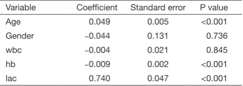
Note that logistic regression model is built by using generalized linear model in R (7). The family argument is a description of the error distribution and link function to be used in the model. For logistic regression model, the family is binomial with the link function of logit. For linear regression model, Gaussian distribution with identity link function is assigned to the family argument. The summary() function is able show you the results of the univariable regression. A P value of smaller than 0.25 and other variables of known clinical relevance can be included for further multivariable analysis. A cutoff value of 0.25 is supported by literature (8,9). The results of univariable regression for each variable are shown in Table 1. As expectedly, the variables age, hb and lac will be included for further analysis. The allowance to include clinically relevant variables even if they are statistically insignificant reflects the “part experience and common sense” nature of the model building strategy.

Step two: multivariable model comparisons

This step fits the multivariable model comprising all variables identified in step one. Variables that do not contribute to the model (e.g., with a P value greater than traditional significance level) should be eliminated and a new smaller mode fits. These two models are then compared by using partial likelihood ratio test to make sure that the parsimonious model fits as well as the original model. In the parsimonious model the coefficients of variables should be compared to coefficients in the original one. If a change of coefficients (∆β) is more than 20%, the deleted variables have provided important adjustment of

Table 1 Univariable analysis for each variable

Variable Coefficient Standard error P value

Age 0.049 0.005 <0.001

Gender −0.044 0.131 0.736

wbc −0.004 0.021 0.845

hb −0.009 0.002 <0.001

the effect of remaining variables. Such variables should be added back to the model. This process of deleting, adding variables and model fitting and refitting continues until all variables excluded are clinically and statistically unimportant, while variables remain in the model are important. In our example, suppose that the variable wbc is also added because it is clinically relevant.

> model1<-glm(mort~lac+hb+wbc+age, family = binomial)

> summary(model1)

The result shows that P value for variable wbc is 0.408, which is statistically insignificant. Therefore, we exclude it.

> model2<-glm(mort~lac+hb+age, family = binomial)

All variables in model2 are statistically significant. Then we will compare the changes in coefficients for each variable remaining in model2.

> delta.coef<-abs((coef(model2)-coef(model1)[-4])/ coef(model1)[-4])

> round(delta.coef,3)

(Intercept) lac hb age 0.029 0.004 0.000 0.004

The function coef() extracts estimated coefficients from fitted model. The fitted model2 is passed to the function. Because there is coefficient for wbc in model1, which has nothing to compare with in model2, we drop it by using “[-4]”. The result shows that all variables change at a negligible level and the variable wbc is not an important adjustment for the effect of other variables. Furthermore, we will compare the fit of model1 and model2 by using partial likelihood ratio test.

> library(lmtest) > lrtest(model1,model2) Likelihood ratio test

Model 1: mort ~ lac + hb + wbc + age Model 2: mort ~ lac + hb + age

# Df LogLik Df Chisq Pr(>Chisq) 1 5 -322.73

2 4 -323.08 -1 0.6867 0.4073

The result shows that the two models are not significantly different in their fits for data. In other words, model2 is as good as model1 in fitting data. We choose model2 for the principal of parsimony. Alternatively, users can employ analysis of variance (ANOVA) to explore the difference between models.

> anova(model1,model2,test="Chisq") Analysis of Deviance Table

Model 1: mort ~ lac + hb + wbc + age Model 2: mort ~ lac + hb + age

Resid. Df Resid. Dev Df Deviance Pr(>Chi) 1 995 645.47

2 996 646.15 -1 -0.6867 0.4073

The results are exactly the same. Because of our simple example, we do not need to cycle the process and we can be confident that the variables hb, age and lac are important for mortality outcome. At the conclusion of this step we obtain a preliminary main effects model.

Step three: linearity assumption

In the step, continuous variables are checked for their linearity in relation to the logit of the outcome. In this article, I want to examine the smoothed scatter plot for the linearity.

> par(mfrow=c(2,2))

> scatter.smooth(age,log(pr/(1-pr)),cex=0.5) > scatter.smooth(lac,log(pr/(1-pr)),cex=0.5) > scatter.smooth(hb,log(pr/(1-pr)),cex=0.5) > scatter.smooth(wbc,log(pr/(1-pr)),cex=0.5)

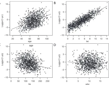
The smoothed scatter plots show that variables age, lac and hb are all linearly associated with mortality outcome in logit scale (Figure 1). The variable wbc is not related to the mortality in logit scale. If the scatterplot shows non-linearity, we shall apply other methods to build the model such as including 2 or 3-power terms, fractional polynomials and spline function (10,11).

Step four: interactions among covariates

that the effect of one variable on response variable is dependent on another variable. Interaction pairs can be started from clinical perspective. In our example, I assume that there is interaction between age and hb. In other words, the effect of hb on mortality outcome is somewhat dependent on age.

> model.interaction<-glm(mort~lac+hb+age+hb:age, data=data,family = binomial)

> summary(model.interaction)

output omitted to save space > lrtest(model2,model.interaction) Likelihood ratio test

Model 1: mort ~ lac + hb + age

Model 2: mort ~ lac + hb + age + hb:age

# Df LogLik Df Chisq Pr(>Chisq) 1 4 -323.08

2 5 -322.91 1 0.3373 0.5614

Note that I use the “:” symbol to create an interaction term. There are several ways to make interaction terms in R (Table 2). The results show that the P value for interaction term is 0.56, which is far away from significance level. When the model with interaction term is compared to the preliminary main effects model, there is no difference. Thus, I choose to drop the interaction term. However, Table 2 Methods to create interaction terms in R

Symbols Remarks

: A simple and direct way to denote an interaction between predictor variables. The formula y ~ a + b + a:b is to predict y from a, b, and the interaction between a and b

* The code y ~ a * b * c can be expanded to y ~ a +b +c + a:b + a:c + b:c + a:b:c. This is a shortcut for all possible interaction terms

^ The code y ~ (a +b + c)^2 can be expanded to y ~ x + z + w + a:b + a:c + b:c. The interaction is in specified degree. In this case, the interaction is defined to be at degree 2

Figure 1 Smoothed scatter plots showing the relationship between variable of interest with mortality outcome in logit scale.

A

C

B

D

lac

wbc age

20 40 60 80 100

100 0

0 2 4 6 8 10 13 14

0 5 10 15

150

50 200 250

10

5

0

−5

−10

10

5

0

−5

−10

10

5

0

−5

−10

10

5

0

−5

−10

hb

Log(pr/(1-pr

)

)

Log(pr/(1-pr)) _{Log(pr/(1-pr))}

if there are interaction effects users may be interested in visualizing how the effect of one variable changes depending on different levels of other covariates. Suppose we want to visualize how the probability of death (y-axis) changes across entire range of hb, stratified by age groups. We will plot at age values of 20, 40, 60 and 80.

> newdata<-data.frame(hb=rep(seq(from=4,to =15),length.out=100,4),lac=mean(lac),age=rep (c(20,40,60,80),100))

> newdata1 <- cbind(newdata, predict(model.interaction, newdata = newdata, type = "link",se = TRUE))

> newdata1 <- within(newdata1, { age<-factor(age)

PredictedProb <- plogis(fit) LL <- plogis(fit - (1.96 * se.fit)) UL <- plogis(fit + (1.96 * se.fit)) })

The first command creates a new data frame that contains new patients. Variables of each patient are artificially assigned. Variable hb is defined between 4 and 15, with a total of 100 patients at each age group. lac is held

at its mean value. The next line applies the fitted model to the new data frame, aiming to calculate the fitted values in logit scale and relevant standard error. The plogis() function transforms fitted values into probability scale, which is much easier to understand for subject-matter audience. Lower and upper limits of the confidence intervals are transformed in similar way. The continuous variable age is transformed into a factor that will be helpful for subsequent plotting.

> library(ggplot2) > ggplot(newdata1,

aes(x = hb, y = PredictedProb)) + geom_ ribbon(aes(ymin = LL,

ymax = UL, fill = age), alpha = 0.2) + geom_ line(aes(colour = age),

size = 1)

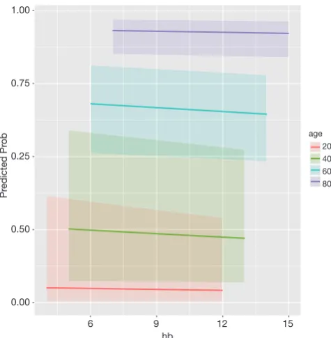
The result is shown in Figure 2. Because there is no significant interaction the lines are parallel. While the probability of death increases with increasing age, increasing hb is associated with decreasing mortality rate.

Step five: Assessing fit of the model

The final step is to check the fit of the model. There are two components in checking for model fit: (I) summary measures of goodness of fit (GOF) and; (II) regression diagnostics. The former uses one summary statistics for assessment of model fit, including Pearson Chi-square statistic, deviance, sum-of-square, and the Hosmer-Lemeshow tests (12). These statistics measure the difference between observed and fitted values. Because Hosmer-Lemeshow test is the most commonly used measure for model fit, I introduce how to perform it in R.

> library(ResourceSelection)

> hoslem.test(model2$y, fitted(model2))

Hosmer and Lemeshow goodness of fit (GOF) test

data: model2$y, fitted(model2)

X-squared = 4.589, df = 8, p-value = 0.8005

The P value is 0.8, indicating that there is no significant difference between observed and predicted values. Model fit Figure 2 Effect of hb on the probability of mortality, stratified by

different age groups.

P

re

di

ct

ed

P

ro

b

1.00

0.75

0.25

0.50

0.00

20 40 60 80 age

6 9

hb

can also be examines by graphics.

> Predprob<-predict(model2,type="response")

> plot(Predprob,jitter(as.numeric(mort),0.5),cex=0.5,yla b="Jittered mortality outcome")

> library(Deducer) > rocplot(model2) > library(lattice)

> histogram(Predprob|mort)

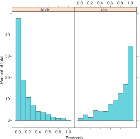
Figure 3 is the plot of jittered outcome (alive=1; die=2) versus estimated probability of death from fitted model. The classification of the model appears good that most survivors have an estimated probability of death less than 0.2. Conversely, most non-survivors have an estimated probability of death greater than 0.8. Figure 4 is the histogram of estimated probability of death, stratified by observed outcome. It also reflects classification of the model. Survivors mostly have low estimated probability of death. Figure 5 is the receiver operating characteristic curve (ROC) reflecting the discrimination power of the model. We consider it an outstanding discrimination when the area under ROC reaches above 0.9.

Summary

The article introduces how to perform model building by using purposeful selection method. The process of variable selection, deleting, model fitting and refitting can be repeated for several cycles, depending on the complexity of variables. Interaction helps to disentangle complex relationship between covariates and their synergistic effect on response variable. Model should be checked for the GOF. In other words, how the fitted model reflects the real

alive die

Predprob

Per

cent of total

0.0

0.0 40

30

20

10

0

0.2

0.2

0.4

0.4

0.6

0.6

0.8

0.8

1.0

1.0

Figure 3 The plot of jittered outcome (alive=1; die=2) versus

estimated probability of death from fitted model.

Jitter

ed mortality outcome

2.0

1.8

1.6

1.4

1.2

1.0

0.0 0.2 0.4 0.6 0.8 1.0

Predprob

Figure 4 Histogram of estimated probability of death, stratified by

observed outcome.

AUC= 0.9325

1-Specificity

0.00 0.25 0.50 0.75 1.00

Sensitivity

Logit (mort ~ lac + hb + age)

1.00

0.75

0.50

0.25

0.00

Figure 5 The receiver operating characteristic curve (ROC)

data. Hosmer-Lemeshow GOF test is the most widely used for logistic regression model. However, it is a summary statistic for checking model fit. Investigators may be interested in whether the model fits across entire range of covariate pattern, which is the task of regression diagnostics. This will be introduced in next article.

Acknowledgements

None.

Footnote

Conflicts of Interest: The author has no conflicts of interest to declare.

References

1. Bursac Z, Gauss CH, Williams DK, et al. Purposeful selection of variables in logistic regression. Source Code Biol Med 2008;3:17.

2. Greenland S. Modeling and variable selection in

epidemiologic analysis. Am J Public Health 1989;79:340-9. 3. Model-building strategies and methods for logistic

regression. In: Hosmer DW Jr, Lemeshow S, Sturdivant RX. Applied logistic regression. Hoboken, NJ, USA: John Wiley & Sons, Inc., 2000;63.

4. Zhang Z, Chen K, Ni H, et al. Predictive value of lactate

in unselected critically ill patients: an analysis using fractional polynomials. J Thorac Dis 2014;6:995-1003. 5. Zhang Z, Ni H. Normalized lactate load is associated

with development of acute kidney injury in patients who underwent cardiopulmonary bypass surgery. PLoS One 2015;10:e0120466.

6. Zhang Z, Xu X. Lactate clearance is a useful biomarker for the prediction of all-cause mortality in critically ill patients: a systematic review and meta-analysis*. Crit Care Med 2014;42:2118-25.

7. Kabacoff R. R in action. Cherry Hill: Manning Publications Co; 2011.

8. Bendal RB, Afifi AA. Comparison of stopping rules in forward regression. Journal of the American Statistical Association 1977;72:46-53.

9. Mickey RM, Greenland S. The impact of confounder selection criteria on effect estimation. Am J Epidemiol 1989;129:125-37.

10. Royston P, Ambler G, Sauerbrei W. The use of fractional polynomials to model continuous risk variables in epidemiology. Int J Epidemiol 1999;28:964-74. 11. Royston P, Altman DG. Regression using fractional

polynomials of continuous covariates: parsimonious parametric modelling. Applied Statistics 1994;43:429-67. 12. Hosmer DW, Hjort NL. Goodness-of-fit processes

for logistic regression: simulation results. Stat Med 2002;21:2723-38.

Cite this article as: Zhang Z. Model building strategy for