University of Twente
EEMCS / Electrical Engineering
Control Engineering
Design of a Capacitive based Closed-Loop
Displacement Sensor
Johan Schabbink
MSc report
Supervisors:
Design of a Capacitive based Closed-Loop
Displacement Sensor
- iii -
CONTENTS
Contents
iii
Chapter 1:
Introduction
11.1Capacitive based displacement sensing in MEMS 1
1.2Closed loop sensing concepts 2
1.2.1 Concept 1: Translational version 2
1.2.2 Concept 2: Rotational version 4
1.2.3 Concept 3: Pull-in version 6
1.3Goal of this research 7
1.4Thesis outline 8
Chapter 2:
Modelling of system elements
9
2.1 Introduction 9
2.2 System overview 10
2.3 Transducer model 12
2.4 Rotational suspension and structure model 16
2.5 Moment actuator 18
2.6 Angle sensor 19
2.7 Concluded design directions 24
Chapter 3:
MEMS based structure design
25
3.1 Introduction 25
3.2 Design and structural parameters 26
3.2.1 Transducer design 26
3.2.2 Suspension design 29
3.2.3 Sensor design 30
3.3 Mechanical system design 32
3.4 Conclusions and results 35
Chapter 4:
Dynamic system behaviour
36
4.1 Introduction 36
4.2 System block diagram 37
4.3 Angular displacement control-loop 37
4.3.1 Open-loop transfer 38
4.3.2 Closed-loop behaviour 41
4.4 Displacement sensor behaviour 43
- iv -
4.6 Conclusion
46
Chapter 5:
Conclusions and outlook
47
5.1 Thesis objective 47
5.2 Conclusions 47
5.3 Outlook and recommendations 49
References 50
Appendix A:
Capacity and forces between non parallel plates
51
Appendix B:
Derivation of a second order spring-damper suspension
54
Appendix C:
Suspension tuning
57
Appendix D:
Sensor optimalization
59
- 1 -
CHAPTER 1
INTRODUCTION
1.1 Capacitive based displacement sensing in MEMS
MEMS is the acronym for Micro Electro Mechanical Systems. The term MEMS-devices refers to parts or systems like: sensor, actuator, micro-fluidic systems and mechanical mechanisms. The typical feature size is around micrometers, while the overall device dimension is in the range of millimetre. These devices are typically manufactured using lithography based processing, alike the semiconductor processes. Due to the large area to volume ratio, electrostatic forces rule over inertia and mass, giving electrostatic forces in MEMS a practical application.
Capacitive based sensing is a method to measure a displacement by means of an electromagnetic field enclosed between two or more electric guiding plates. For common capacitive based sensing the capacitance change due to a displacement, which can be measured.
The application of electrostatic forces is generally used for actuation, less common the electrostatic force is used for displacement sensing. This type of displacement sensing however is used in this research.
If due to displacement one of the electric guiding plates that encloses the electric field is shifted, a force change occurs between the plates.
A visualization of this situation is given in Figure 1-1. With a setup where both plates are parallel to each other and located parallel to each other, there is a force Fx that pulls the plates
over each other to a maximum overlap and a force Fy that pulls the plates against each other.
One or both of these forces can be used to measure displacement.
- 2 -
There are various ways to improve the resolution of a capacitive sensor. The obvious way is to add more plates and therefore multiplying the resolution by the number of plates added. Another way is to increase the area of the plates or to decrease the gap between the plates. The capacity of any number of plates N with area A and gap g is given by the equation:
0
2 rA
C N
g ε ε
= (1.1)
With ε0 the vacuum permittivity and εr the relative permittivity of the matter between the
plates.
With multiple plates, a comb-like structure arises as shown in Figure 1-2.
Figure 1-2 Multiple plates in a comb-like setup, the comb-drive.
In a setup like in Figure 1-2 the total capacity of the structure depends on two times the number of (dark gray) plates because each plate has two neighbouring plates. These structures are typically used structures in the field of MEMS.
1.2 Closed loop sensing concepts
Prior to this research, three concepts where developed. These three concepts are discussed in this section. The concepts where the introduction to the in this report presented results. The most promising concept was chosen to be designed.
1.2.1 Concept 1: Translational version
- 3 -
Figure 1-3 Translational concept
Features:
• To keep the shuttle at a fixed position by means of a voltage feedback Ua, which is used as the measure of external displacement Δx.
• The internal position state z is measured by the linear comb capacitor.
• Reference voltage Ut is fixed.
Assumptions:
• The translational shuttle moves without tilting.
• The internal sensor holds the sensitivity achieved during tests
Electrostatic forces: between the opposite teeth and ε0 the vacuum permittivity.
Transducer plates:
The condition for static equilibrium (regardless of the suspension stiffness)
comb p
- 4 -
Which is solved for U Ua: a =β
(
l z Ux,)
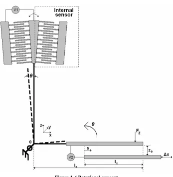
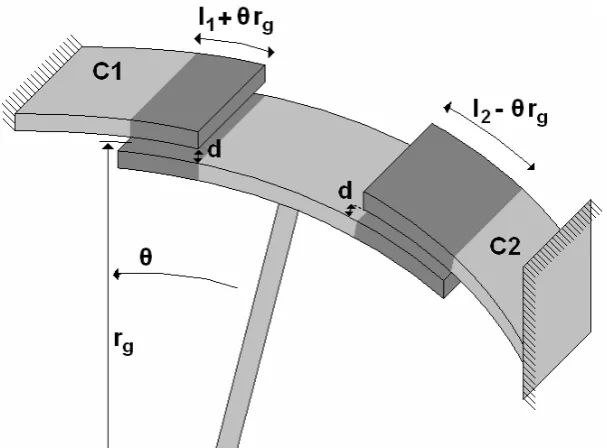
⋅ t (1.5)1.2.2 Concept 2: Rotational version
Figure 1-4 Rotational concept
Features:
• To keep a constant angle θ by means of a voltage feedback Ua, which is used as the measure of external displacement Δx.
• The rotation angle θ is measured by the internal capacitive position sensor (rotational comb fingers).
• The reference driving voltage Ut is fixed.
Assumptions:
• The rod and plate rotate without deforming.
- 5 -
The front transducer
Starting from the parallel position the initial capacitance 0 0
(
)
0
The capacitance varies due to the rotation angle θ.
( )
cos(
0)
When applying voltage Ut, the electrostatic moment about the centre of rotation ‘0’ is
( )
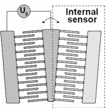
2The rotational comb-drive actuator
Figure 1-5 The rotational comb-drive actuator/sensor
The capacitance between a single pair of fingers
( )
0(
0)
The total capacitance amounts to
( )
0(
0)
0(
0)
=
∑
, the effective rotational radius.- 6 - sensitivity given by
( )
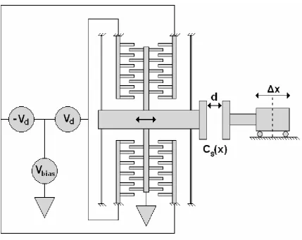
0The third concept is analogous to the tunnelling-based position sensing method known for STM (Scanning Tunnelling Microscope) shown in Figure 1-6.
Figure 1-6 Pull-in concept
Features:
• To keep the capacitance Cs(x) constant by moving the left plate and follow the
movement of the right plate
• The driving voltage Vd on the comb drives is used as a measure of external
displacement Δx.
- 7 - Assumptions:
• The capacitance measuring signal exerts no influence on the balance.
• The capacitance can be measured with the resolution achieved during tests
Finding Vd as a function of x and Cs
Unlike the previous two concepts, the displacement x is directly coupled into the sensing capacitance:
Electrostatic force by comb drives in the linearized configuration:
( )
0When the capacitor plate on the right side is offset by x, in order to keep the constant sensing capacity C xs
( )
, the left plate also has to be displaced by:supposing a suspension stiffness km.
Thus, the driving signal Vd(x) can be solved as a function of x.
According to W. Zhou [1] the coupling of the displacement into the internal state with concept 1 and 3 three does not introduce as much nonlinearity as in concept 2, the rotational version. Based on this conclusion this research was started with the design phase of the rotational concept.
1.3 Goal of this research
The goal of this research is:
• To design a capacitive based closed-loop sensing system based on the rotational
concept discussed in section 1.2.2
- 8 -
• The input signal bandwidth is 10 Hz.
• The sensing system should not be larger than the dimensions of 1mm x 1mm=1mm2 so
that the sensor can be implemented into complex MEMS devices.
In order to fulfill these requirements, dimensions of elements and parts have to be scaled down to the minimum obtainable.
1.4 Thesis outline
This thesis is setup with three main chapters, the chapters 2,3 and 4. Appendix D elaborates on the subject of optimization and miniaturization of comb sensors in the line of this research.
In chapter 2 the concept this thesis started on is divided into system elements. For each element a physical model is created which in the following chapters is used to design the structure. The laws of electromagnetism and transducer science are combined with design principles to model the individual elements.
In chapter 3 from the individual system elements a MEMS-structure design is made. The allowed area is separated to place each element. A structure is designed, and the separate elements are designed into the carrier structure. The chapter results in a MEMS-structure with all the system elements integrated.
In chapter 4 the dynamic system behavior is analyzed. The controller is designed in this chapter to make the MEMS-structure stable during operation. The system is first analyzed in an open-loop situation, next the loop is closed, and the controller is adjusted to obtain the required bandwidth. In the last step the system-loop is analyzed (differs from the open/closed-loop). Again the controller is adjusted to improve performance.
- 9 -
CHAPTER 2
MODELING OF SYSTEM ELEMENTS
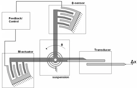
The outline of this chapter is to create the tools in formula form to design and develop the device . The, in the previous chapter, discussed concept that represents the start of this thesis will be modelled. The concept is divided into four parts: The transducer section consisting of the translating and rotating plate, the suspension and rigid body, the angle sensor and the moment-actuator of which the steering signal will also be used for the displacement measuring.
2.1 Introduction
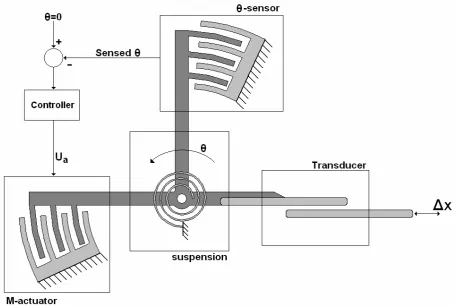
In Figure 2-1 the concept for the MEMS-structure is given, with the separate parts placed in boxes. There are four separate main functions, which are:
• The transducer that couples the movement x to a negative moment over θ that rotates the suspended structure.
• The angle θ-sensor that performs capacitive angle measurement in order to find the moment introduced by the transducer
• The moment M-actuator that generates a positive moment to correct the negative
moment the transducer introduced, because of this action the plates should remain parallel.
• The suspension that allows 1 degree of freedom in the θ direction and cancels the other degrees of freedom.
- 10 -
Figure 2-1 Concept overview of the MEMS-system with its four main function parts
2.2 System overview
To fill in the empty place between the angular sensor and the M-actuator, a controller is integrated. This controller “closes the loop”, it checks the sensor for a rotation over θ and send a correction signal to the M-actuator to return the angle θ back to zero.
The specifications of this controller will be determined later on in chapter 4.
In order to keep the plates as parallel as possible, an as sensitive as possible angular rotation sensor, the θ-sensor, is needed. The goal for this part will be to maximize the capacity change
dC with respect to the displacement dx: max Csensor
x ∂
⎡ ⎤
⎢ ∂ ⎥
⎣ ⎦
- 11 -
Figure 2-2 Concept of the system with the MEMS-system and the controller
The concept works in the following way:
Through an external displacement the lower plate moves with Δx inwards. Due to the
displacement the overlap of the two plates changes. The moment balance around the rotation point disappears and an angle θ, depending on the overlap-change, exists.
Then this angle θ is measured with the θ-sensor. This “error” angle is the input of the controller that tries to keep the error as low as possible. In fact the controller tries to get the upper plate back to the initial parallel position. It can do so by sending a steering signal to the M-actuator that changes the moment and returns the balance.
- 12 -
2.3 Transducer model
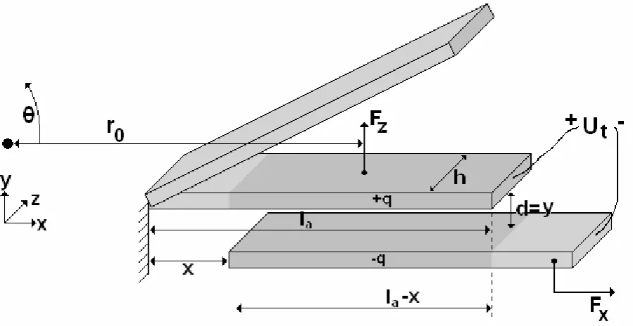
The first part of Figure 2-1 is the transducer built with two parallel plates. It works accordingly:
If the lower plate moves in direction x, outward, a change in force between the plates appears, the upper plate rotates with angle θ around its fixed rotating point and the parallel situation disappears.
A 3D zoom of the plates is given in Figure 2-3 to illustrate the variables.
To find the forces that are acting on the shuttle section that transfers movement x and force F to the lower plate, a transducer will be used.
The ports interesting for this transducer are the relation between x and θ keeping the voltage U constant. Then q follows the capacity like q CU= . The quantities force F and torque T are variables that are not interesting at this point and will be treated later in the actuator design.
Figure 2-3 Exaggerated situation during operation of the transducer section
For θ =0 when the plates are parallel, the parallel plate capacity arises:
(
)
0(
)
From origin the transducer is a three-port transducer, but because the controller keeps the plates parallel, the work of the third port is zero, because when θ =0 then A Td= θ =0, and cancels out. That this assumption holds is proven in Appendix A.
- 13 -
During operation θ =0 (controlled situation) only 2 ports remain active, this gives the energy function:
The co-energy function for this transducer is described by Elwenspoek & Krijnen [17] as:
' 1 2
2
transducer t
E = − CU J (2.3)
From equation 2.3 the acting forces Fx, Fy and Fz can be calculated by taking the partial derivative with respect to the corresponding dimension with the gap d in the y direction
The force in each direction is:
t
The force Fy at radius r0 generates a moment Mt around the point of rotation according.
0
Due to the pull-in effect also a stiffness is present in the transducer.
(
)
(
)
- 14 -
To evaluate if the parallel plate equation 2.1 holds for a relative small parallel plate, a series of simulations has been done. The simulations are performed with a finite element method simulation tool to analyze the EM-fields [7]. The dimensions used during the simulation runs are:
With the given dimensions 15
0 2.5 10 F
C = × − and 15
,0 3.5 10 F
sim
C = × − .
The influence of a small angle between the plates is given in Figure 2.4.
Figure 2-4 The normalized capacitance as a function at the angle θ
- 15 -
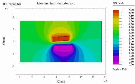
Figure 2-5 The field distribution of a non-parallel plate capacity
Also a difference between the simulated value and the analytical model is found to be
3D 1.4
G = , which represents a correction factor for small finite plates with given parameters.
The for finite parallel plates with similar dimensions adjusted infinite plate equation becomes:
(
)
0(
)
To increase the change of moment per displacement unit Mt
x ∂
∂ , multiple plates can be used in a fork-like setup. With a number of Nt gaps the moment becomes:
(
)
Assuming all radii ri are equal, the change of moment per displacement unit with radius rt then becomes:
- 16 - For indication with a displacement of the 1nm goal:
(
)
In chapter 3 these variables will be optimized
2.4 Rotational suspension model and structure model
The second part of Figure 2-1 is the suspension. It consists of a rotational spring that holds the structure free to rotate from the underlying bulk. The ideal suspension is very stiff in all degrees of freedom except the rotation θ. In this rotation direction the suspension should be very compliant. A zoom on the rotational part from Figure 2-1 is given in Figure 2-6.
Figure 2-6 A zoom on the suspension
- 17 -
Figure 2-7 A sketch of the suspension with the parameters relevant for the rotational stiffness k
The rotational stiffness θ for the setup in Figure 2-7 is:
(
)
(
)
3 2 2
1 3 3
8
12 1
Ehw a a
k
l
θ
ν − + = ⋅
− Nm (2.18)
With an out of plane stiffness of:
3 3
2E h w c
l ⋅ ⋅
- 18 -
2.5 Moment actuator
The third part of Figure 2-1 is the M-actuator or moment-actuator. The actuator is constructed out of two circular bended plates that rotate over each other. The principle works alike the translational comb-drive. The setup and variables are given in Figure 2-8
Figure 2-8 The M-actuator in a schematical representation
The energy of the M-actuator from Figure 2-8 is described in equation 2.20:
(
)
The M-actuator generates a moment depending on the voltage Ua and the angleθ ≈0
according:
If all radii ra are equal, then:
- 19 - Where N is the number of gaps.
The actuator moment Ma total, depends on the input voltage Ua according:
, 0
The moment balance between the M-actuator and the transducer, which is a function of the steering voltage Ua of the m-actuator then becomes:
, ,
a total t total
M =M [-] (2.25)
The static dependence of actuator voltage Ua with respect to the displacement x for approximation of the displacement is:
(
)
- 20 -
the moment actuator. The difference with the moment actuator is that the change in capacitance is now measured. The setup and variables are given in Figure 2-9.
Figure 2-9 The rotational sensor
The capacitance of the sensor shown in Figure 2-9 is:
( )
0h l(
o)
C
d
ε θ
θ = + F (2.32)
The total energy equals:
(
)
This setup generates a moment around the point of rotation of:
0 2
The moment generated by the sensor is constant and does not depend on angle θ. This
moment causes a disturbance to the balanced structure, and therefore to the measured angle. This is not desirable, therefore an adjustment was made.
The sensor will be build in a differential setup which also eliminates the drift of the sensor by exterior influences,.
- 21 -
Figure 2-10 The differential rotational sensor
The total energy of this setup consisting of two separate sensors is:
( )
2( )
2 1 2 1 1 2 21 1
2 2
s C C
E =E +E = C θ U + C θ U J (2.35)
Usually U1=U2 then the energy becomes:
( )
( )
2 1 21 2
s s
E = ⎡⎣C θ +C θ ⎤⎦U J (2.36)
The behaviour of the capacitance for a differential setup is given in Figure 2-11. This setup only measures the difference between two identical sensors, removing all common effects.
- 22 -
Then Es becomes:
(
)
Which is independent of the angle θ, so the sensor moment Ms is:
0
To increase the sensitivity of the sensor, multiple teeth can be used.
In Figure 2-12 a sketch is given of a differential angle sensor with multiple teeth (and gaps).
- 23 -
With N the number of gaps between the teeth. When l1=l2, a symmetrical sensor setup, then:
The sensitivity of the sensor can now be found according:
( )
( )
From equation 2.44, it can be concluded that to maximize the sensitivity the number N should be high because a number of N gaps results in N times more accuracy.
Also the radius ri has to be large. The h and the d need to be respectively the maximum obtainable structure height and the smallest possible gap. The resulting current needed to measure the capacity change can be calculated from the charge q of the total energy:
2
1 1
2 2
E= CU =qU ⇒ =q CU J (2.45)
The current that flows as a result of the charge change becomes:
0
- 24 -
2.7 Concluded design directions
All the parts of Figure 2-1 are now discussed and analyzed. The conclusions for each part are summarized in this section.
The moment Mt of the transducer part with respect to the displacement x needs to be maximized, this is done by increasing the number of teeth, and the initial overlap.
The rotational stiffness θ is built of a perpendicular placed set of leaf-springs which has a low rotational stiffness.
The M-actuator is used to balance the total moment of the structure, which is the sum of the negative moment the transducer generates and the positive moment the actuator generates.
To eliminate the drift and the moment caused by a normal plate sensor, the sensor will be build with a differential setup. To get the maximized sensitivity the radius and the number of teeth-pairs for sensing are maximized.
These conclusion will be used as directions for designing the MEMS-structure.
- 25 -
CHAPTER 3
MEMS BASED STRUCTURE DESIGN
In this chapter the structure design will be discussed. The design direction and equations created in the previous chapter will be used to define the structure parts. The outline of this chapter describes the path from a set of specifications and equations to a theoretical working structure under ideal circumstances.
3.1 Introduction
The schematical overview of the system is given in Figure 3-1. The MEMS system consisting of the front-transducer, the θ-sensor, the M-actuator and the structure with suspension all displayed in Figure 3-1 will be designed.
- 26 -
A perpendicular leaf spring suspension setup is used because of the low stiffness, see Figure 3-2.
With a spring setup like this, three empty area’s are left, in these area’s the transducer, the sensor and the actuator should be placed. The sensor is the most important part for obtaining a high resolution and requires the more space for a higher resolution, therefore it will be placed in region 2, the largest region.
The transducer and actuator must be placed opposite of each other, but can be interchanged. To stay with the setup used in Figure 3-1, the transducer will be placed in region 1 and the actuator in region 3 shown in Figure 3-2, but interchanging them makes no difference.
Figure 3-2 The suspension setup
3.2 Design and structural parameters
3.2.1
Transducer design
To increase the moment Mt the transducer generates due to electrostatic attraction, multiple plates instead of one are used.
This increases the moment to N times the original moment.
,
t tot t
M = ⋅N M Nm/- (3.1)
Another way to increase the moment Mt is to increase the radius r0.
0
t t
M = ⋅r F Nm/- (3.2)
- 27 -
a factor two. The load on the shuttle in the direction of Δx cannot be eliminated, since this load generates the moment, and therefore the rotation of the structure.
Figure 3-3 The shuttle section balanced by a second transducer
The symmetrical setup as shown in Figure 3-3 is used to keep the shuttle, represented by the middle plate, in balance. The plate is in balance if:
1 2
the structure is in balance and the forces in y-direction cancel each other out.
- 28 -
Figure 3-4 The transducer with the shuttle section in dark gray
One leaf spring used in the folded flexure has a stiffness in the displayed Δx direction of:
3 3
With The Young’s modulus of silicon: 11 2
1.30 10
E = × N m . And where l is the length of a
single leaf-spring, w the thickness and h the height. The stiffness in the y direction is:
N/m
With A the cross section area.
The stiffness in the z direction (up down direction in the Figure 3-5) is:
3 3
Which represents the out of plane stiffness.
- 29 -
Figure 3-5 The folded flexure setup for straight guidance, for eliminating the other 5 degrees of freedom
The folded flexure has to be stiff enough to reduce the movement error due to the electrostatic forces that pull the parallel plates inward, to far below 1 nm. According:
,
3.2.2
Suspension design
The suspension of the structure is realized with two perpendicular placed leaf-springs. The maximum allowed area of the structure is 1 mm2. With the symmetrical setup only half the area can be used, shown in Figure 3-6
Figure 3-6 The suspension setup with perpendicular leaf-springs and stiffness reduction
- 30 - This leaves a maximum length for the leaf-springs of
2 2 6 6
max 0.5 0.5 20 10 687 10 m
l = × − × − = × − (3.10)
for the leaf-spring. The rotational suspension stiffness then becomes:
(
)
The a factor then becomes 1.03. The rotational stiffness for this setup then results in:
(
)
And the out of plane stiffness for the rotational part then becomes:
3 3
With E the Young’s modulus, h the height, w the width and l the length of the leaf-springs.
3.2.3
Sensor design
With the maximum allowed space represented in Figure 3-6 the maximum size or radius of the angular sensor is also defined, shown in Figure 3-7.
- 31 -
Since the capacity change ΔC depends on the radius, as much as possible sensor-combs should be placed at the largest radius. Placing sensing-combs at the inner half-circle is of almost no use, therefore this room shall be used for beams that support and stiffen the sensor-combs and the rest of the structure.
With the sensor-teeth dimensions given in Figure 3-8a the amount of differential pairs can be calculated.
The space each capacitor takes is 29 micrometer in length/radius and 10 micrometer in width.
a) b)
Figure 3-8 a)The dimensions of the sensor teeth in micrometers b) ten fingers placed in a row
If ten teeth are placed in a row, as shown in Figure 3-8b a sensor bank can be created. Each bank of teeth has 20 differential gaps and 21 separate teeth. The height of each sensor bank is
21 teeth 5 μm 3 μm gap 108 μm× + = .
If for instance the bank is placed in the largest ring, the effective radius ri is 446 micrometer, creating a the sensitivity SC (equation 2.44) of
( )
( )
- 32 -
Figure 3-9 Illustration of the rotational sensor part
For example, in the illustration in Figure 3-9 are twenty sensor banks placed. This will result in a total sensor sensitivity of 20⋅SC =42.12 pF.
3.3 Mechanical system design
The centre of gravity, needed to calculate the inertia of the rotating part of the sensor is shown in Figure 3-10. The centre of gravity can be generated by Solidworks.
- 33 -
The structure is more or less half a cylinder, Fokker [12] determines the inertia of a cylinder in the centre of gravity as half the mass times radius squared.
The structure is only half a cylinder therefore it has approximately half the inertia in the centre of gravity.
2
1 1 2 2
COG
J = ⋅ m r⋅ kgm2 (3.16)
The inertia of the rotating part of the MEMS-structure is:
(
)
2 2 2 2 , , ,
Q COG COG COG x COG y COG z COG
J =J + ⋅m r =J + ⋅m r +r +r kgm2 (3.17)
With this inertia, and the stiffness of the suspension, the resonance frequency than become:
tot
- 34 -
- 35 -
3.4 Conclusions and Results
To ensure a minimal load on the shuttle section that transfers the displacement to measure, the structure needs to be in balance. The forces in y-direction than cancel each other out, and the shuttle is minimally loaded in this direction.
The load on the shuttle in the direction of Δx cannot be eliminated, since this load generates the moment, and therefore the rotation of the structure.
Straight guidance of the shuttle section is required because the load sideways is eliminated by means of a symmetrical setup, but the shuttle section can still tilt or shift in other dimension then the desired Δx without straight guidance.
Since the capacity change ΔC depends on the radius, as much as possible sensor-combs should be placed at the largest possible radius.
- 36 -
CHAPTER 4
DYNAMIC SYSTEM BEHAVIOUR
In this chapter the dynamic behaviour of the structure will be discussed, starting with the open-loop system. Next the loop is closed than the system loop is analyzed to complete the design. The chapter ends with the appearing disturbances and the reaction of the complete system to these disturbances.
4.1 Introduction
The last part of the sensor that needs to be defined is the controller. A sketch of the complete system, with all the external connection included, is given in Figure 4-1. The output-signal of the controller is the steering signal for the M-actuator, which is also used as a measure for the displacement.
For the controller a PID-regulator with a low-pass filter is used. The controller brings stability to the until this point unstable system, and keeps the transducer plates parallel. Hereafter the disturbances are defined, and modelled, to predict their behaviour.
- 37 -
4.2 System block diagram
The complete sensor system is given in Figure 4-2. The system input Δx [m] and output Ua [V] are outside the control-loop. The input for the open-loop is the desired angle θsetpoint and the output is the measured angle θ*.
Figure 4-2 Block diagram of sensor system. The control-loop is used to keep MEMS structure at a zero rotation with help of a moment actuator
The dynamics of the structure are incorporated into the block MEMS dynamics. Also the influence of the, by the transducer introduced, negative stiffness is implemented into this block.
In the following sections the system in Figure 4-2 will be discussed with respect to it’s dynamical behaviour. The standard control engineering approach will be used, starting with the open-loop system, then closing the loop and finally adding the external influences and disturbances.
4.3 Angular displacement control-loop
The control-loop of the system is shown in Figure 4-3. The control-loop is built out of 4 blocks. When transformed to the control engineering scheme Ha HMEMS and Hs are together the plant and HPI+ is the controller.
- 38 -
4.3.1
Open-loop transfer
The specified system bandwidth is set at 10Hz, the MEMS-system resonance frequency is not fixed during the design phase, and is set to 1000 Hz. The reasoning will be discussed later on. Therefore an obvious initial bandwidth setting for the controller is 100 Hz.
Initial PI settings:
V s
1000 0.000159
rad rad
p i
K = τ =
For the controller shown below in equation 4.1
1
This controller has the dynamical characteristics shown in the Bode plot in Figure 4-4.
Linear System Bode Plot
100 1000 10000
Figure 4-4 The Bodeplot of the dynamic behaviour of the PI controller
The actuator part Ha has the transfer function: (equation 2.24):
, 0
- 39 -
The MEMS-system (see also Appendix B) behaves according:
2
The system is still under design and parameters can still be adjusted. To ensure stability and optimal control-behavior, the resonance frequency should be set very high, in the order of 100 kHz. Because the resonance frequency corresponds to the flexure suspension, this high resonance frequency decreases the resolution of the system. A safe trade-off is to set the resonance frequency, and thereby the suspension stiffness, on f=1000 Hz. With the inertia generated by Solidworks, I =1.5 10× −13 kgm/-, the total suspension stiffness k
θ needs to be:
5.921 10 0.2169 10 5.921 10
suspension t
- 40 -
Linear System Bode Plot
100 1000 10000
Figure 4-5 The Bodeplot of the dynamic behaviour of the MEMS system
The transfer function of the sensor part can only be approximated. The complete systempart that measures the angle consists of the physical sensor part in the MEMS structure combined
with the instrumentation that transforms the capacity change to the rotation angle θ*.
Therefore Hs approximately acts to rotation as
*
The transfer function of the open-loop system in Figure 4-3 is:
( )
*( )
( )
With the separate blocks the transfer function becomes:
ol PID a MEMS s
H =H ∗H ∗H ∗H - (4.14)
With Ha and Hs constants
- 41 -
Linear System Bode Plot
100 1000 10000
Figure 4-6 The open-loop Bodeplot Hol
The open-loop system is stable, with a resonance frequency of the MEMS system at 1000Hz. The phase at the zero dB crossing is approximately -90 degrees. The controller bandwidth is 121 Hz.
4.3.2
Closed loop behaviour
To determine the controller settings, the open-loop system discussed in the previous section has to be closed. A block diagram of the closed-loop system is given in Figure 4-3. Compared to the open-loop system, several components are of importance now, because they are part of the system in the closed-loop situation.
The transfer function of the control-loop is determined by:
( )
- 42 -
Linear System Bode Plot
10 100 1000 10000
Frequency (Hz)
10 100 1000 10000
Frequency (Hz)
Figure 4-7 The closed-loop Bodeplot Hcl
To reduce the resonance peak a second order low-pass filter will be added, creating a PI+ controller. The characteristics of the filter are according to Soemers, van Dijk and de Vries [14] determined by the equations:
1000
- 43 -
Linear System Bode Plot
10 100 1000 10000 100000
Frequency (Hz)
10 100 1000 10000 100000
Frequency (Hz)
Figure 4-8 The closed-loop Bodeplot Hcl with PI+ controller
It is possible to increase the bandwidth of the closed control-loop, but when the bandwidth is increased, the phase margin decreases and the system oscillation thereby increases. If the bandwidth is even further increased, the phase lag will be -180 degrees and the system behaves as an oscillator.
4.4 Displacement sensor behavior
- 44 -
Figure 4-9 The block-diagram of the closed loop displacement system with in- and output.
The M* block is the block that translates the voltage Ua to the displacement Δx (equation 2.31):
Input transducer block Ht
, 0 2
The transfer function of the sensor-system with output Ua is determined by:
1
- 45 -
Linear System Bode Plot
10 100 1000 10000 100000
Frequency (Hz)
10 100 1000 10000 100000
Frequency (Hz)
Figure 4-10 The sensor system closed-loop Bodeplot Δ Δ
cl
x * S =
x
Depending on the final system requirements, the controller has to be tuned.
4.5 Disturbances
Two types of disturbances act on the sensor-system.
The first type is a uncertainty in the accuracy of the sensor, because the θ-sensor has a certain minimum measurable capacitance. This uncertainty gives a disturbance.
The sensor has an accuracy of
0
From test results derived during a similar research it proved that the minimum detectable capacitance change per bank is 1.0675 10 F× −16 at 1 Hz.
This sensor inaccuracy results in a Gaussian disturbance to the sensor signal.
The noise level is:
- 46 - with respect to the signal.
The second noise source originates from the temperature. If a structure is suspended very compliant, the internal motion of the molecules sets the structure in motion, this motion is called the Brownian motion. The generated noise is dependent on the total stiffness of the structure with respect to the fixed world.
In the MEMS-structure there are multiple compliances, the compliance of the suspension and the stiffness in the transducer that is balanced by a stiffness introduced by the controller.
The Brownian motion is with:
0
And the total rotational suspension stiffness of 5.921 10 6
suspension
k = × − Nm/rad
Which is a stiffness suspension suspension2 37.006
suspension
With the results produced in this chapter the capacitive based closed-loop sensor is complete. There is one remark to this system, because the system input Δx is outside the control-loop. Therefore the system input acts as a disturbance on the control-loop, making it impossible to power up both the controller and the system at the same time. However this can be easily solved by a RC-timing circuit in the instrumentation.
Since the system input Δx acts as a disturbance, the control loop input is the desired angle θ0. The output is the measured angle θ* acting as error signal for the controller. The steering signal of the controller to correct the error signal is used as a measure for the input displacement Δx .
The open-loop control system is stable, with a damped MEMS resonance frequency.
The desired system bandwidth of the input signal is 10 Hz according to spec. To be on the safe side, the controller bandwidth has to be at least 100 Hz. The closed loop control system has, after tuning the controller, a bandwidth of 183 Hz see Figure 4.10, which is even better than the previously wanted control-loop bandwidth.
- 47 -
CHAPTER 5
CONCLUSIONS AND OUTLOOK
The overall conclusions on this thesis will be presented in this chapter, together with the recommendations for further improvements on the design. Specific conclusions on the different subjects have been given in the individual chapters.
5.1 Thesis objective
The goal of this research is to develop a capacitive based closed-loop displacement sensing device, in order to improve the resolution of a common capacitive sensor.
The in advance created approach still holds:
• Analytical studies of the different concepts
• Choice on basis of the theoretical analysis
• Proposal for practical embodiment(s)
• Analysis of practical embodiment
• Optimization of the design
5.2 Conclusions
As part of the Multi Axes Micro Stage project, the design and fabrication of a 6 DOF manipulator in MEMS technology capable of nanometre resolution positioning was developed. In order to obtain a resolution in the nanometre range, an accurate displacement sensor with preferably sub-nanometre precision is required. Since common capacitive based MEMS sensors can not obtain such a resolution, at a micrometer displacement range, without very large sensor dimensions, a new principle was developed.
feed-- 48 feed--
back of the position of the balance, which is used to control the voltage of the actuator. By designing the balance such that its rotational compliance is high, small shuttle position changes lead to relatively large open-loop rotations of the balance, which can be measured by the capacitive sensor.
The sensor consists of five parts: the flexure suspension, the transducer, the angle sensor, the actuator and the controller.
The suspension allows the sensor to rotate. A compromise had to be made for this part. A displacement at the input generates a force change between the transducer-plates. This force change causes the suspended structure to rotate, therefore it has to be as compliant as possible to maximize the open-loop angular rotation. But a very compliant suspension results in a very low resonance frequency of the suspended structure. A very low resonance frequency of the structure between 20 and 30 Hz makes it almost impossible to avoid oscillation, because the input signal varies between 1 and 10 Hz. This is essentially a trade-off between the compliance of the suspension and the resonance frequency of the structure.
Another way to maximize the open-loop angular rotation is by applying a higher transducer voltage between the front transducer plates. The force between the plates depends on the voltage-squared, but the rotational negative stiffness existing between those plates also depends on this voltage-squared, possibly leading to instable behaviour.
Note that if the transducer voltage is increased, the number of teeth in the actuator should also be increased to counteract the increased force between the transducer-plates.
Now the angle of rotation per displacement unit is determined, it is measured as accurate as possible. This task is performed by the angle sensor part.
To minimize temperature, humidity effects and other external influences the sensor is composed of two capacitive sensors that are used as a differential sensor. With this principle the angle is represented by the difference of the currents that flows in and out of the capacitors, at a fixed voltage, caused by the charge change.
The rotational negative stiffness cannot be compared to a mechanical negative stiffness. First of all, the stiffness depends on the applied voltage-squared. Second, the stiffness depends linear on the overlap of the two transducer-plates. Third, the stiffness depends on the effective
transducer radius-squared according:
(
)
2(
)
,t t, , t t t,
kθ U x r = ⋅r c U xθ .
This research has produced the design of a compact sensor system with a resolution of 1 nanometre at bandwidth of at least 10 Hz. The area the system requires for reaching these
specifications is 1mm×1mm=1mm2.
The designed system configuration used during simulations has a stroke of 20 micrometre in both directions which allows a total stroke of 40 micrometres. With a small design adjustment this total stroke could be increased to 100 micrometres.
- 49 -
obtained. The etching is based on Deep Reactive Ion Etching (DRIE) to create vertical anisotropic etch profiles with an aspect ratio up to 1:20.
A high resolution displacement sensor system which requires only little space, can easily be integrated into larger MEMS systems where accurate displacement sensing is needed.
5.3 Outlook and recommendations
The next step for the completion of this sensor system is the design of a prototype. The various possibilities all described in the previous chapters have to be carefully weighted and an optimal system design has to be found. Especially the leaf-spring suspension is a very critical parameter. The suspension both influences the resolution of the system as well as the resonance frequency.
The front transducer can be expanded with some extra parallel plates, to improve the resolution. If the sensor system is made at the largest possible size 1mm x 1mm the transducer could have as much as 20 teeth per sensor-part.
The actuator has to be adapted to the transducer forces. If the transducer voltage or the number of teeth is increased, the actuator needs more teeth to counteract the increased input forces.
For a prototype also various end-stops have to be implemented, to prevent the structure from pull-in instability and avoid irreparable damage to the prototype.
If a prototype has been produced, the controller needs to be adjusted to the system characteristics.
To connect the sensor, a set of instrumentation in the form of electronics has to be developed. A very important issue for the electronics is that the controller needs to be active and running, when the voltage over the transducer is increased from zero to the desired voltage.
The complete system can be activated at once only if the end-stops are properly in place. The controller will then be able to returning the rotating part back to the parallel position by applying an actuator force.
- 50 -
5.4 References
[1] W. Zhou, A Study of Several Capacitive-Based Closed-loop Position Sensing Concepts [2] R.P. Feynman, R.B. Leighton, M. Sands, The Feynman lectures on physics volume II [3] M.N.O. Sadiku, Elements of Electromagnetics
[4] B.R. de Jong, A Six Degrees of Freedom MEMS Manipulator
[5] D.M. Brouwer, Design Principles for six Degrees-of-Freedom MEMS-based Precision Manipulators
[6] A.A. Kuijpers, Micromachined Capacitive Long-Range Displacement Sensor for Nano-Positioning of Microactuator Systems
[7] http://www.flexpde.com
[8] K.E. Petersen, Silicon as a Mechanical Material, Proc. IEEE vol. 70 no. 5 [9] M.P. Koster, Constructiepricipes voor het nauwkeurig bewegen en positioneren [10 http://www.ioffe.rssi.ru/SVA/NSM/Semicond/Si/mechanic.html
[11] R.L. Huston, Multibody Dynamics
[12] A.D. Fokker, Time and Space, Weight and Inertia: A chronogeometrical introduction to Einstein’s theory
[13] I.F. Lutters-Weustink, CAD/CAM Handleiding Solidworks deel I
[14] H.M.J.R. Soemers, J. van Dijk, T.J.A. de Vries, Mechatronic Design of Motion Systems [15] Stephen M. Barnes, Samuel L. Miller, M. Steven Rodgers, Fernando Bitsie, Torsional
Ratcheting Actuating System, Sandia National Laboratories
[16] R. Kassies, Atomic Force Fluorescence Microscopy Combining the best of two worlds [17] M. Elwenspoek, G. Krijnen, Introduction to mechanincs and transducer science
[18] W.B.J. Zimmerman, Process Modeling and Simulation with Finite Element Methods [19] C.W. Steele, Numerical Computation of Electric and Magnetic Fields
- 51 -
APPENDIX A
CAPACITY AND FORCES BETWEEN NON
PARALLEL PLATES
In chapter 2 the assumption was made that the front transducer plates are kept parallel. If the plates are not aligned parallel, the model needs to be changed to a 3 port transducer. In order to validate the simplification of the model, an analysis was made. Again is started with the transducer shown in Figure A1.
Figure A-1 Exaggerated situation during operation of the front transducer section
The parallel plate capacitance depends on the effective area of the plates, spanned by the overlap la-x and the width h, the permittivity ε0 and the initial gap d. For a setup like this, the angle of rotation θ also is important, because it effects the effective gap d and the effective overlap length la-x.
- 52 -
In this equation two different situations can be distinguished, namely θ =0 and θ ≠0 . First θ =0 when the plates are parallel used in chapter 2, the parallel plate capacity arises:
( )
cos(
0)
(
)
0The second situation when θ ≠0 an angle between the plates exists and the angle θ plays a role in both the overlap length lx and the gap z0:
( )
(
)
(
)
When this 3 port transducer is described in it’s co-energy form as used in chapter 2.
The co-energy function for this transducer is described by Elwenspoek & Krijnen [17] as:
(
)
From equation A.4 the acting forces Fx, Fy and Fz can be calculated by taking the partial derivative with respect to the corresponding dimension with the gap d in the y direction The force in x direction is:
t
The force in y direction is:
- 53 -
The force in z direction is:
t
The force Fy at radius r0 generates a moment Mt around the point of rotation according.
0
Due to the pull-in effect also a stiffness is present in the transducer.
,
This stiffness is translated to a rotational stiffness:
- 54 -
APPENDIX B
DERIVATION OF A SECOND ORDER
SPRING-DAMPER SUSPENSION
The basic principle of the dynamics of the MEMS-structure given in Figure 4-3 is given in Figure B-1.
Figure B-1 The basic principle of the MEMS-system
The differential equation for this structure is:
Homogeneous differential equation
2
Inhomogeneous differential equation
2
Two parameters are introduced :
2
0
k b
I I
ω = γ = (B.3)
The first parameter, ω0, is called the (undamped) natural frequency of the system . The second parameter, γ is called the damping ratio.
- 55 -
The external force can be expressed as:
( )
0cos( ) i t
t t
S ωt =S t =S eω (B.7)
The equation now becomes:
2
If the angle θ is also written in a constant term and a time dependant term,
( )
t( )
0 ei tωFrom this equation follows that:
0
The amplitude of the resulting angular rotation θ0 can be written as:
- 56 -
The behavior of the system depends on the relative values of the two fundamental parameters, the natural frequency ω0 and the damping ratio Γ. The dependence on both parameters is given in Figure B-2.
Figure B -2 The system response for Γ settings
The four curves shown in Figure B -2 are known as:
Critical damping
When Γ = 1, ω is real, the system is said to be critically damped. A critically damped system converges to zero.
Over-damping
When Γ > 1, ω is still real, but now the system is said to be over-damped. An over-damped system will take longer to return to zero than a critically damped door would.
Under-damping
When 0 ≤ Γ < 1, ω is complex, and the system is under-damped. In this situation, the system will oscillate at the natural damped frequency ω0, which is a function of the natural frequency and the damping ratio. The system will return to zero.
Instability
- 57 -
APPENDIX C
SUSPENSION TUNING
This addition will is used to tune the rotational suspension stiffness. If necessary the resonance frequency of the MEMS system can be tuned with this part.
The suspension tuning is set with a constant dc-voltage, the interference with other parts will therefore be minimal. The only limitation to this part is the voltage, which cannot be too high. The negative stiffness is acquired by using the pull-in effect of a plate capacitor.
In Figure C-1 a sketch is given with the variables.
Figure C-1 The plate capacitor used to create a negative stiffness –k
When a voltage Us is applied between the plates the energy of the capacitor becomes:
2
The force between the plates then becomes:
s
And the force between the plates is –Fz (opposite direction) and therefore the stiffness between the plates becomes:
- 58 -
The tuning would be optimal if the resulting stiffness equals the desired resonance frequency
2 0
ω times the inertia I of the rotational part.
2 2
0
neg stif neg stiff
r ⋅c +kθ ≈ ⋅I ω (C.6)
To balance the structure and to create a rotational stiffness around θ the setup shown in Figure 2-7 will be added with two plates perpendicular to each other shown as in Figure C-2.
Figure C-2 The setup of the suspension with the stiffness reduction added.
- 59 -
APPENDIX D
SENSOR OPTIMALIZATION
When the number of sensor banks is optimized, the empty space between the fingers of the comb-drives is minimized creating a comb-drive as shown in Figure D-1.
Figure D-1 The minimal dimensions for a linear comb-drive
The normal comb-drive capacity depends on the mutual overlap A of two parallel plates, according:
2 0
sensor sensor
A
C N U
g
ε
= F (D.1)
With N fingers, a gap g between the plates. The permittivity ε0 and the voltage difference Usensor.
If the comb-finger is placed between two plates like shown in Figure D-1, the resulting force is minimal.
- 60 -
Figure D-2 The minimal dimensions with respect to movement freedom
To check whether this minimization holds, or even improves the capacitance results are checked with a simulation shown in Figure D3.
Figure D-3 The electric field for a minimal movement 2 finger comb-drive
- 61 -
Figure D-4 The electric field for a minimal movement 3 finger comb-drive
The increase of capacity per unit height per finger is:
10 10 11 F
1.695643 10 1.162897 10 5.3275 10
m
− − −
× − × = × (D.2)
With 3 teeth the capacitance per unit height should be: 1.598238 10 F m× −10 . The difference
of 9.7405 10 F m× −12 is generated by the open ends at the top and bottom of the comb. The
fringe-fields causing this increase in capacity are shown in Figure D-5
Figure D-5 A zoom on the edge of the comb-drive showing the gradient lines of the E-field
- 62 -
Figure D-6 The movement direction of the in Figure D-7 simulated comb-capacity
The capacity behaves linear during normal operation. If the comb-finger comes close to the opposing comb-root, the capacity rises quickly. This quick increase of the capacity comes from the small gap-closing between the tip of the finger and the opposing comb-root.
Figure D-7 The actual capacity with respect to the clearance between the comb-finger and the opposing comb-root
- 63 -
The attraction force between the finger and the comb-root also increases rapidly as the gap decreases, according:
- 65 -
SUMMARY
In this thesis the conceptual design of a capacitive based closed-loop sensor system is described. This research on the sensor system is part of the Multi Axis Micro Stage (MAMS) project in which the disciplines of precision engineering, control engineering and micro mechanical engineering are present. However, the sensor system is designed for a wide use in displacement sensing, ready for implementation in any type of Micro Electro-Mechanical System (MEMS) that requires accurate displacement sensing.
The report starts with three different concepts of which the most promising concept has been chosen. The three concepts are briefly discussed at the start of this thesis.
First the starting concept is decomposed into system elements which have one function. For each system element a model is created that describes the behaviour of the element.
Each system element model is than developed into a physical part of a MEMS system. During development the place on the structure and available space are closely monitored. Each part is designed for optimal resolution. The next step is to put all the physical MEMS parts together into a complete MEMS structure.