Pattern Transformations in Structured
Spiking Neural Networks
Brian Gardner
Submitted for the Degree of
Doctor of Philosophy
from the
University of Surrey
Department of Computer Science
Faculty of Engineering and Physical Sciences
University of Surrey
Guildford, Surrey GU2 7XH, U.K.
Increasing evidence indicates that biological neurons process information con-veyed by the precise timings of individual spikes. Such observations have prompted studies on artificial networks of spiking neurons, or Spiking Neural Networks (SNNs), that use temporal encodings to represent input features. Potentially, SNNs used in this way are capable of increased computational power in compar-ison with rate-based networks.
This thesis investigates general learning methods for SNNs which utilise the tim-ings of single and multiple output spikes to encode information. To this end, three distinct contributions to SNN learning are made as follows.
The first contribution is a proposed reward-modulated synaptic plasticity method for training SNNs to learn sequences of precisely-timed output spikes in response to spatio-temporal input patterns. Results demonstrate the high temporal accu-racy of this method, even when synaptic weights in the network are modified by a delayed feedback signal. This method is potentially of biological significance, since synaptic strength modifications have been observed to be modulated by a reward signal, such as dopamine, in the nervous system.
The second contribution proposes two new supervised learning rules for SNNs that perform input-output transformations of spatio-temporal spike patterns. Simu-lations demonstrate the rules are capable of encoding large numbers of input patterns as precisely timed output spikes, comparing favourably with existing work.
The final contribution is a new supervised learning rule, termed MultilayerSpiker, for training SNNs containing hidden layers of spiking neurons to temporally en-code spatio-temporal spike patterns using single or multiple output spikes. Sim-ulations show MultilayerSpiker supports a very large number of encodings, that is a substantial improvement over existing spike-based multilayer rules, and pro-vides increased classification accuracy when using the timings of multiple rather than single output spikes to identify input patterns.
1 Introduction 1
1.1 Objectives and Contributions . . . 2
1.2 Thesis Outline . . . 4
2 Spiking Neurons 6 2.1 Biological Background . . . 6
2.1.1 Neuron Structure . . . 7
2.1.2 Electrical Signalling . . . 7
2.1.3 Synapses and Chemical Signalling . . . 10
2.2 Spiking Neuron Models . . . 12
2.2.1 Leaky Integrate-and-Fire (LIF) Model . . . 14
2.2.2 Spike Response Model (SRM) . . . 16
2.2.3 Escape Noise Model . . . 16
2.2.4 Further Related Models . . . 19
2.3 Spiking Network Structures . . . 20
2.3.1 Feed-Forward Networks . . . 20 2.3.2 Recurrent Networks . . . 22 2.4 Neural Coding . . . 22 2.4.1 Rate Coding . . . 23 2.4.2 Temporal Coding . . . 24 2.5 Chapter Summary . . . 25
3 Learning in Spiking Neural Networks 27
3.1 Synaptic Plasticity . . . 27
3.1.1 Spike-Timing-Dependent Plasticity (STDP) . . . 28
3.1.2 Homeostatic Plasticity . . . 31
3.2 Unsupervised Learning . . . 32
3.2.1 STDP-Based Spike Pattern Learning . . . 32
3.2.2 Discussion . . . 34
3.3 Reinforcement Learning . . . 35
3.3.1 Background . . . 35
3.3.2 Eligibility Traces . . . 36
3.3.3 Reward-modulated STDP (R-STDP) Rule . . . 37
3.3.4 Reward-maximisation (R-max) Rule . . . 39
3.3.5 Discussion: R-STDP and R-max . . . 40
3.4 Supervised Learning . . . 41
3.4.1 SpikeProp (Spike-based Backpropagation) . . . 42
3.4.2 ReSuMe (Remote Supervised Learning Method) . . . 44
3.4.3 Chronotron (Gradient Descent Learning) . . . 46
3.4.4 SPAN (Spike Pattern Association Neuron) . . . 49
3.4.5 Optimal STDP for Precise Spiking . . . 52
3.4.6 Discussion . . . 60
3.5 Chapter Summary . . . 61
4 Reward-Modulated Learning for Precise Spiking 64 4.1 Introduction . . . 64
4.2 Methods . . . 66
4.2.1 Single Neuron Model . . . 66
4.2.2 Reward-modulated Synaptic Plasticity Rule . . . 69
4.2.3 Learning a Target Spike Train . . . 71
4.3 Simulation Results . . . 75
4.3.1 Network Setup and Learning Task . . . 76
4.3.2 Learning Temporally Precise Spiking Patterns . . . 77
4.4 Discussion . . . 80
4.5 Chapter Summary . . . 82
5 Supervised Learning for Precise Spiking 84 5.1 Introduction . . . 84
5.2 Learning Theory . . . 86
5.2.1 Single Neuron Model . . . 86
5.2.2 INSTantaneous-error (INST) Synaptic Plasticity Rule . . . 89
5.2.3 FILTered-error (FILT) Synaptic Plasticity Rule . . . 91
5.3 Analysis of the Learning Rules . . . 93
5.3.1 Order of Postsynaptic Spikes . . . 95
5.3.2 Relative Timing between Spikes . . . 98
5.3.3 Temporally Contiguous Postsynaptic Spikes . . . 99
5.3.4 Synaptic Variance . . . 102
5.3.5 Summary . . . 103
5.4 Simulation Results . . . 104
5.4.1 Network Setup . . . 104
5.4.2 General Learning Task . . . 105
5.4.3 Performing a Single Input-Output Mapping . . . 106
5.4.4 Impact of the Learning Rate . . . 109
5.4.5 Classifying Spike Patterns . . . 111
5.4.6 Input Noise . . . 117 5.5 Discussion . . . 119 5.5.1 Optimal Learning . . . 120 5.5.2 Related Work . . . 121 5.5.3 Biological Plausibility . . . 123 5.6 Chapter Summary . . . 123
6 Learning in Multilayer Spiking Neural Networks 124
6.1 Introduction . . . 125
6.2 Background . . . 126
6.3 Methods . . . 128
6.3.1 Single Neuron Model . . . 128
6.3.2 Learning Rule . . . 129 6.3.3 Synaptic Scaling . . . 136 6.3.4 Pattern Statistics . . . 136 6.3.5 Pattern Recognition . . . 138 6.4 Simulation Results . . . 139 6.4.1 Network Setup . . . 140
6.4.2 Performance of the Learning Rule . . . 140
6.4.3 Dependence on Network Structure . . . 146
6.4.4 Capacity of the Multilayer Network . . . 150
6.4.5 Robustness to Input Noise . . . 154
6.4.6 Learning Spatio-Temporal Output Patterns . . . 156
6.4.7 Biologically Inspired Backpropagation . . . 159
6.5 Discussion . . . 164 6.6 Chapter Summary . . . 166 7 Conclusions 167 7.1 Summary . . . 168 7.2 Thesis Contributions . . . 171 7.3 Future Work . . . 172
7.3.1 Implementation in Neuromorphic Hardware . . . 172
7.3.2 Population-based Neural Processing . . . 173
7.3.3 Biologically Inspired Backpropagation . . . 173
7.3.4 Further Investigation . . . 173
Appendix A Simulation Details 177 Appendix B Performance and Convergence Measures 180
2.1 Schematic of a typical neuron structure. . . 8
2.2 Example firing patterns of two types of neocortical neuron. . . 9
2.3 The time course of an action potential. . . 10
2.4 Schematic of a chemical synapse. . . 11
2.5 Illustration of the escape noise model. . . 18
2.6 Example of a soft threshold escape rate function. . . 19
2.7 Illustration of spiking neural network structures. . . 21
3.1 Different forms of STDP rules identified in the nervous system. . . 30
3.2 Example of competitive-STDP learning a spike pattern. . . 34
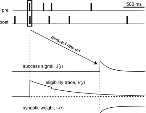
3.3 Illustration of learning by reward-modulated STDP. . . 38
4.1 Example of a stochastic neuron learning to map between an input spatio-temporal spike pattern and a target output spike train. . . 78
4.2 Performance comparison between two different stochastic neuron models when learning an increasing number of target output spikes. 79 4.3 Output spike rasters of two different stochastic neuron models when learning a target spike train containing 20 spikes. . . 80
5.1 Illustration of the time course of postsynaptic kernels used, and the resulting membrane potential of an SRM0 neuron. . . 90
5.2 Illustration of INST and FILT synaptic plasticity rules. . . 97
5.3 Dependence of synaptic weight change on the relative timing be-tween a target output spike and an input spike. . . 99 5.4 Dependence of reversal lag time sswitch on filter time constant τ
q,
5.5 Example of INST and FILT neurons learning to map between a single input-output spike pattern pair. . . 107 5.6 Synaptic weight distributions of INST and FILT neurons. . . 108 5.7 Network error as a function of the learning rate for INST, FILT
and CHRON neurons. . . 110
5.8 Performance of INST, FILT and CHRON neurons on a
classifica-tion task using precise temporal coding. . . 113
5.9 Comparative memory capacities of INST, FILT and CHRON
neu-rons as a function of their temporal encoding precision. . . 115 5.10 Performance of INST, FILT and CHRON neurons when learning
multiple target output spikes. . . 116 5.11 Illustration of learning paradigm based on Gaussian input noise. . 118 5.12 Performance of INST, FILT and CHRON neurons when classifying
noisy patterns. . . 119 6.1 Example of output layer weight update for MultilayerSpiker
learn-ing rule. . . 132 6.2 Example of hidden layer weight update for MultilayerSpiker. . . . 137
6.3 Example of MultilayerSpiker learning to map between an input
spike pattern and a target output spike train. . . 142 6.4 Evolution and final distribution of synaptic weights in a trained
multilayer network. . . 143 6.5 Robustness of MultilayerSpiker to input noise. . . 145 6.6 Learning the linearly non-separable exclusive-or (XOR) function
as a temporal code. . . 148 6.7 Performance of various network structures when learning mappings
of multiple input-output pattern pairs. . . 149 6.8 Performance of MultilayerSpiker on a classification task with fully
temporal coding. . . 152 6.9 Performance of MultilayerSpiker as applied to a noisy synthetic
dataset. . . 155 6.10 Learning a mapping between a spatio-temporal input-output spike
6.11 Dependence of performance on the network structure when learn-ing spatio-temporal spike pattern transformations. . . 159 6.12 Illustration of the bio-backprop learning rule: a biologically
in-spired implementation of spike-based backpropagation. . . 161 6.13 Performance of bio-backprop as a function of the number of input
Introduction
Spiking Neural Networks (SNNs) represent a third generation of artificial neural network models (Maass, 1997), conferring a substantial improvement with regard to the biological realism of neural simulations in comparison with previous gen-eration models. In particular, SNNs incorporate the time-domain as part of their operational model, such that spiking neurons constituting a network can commu-nicate with each other by transmitting pulsed signals or ‘spikes’ over time. In this way, an SNN is capable of encoding information by the precise timings of indi-vidual spikes, theoretically enabling superior computational power in comparison with a previous generation model such as a sigmoidal neural network (Maass, 1997).
Precise spike timing as a means to convey information in neural networks is biolog-ically supported (van Rullen et al., 2005) and is demonstrated to be advantageous over frequency-based codes by processing input features on a much shorter time-scale (Johansson & Birznieks, 2004; Gollisch & Meister, 2008). Moreover, the temporal precision by which individual spikes are reproduced can be very high: in some cases to within just one millisecond (Mainen & Sejnowski, 1995). For these reasons, much research attention is currently focused on the development of spike-based learning rules for SNNs, in order to more realistically model how learning and memory formation might take place in the nervous system. However, formulating effective learning rules that utilise a fully temporal code for SNNs is no small challenge owing to their inherent complexity.
settings, and work to train networks, through modifying the weights between neu-rons, to learn transformations between spatio-temporal input and desired output spike patterns (Kasinski & Ponulak, 2006); learning input-output transforma-tions is considered a generic processing task of biological neurons, and in most cases can straightforwardly be adapted to more specific learning tasks of interest. Currently, the majority of learning rules are restricted to just single-layer SNN structures: few rules are applicable to more complex SNN structures, for example those containing hidden layers of spiking neurons (G¨utig, 2014). Moreover, many spike-based learning rules lack analytical rigour in their formulation, meaning the optimality of their solutions cannot be guaranteed in general. Hence, in order to better realise the large potential in computational power offered by SNNs, it is desirable that a spike-based learning rule be proposed that is theoretically justifiable as well as versatile in its applicability.
This thesis aims to address the identified shortcomings of current learning rules for SNNs, by demonstrating that improved spike-based rules can not only be implemented in complex network structures but also provide optimal solutions when learning spike pattern transformations. Because of the significant role in-dividual spikes play in neural processing this thesis also places a strong emphasis on temporal coding as a part of SNN learning.
1.1
Objectives and Contributions
At present, few learning rules have been established for SNNs that are techni-cally efficient and yet versatile in their deployment. To take better advantage of the predicted high computational power of SNNs, it would be ideal to formulate general purpose learning rules that are applicable to various network structures and can convey information using the precise timings of spikes. Therefore, the overall aim of this thesis is to develop biologically-inspired learning rules for struc-tured SNNs that utilise spike-based encoding for the purpose of high performance neural computation.
The specific objectives of this thesis are summarised as follows:
learning rules, to explore the effect of single- and multi-spike based encod-ings on the accuracy of pattern recognition in SNNs.
• Formulate theoretically justified, spike-based learning rules for SNNs to ensure the optimality of resulting solutions are generally guaranteed.
• Formulate a more generalised spike-based learning rule that is applicable to structured SNNs containing hidden layers of spiking neurons, similar in concept to the backpropagation method as applied to rate-coded networks.
• Respect biological constraints of real neural networks, to support the use of derived spike-based learning rules as an explanatory model of neurobio-logical processing.
These objectives have led to several novel contributions, with resulting publica-tions listed at the end of this thesis. Each contribution is now briefly discussed in turn.
The first contribution is the application of an existing reward-modulated synaptic plasticity rule, specifically the Reward-maximisation (R-max) rule (Fr´emaux et al., 2010), to learning temporally precise sequences of output spikes by delayed reinforcement in an SNN. Our selection of the R-max rule is motivated by a desire for high biological realism in this initial work, and is inspired by emerging evi-dence suggesting that reward-modulated synaptic plasticity underlies behavioural learning in structures of the brain called the basal ganglia (Chakravarthy et al., 2010). This contribution is among the first to consider reinforcement-based learn-ing of large numbers of desired output spike times in an SNN, and introduces a new, effective method for this purpose (Gardner & Gr¨uning, 2013).
The second contribution is the formulation of two new supervised learning rules for training SNNs to transform between spatio-temporal input spike patterns and desired output spike trains. These learning rules are theoretically justified, and may be implemented online or offline depending on the level of biological realism that is desired. The performance of each rule is compared against that of the Chronotron: an existing supervised method which has previously been demonstrated to provide a very high network capacity in terms of the maximum number of input patterns that can be memorised (Florian, 2012).
The third contribution is the formulation of a new supervised multilayer learn-ing rule, termed MultilayerSpiker (Gardner et al., 2015), for feed-forward SNNs contain hidden layer spiking neurons. The rule generalises the probabilistic learn-ing method proposed by Pfister et al. (2006) from slearn-ingle-layer SNNs to multiple layers by combining a standard gradient ascent procedure with the method of backpropagation. MultilayerSpiker has strong theoretical justification, and works to modify synaptic weights in each layer of an SNN such that the likelihood of generating a desired spatio-temporal output spike pattern is maximised. The performance of the proposed learning rule is tested through several input-output spike pattern transformation tasks: both in terms of its final output accuracy and its convergence time. Finally, to better respect biological constraints of the actual nervous system, a biologically plausible implementation of the MultilayerSpiker rule is also proposed that mimics a reward-modulated learning paradigm.
1.2
Thesis Outline
The rest of this thesis is organised as follows.
Chapter 2provides background information on the biological neuron, including its information processing functionality as carried out via electrical signalling. This biological background is then used to inform descriptive mathematical mod-els of spiking neurons which constitute an SNN. Next, two main structural classes of SNNs are reviewed, including feed-forward and recurrent network structures. Finally, an overview is provided of two fundamental neural coding schemes used for neural computation: rate- and temporal-based coding.
Chapter 3 reviews two prominent synaptic plasticity mechanisms identified in the nervous system: Spike-Timing-Dependent Plasticity (STDP) and homeostatic plasticity. This is then followed by a review of biologically-inspired unsupervised, reinforcement and supervised learning methods that have been proposed for train-ing synapses in an SNN.
Chapter 4 presents a new reinforcement-based learning method for training SNNs to learn temporally precise sequences of output spikes in response to a spatio-temporal input pattern. This method is biologically plausible by
incor-porating delayed reward signals to guide synaptic plasticity, and by realistically simulating background noise during network learning.
Chapter 5 proposes two new supervised learning rules for performing efficient input-output spike pattern transformations in an SNN. The rules are extensively tested on a generic spike pattern classification task and benchmarked against an existing high-performance learning rule.
Chapter 6 introduces the new MultilayerSpiker learning rule for feed-forward SNNs containing hidden layer spiking neurons. The performance of the rule is tested by applying it to a variety of classification tasks, including measuring a trained SNN’s memory capacity as defined by the maximum number of input patterns it can learn to memorise. This chapter also proposes a more biologically plausible implementation of spike-based backpropagation.
Chapter 7provides the concluding remarks of this thesis, and discusses promis-ing directions for future research.
Spiking Neurons
The human central nervous system contains on the order of 1011 neurons which together form up to 1015 synaptic connections, and is responsible for directing behaviour in response to received sensory information. Understanding how such stimulus-response associations relate to the functions of constitutive neurons is a major aim of theoretical neuroscience, and has motivated the concept of a spiking neuron as an idealised model of a biological neuron.
This chapter begins by providing an overview of the biological neuron as found in the nervous system, with respect to its information processing capabilities via electrical signalling. This biological background is then used to form the basis of mathematical models for spiking neurons which transmit information via electri-cal pulses or ‘spikes’. Next, two main Spiking Neural Network (SNN) architec-tures are discussed: those containing layers of spiking neuron that are connected in a feed-forward manner, and those that contain a ‘reservoir’ of spiking neurons with recurrent connections. Finally, the topic of neural coding is examined which seeks to elucidate the relationship between stimulus and neuronal response.
2.1
Biological Background
The nervous system consists of two fundamental cell types: neurons and glial cells, with glial cells existing in a much greater abundance than neurons (Kandel et al., 2000). Currently, glial cells are understood to act mainly in a supportive
role, for example Schwann cells which aid neural signal transmission (Kandel et al., 2000), while neurons function as the primary information processing units in the nervous system (Trappenberg, 2010); despite this, it is noted that a certain subtype of glial cell, termed astrocytes, could play a more direct role in informa-tion processing than previously thought (Perea et al., 2009). For the purposes of this thesis, however, only information processing carried out by neuronal networks is considered.
2.1.1
Neuron Structure
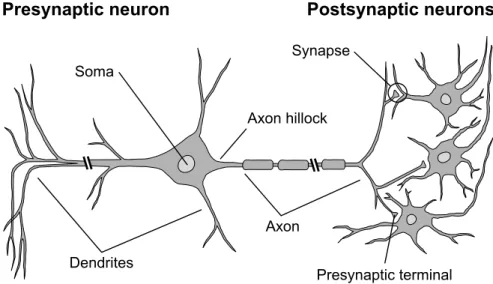
The structure of a typical neuron consists of four well-defined regions: the soma, dendrites, axon and presynaptic terminals (schematic shown in Fig. 2.1). The soma is the cell body, and is the metabolic center of the neuron; it contains the nucleus, as well as the cellular apparatus necessary for the maintenance of its structure and the execution of its functions (Kandel et al., 2000). The den-drites are cellular extensions which branch out, analogously to a tree, to receive incoming signals from other neurons. The axon extends away from the soma, appearing as a long tube-like structure, and in contrast with dendritestransmits signals generated by the neuron to other neighbouring neurons. Towards its end, the axon divides into several smaller branches which come into contact with the dendrites (or sometimes soma) of other neurons. These points of contact are termedsynapses and consist of a presynaptic cell which transmits a signal, and a postsynaptic cell which receives the signal; it is at these points where the ter-minates in what are called presynaptic terminals, allowing for the transmission of information from one neuron to the next. A postsynaptic neuron typically receives signals from a large number of presynaptic neurons, often having on the order of 104 synaptic connections in the vertebrate cortex (Kandel et al., 2000).
2.1.2
Electrical Signalling
Neurons communicate information via electrical signals, appearing as short elec-trical pulses with an amplitude close to 100 mV and lasting 1–2 ms in duration (Gerstner & Kistler, 2002). These brief electrical pulses, also commonly referred to as action potentials or spikes, typically appear similar in form: implying that
Axon
Presynaptic neuron Postsynaptic neurons
Presynaptic terminal Synapse
Soma
Dendrites
Axon hillock
Figure 2.1: Schematic of neuron structure and connectivity, as is typically found in the vertebrate cortex. Adapted from Fig. 2.1 in Trappenberg (2010).
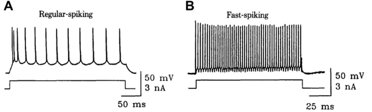
information is encoded not in their precise shape, but rather in the frequency with which they are generated or their precise timings. In this way, the spike is considered the fundamental unit of signal transmission in the brain (Gerstner & Kistler, 2002). Shown in Fig. 2.2 are example sequences of spikes, or spike trains, found in typical neocortical neurons.
In order to support the generation of action potentials a neuron must be elec-trically polarised, necessitating the maintenance of a certain potential difference across its cellular membrane. This potential difference, or membrane potential, is maintained by controlling the concentration gradients of various ions across the neuron’s membrane, and is achieved by the actions of ion channels that are embedded in the cellular membrane. Examples of ionic elements in the nervous system include sodium (Na+), potassium (K+), calcium (Ca2+) and chloride (Cl−
) (Trappenberg, 2010). Several types of ion channel exist, with varying levels of biophysical complexity, but in general they all share a common purpose: which is to regulate the passage of ions entering or exiting a neuron to control the mem-brane potential (Trappenberg, 2010). When a neuron is unstimulated its resting potential is typically measured at around−70 mV inside the cellular membrane, relative to its external environment (Dayan & Abbott, 2001).
When a neuron’s membrane potential increases above a certain threshold level, usually around 10 mV above its resting potential, a positive feedback process is
A
B
Figure 2.2: Example firing patterns of two types of neocortical neuron: regular-spiking and fast-regular-spiking. (A) In response to a constant current, a regular-regular-spiking neuron initially generates output spikes with high frequency which eventually be-come more widely spaced out. (B) A fast-spiking neuron has a much higher firing rate than that of (A) in response to the same current stimulus. Regular-spiking behaviour is most commonly found in electrophysiological studies. Regular-spiking neurons are excitatory, such that they work to induce postsynaptic spik-ing, while fast-spiking neurons are of an ihibitory nature, and supress postsynaptic activity. Reproduced from Fig. 1 in Connors & Gutnick (1990).
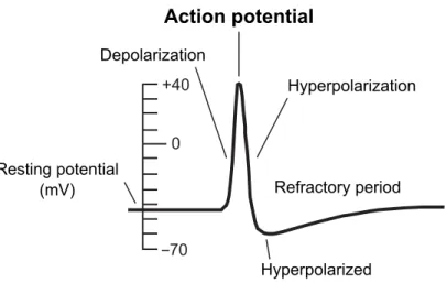
initiated and an action potential results. The time course of such an action po-tential can be characterised by three distinct phases: the rising phase, the falling phase and the undershoot phase. In the rising phase, the membrane potential rapidly increases to become more positively valued (depolarization). Once the membrane potential has peaked the falling phase follows, that is a sharp decrease in the potential to a (usually) more negative value (hyperpolarization). During the undershoot phase, the membrane potential temporarily drops beneath its usual resting potential (hyperpolarized), from where it then slowly returns to its resting value. This final phase also coincides with the refractory period: a time period lasting around 10 ms in which a subsequent action potential is impossible / difficult to initiate (Trappenberg, 2010). Fig. 2.3 illustrates the time course of a typical action potential.
Action potentials originate at a trigger site called theaxon hillock, or initial seg-ment of the axon (see Fig. 2.1); it is from here that they propagate away from the soma and along the axon at speeds ranging from between 1 and 100 m/s (Kandel et al., 2000). Moreover, the speed of action potential propagation is boosted by the presence of a myelin sheath, which envelopes most axons in the nervous system and works to prevent signal loss by acting as an insulating layer.
+40 70 0 Depolarization Action potential Hyperpolarization Refractory period Resting potential (mV) Hyperpolarized
Figure 2.3: The time course of a typical action potential, illustrating the rapid change in form over just a few milliseconds. Adapted from Fig. 2.6 in Trappenberg (2010).
Action potentials propagating along myelinated axons essentially ‘hop’ between nodes of Ranvier, or brief unmyelinated segments of an axon for signal regenera-tion, in a process called ‘saltatory conduction’ (Kandel et al., 2000). In this way, the amplitude of a travelling action potential is maintained at a constant value, thereby allowing it to travel over large distances without attenuation (Dayan & Abbott, 2001). Myelination of neuron axons is supported by certain subtypes of glial cell: Schwann cells in the peripheral nervous system, and oligodendrocytes in the central nervous system (Kandel et al., 2000).
2.1.3
Synapses and Chemical Signalling
Synapses are the interfaces between neurons, enabling the transfer of information from one neuron to the next, and are located at the points of contact between presynaptic axon terminals and postsynaptic dendrites and soma. There are two main types of synapse: chemical and electrical, although in the vertebrate brain the chemical synapse is most common (Gerstner & Kistler, 2002). The chemical synapse allows for the unidirectional propagation of an action potential from the presynaptic terminal to the postsynaptic dendrite, whereas the electrical synapse is bidirectional and allows action potentials to be transmitted both ways (Kandel et al., 2000). Relatively little is known about the functional consequences of electrical synapses, although they might be involved in the synchronization of
+ + + + + + + + + + + + + + + + + + + + + + + + + + + + + + + + ++ + + + + + Ligand-gated ion channel Synaptic vesicle Neurotransmitters Presynaptic terminal Postsynaptic dendrite
Figure 2.4: Schematic of a chemical synapse. Adapted from Fig. 2.3 in Trap-penberg (2010).
neurons (Gerstner & Kistler, 2002). Therefore, the attention of this thesis is restricted to the dynamics of just chemical synapses.
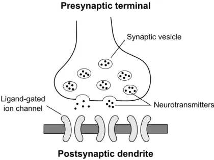
Shown in Fig. 2.4 is a schematic of a chemical synapse, consisting of a presynaptic terminal and receiving sites on a postsynaptic dendrite. In the presynaptic termi-nal, chemical substances called neurotransmitters are synthesised and stored in synaptic vesicles. Upon the arrival of an action potential a cascade of biochemical events are triggered, culminating in the release of the stored neurotransmitters into the synaptic cleft, that is the gap between the presynaptic terminal and postsynaptic dendrite; the size of this gap is very small, measuring only a few micrometers in distance between the pre- and postsynaptic membranes. Once released into the synaptic cleft the neurotransmitters diffuse across to the other side, binding to receptor sites on specialised (ligand-gated) ion channels embed-ded within the membrane of the postsynaptic dendrite. As a result, these ion channels allow an influx of ions from the surrounding extracellular fluid, leading to a graded change in membrane potential of the postsynaptic neuron. The re-sponse of the postsynaptic membrane potential to a presynaptic action potential is commonly referred to as the Postsynaptic Potential (PSP).
A wide variety of neurotransmitters are present in the nervous system. Com-mon examples include small biomolecules such as glutamate (Glu) or
gamma-aminobutyric acid (GABA) (Trappenberg, 2010). Beyond neurotransmitters, an-other class of chemical messenger is identifiable: neuromodulators, which act in a more global manner by being able to influence multiple synapses belonging to large groups of neurons. An important example of a neuromodulator is dopamine (DA), which is involved in neural circuits relating to motivation, attention and goal-directed behaviour (Schultz et al., 1997).
The response of a postsynaptic membrane potential to a presynaptic action poten-tial differs depending on the species of neurotransmitter received at its synapse. In the case of ion channels gated by Glu, the postsynaptic membrane potential responds with a positive increase, hence this synapse is an excitatory one. The response itself is referred to as an Excitatory Postsynaptic Potential (EPSP). By contrast, a synapse with postsynaptic ion channels gated by GABA are of an inhibitory nature, and effectively counteracts responses in the postsynaptic mem-brane potential triggered via excitatory synapses; this type of response is termed an Inhibitory Postsynaptic Potential (IPSP) (Trappenberg, 2010). Interestingly, the neuromodulator DA has several receptor subtypes, allowing it to effect ei-ther excitatory or inhibitory responses depending on the synaptic site at which it becomes available (Frank & Claus, 2006). As mentioned previously, there exist many types of chemical transmitter present in the nervous system, capable of elic-iting excitatory or inhibitory responses; the examples provided here are far from exhaustive, and just indicate at the enormous complexity of synaptic processing carried out by the nervous system. However, the fundamental mechanisms by which the biological synapse operates have been established, which shall be used in the next section to form the basis for mathematical modelling.
2.2
Spiking Neuron Models
Broadly speaking there exist three generations of artificial neuron model which constitute the computational units of a neural network, each aiming to replicate the essential functions of biological neurons in the nervous system (Maass, 1997). The first generation model is based on the McCulloch-Pitts neuron, which has since been developed into the more familiar perceptron (Minsky & Papert, 1987). Highly successful learning rules have been developed for perceptrons, and
impor-tantly have been extended to multilayer network structures, which are capable of generating any Boolean function subject to a sufficient number of hidden layer neurons (Bishop, 1995). Perceptrons mimic their biological counterparts in the sense that they take in a weighted input vector (synaptic scaling of input signals at dendrites) to then be equally summed over (as performed at the soma). The result of this summation is then thresholded to provide a binary output, using a step function as the neuron’s activation function (analogous to the functions of the axon hillock). Despite this, and unlike real neurons, perceptrons neglect the time domain, and are therefore restricted to processing inputs and producing binary outputs in an iterative manner.
The second generation neuron model instead uses a smoothed “activation func-tion” to transform a weighted sum of inputs to a continuous set of possible output values, using for example a sigmoid function to transform between analog input and output signals (Maass, 1997). Importantly, sigmoidal networks containing hidden layer neurons are universal approximators, as applied to continuous func-tions (Hornik, 1991). Characteristic of second generation models are their support for gradient descent based procedures, such as backpropagation for multilayer learning. From a biological perspective (Maass, 1997), second generation models can be seen to emulate neuronal rate coding, and in this sense can be consid-ered more biologically plausible than first generation models. However, such an implementation requires a relatively long time period in order to reliably sample the firing rate of a neuron; by comparison, the mammalian cortex is capable of rapidly processing visual stimuli in just under 100 ms (S. J. Thorpe & Imbert, 1989).
Spiking neurons are the third generation neuron model, improving largely on the biological realism of its predecessors through its incorporation of the precise timings of individual spikes. In this way, they offer the greatest potential for insight into the information processing capabilities of neural circuits in the ner-vous system. Furthermore, an SNN is theoretically predicted to be at least as computationally powerful as a previous generation neural network model when utilising a temporal code, and yet requiring less spiking neurons as its computa-tional units (Maass, 1997); in particular, their usage of a temporal code is widely considered to allow for much faster processing time of briefly presented stimuli (van Rullen et al., 2005). Despite these important advantages, spiking neurons
are somewhat more complex in their mathematical description, to the extent that there is a current lack of learning rules for SNNs that are as general domain as backpropagation algorithms are for rate-coded networks. It is the intention of this thesis to address this identified shortcoming, by proposing new learning methods for SNNs that are increasingly versatile in terms of their application while still taking advantage of their temporal processing capability.
This section now turns to reviewing implementations of spiking neuron models which provide a suitable trade-off between high biological realism and analytical tractability. These models shall then form the basis of our theoretical analysis of spike-based learning rules in the contribution chapters of this thesis.
2.2.1
Leaky Integrate-and-Fire (LIF) Model
The Leaky Integrate-and-Fire (LIF) neuron is one of the most commonly used spiking neuron models in computational neuroscience, owing to its relative sim-plicity and ease of analytical treatment. In all cases, LIF neurons are stimulated by either an external current or synaptic input from presynaptic neurons, and a characteristic threshold is used to define their output responses.
If we consider a single neuron, indexed byi, with a membrane potential ui(t) at
timet, then its subthreshold dynamics can be expressed by a differential equation:
τm
dui(t)
dt =−ui(t) +R Ii(t), (2.1)
where the neuron’s resting membrane potential is zero, and τm and R are model
parameters. The parameter τm is the membrane time constant, relating to the
‘leakage’ of charge across the neuron’s membrane when it is not at rest, and R
is the effective membrane resistance. Eq. (2.1) is the standard form for a LIF neuron, which analogously describes an electrical circuit containing a resistor in parallel with a capacitor that is charged by an external currentIi(t) (Gerstner &
Kistler, 2002).
The LIF model avoids modelling the precise form of an action potential, and instead characterizes spikes based on just their firing time. Hence, if we usetfi to refer to thefth spike timing of a neuron i, then according to the LIF model the
emission of a spike is determined by a threshold criterion:
tfi : ui(tfi) = ϑ , (2.2)
where ϑ is the neuron’s firing threshold. Upon the emission of an output spike, the postsynaptic membrane potential is immediately reset to a new value:
lim
t→tfi,t>tfi
ui(t) = ur, (2.3)
whereur< ϑ. If desired, this reset can be sustained over a brief period: ui(t) =ur
for tfi < t ≤ tfi + ∆abs, where ∆abs is an absolute refractory period. For times
t > tfi + ∆abs the dynamics of the neuron is again defined by Eq. (2.1) until the next incidence of a threshold crossing.
In the context of this thesis, the external currentIiinjected into the postsynaptic
neuron is appropriately defined as a summation over currents contributed by each synapse, elicited by presynaptic spiking. This sum depends on the strengths of individual synapses, parametrised by a real valued synaptic weight value wij
between the jth presynaptic neuron. The response of a postsynaptic current to a presynaptic spike is modelled by the so called ‘alpha-function’, denoted by α, that is typically taken as an exponential decay with a time constant on the order of a few milliseconds (Trappenberg, 2010). Assuming synaptic responses are non-interacting, then the total current is simply a linear combination of the synaptic terms: Ii(t) = X j X f wijα(t−tfj), (2.4)
wheretfj refers to the fth spike timing of a presynaptic neuron j.
Modelling synaptic responses by Eq. (2.4) is computationally efficient, and is well suited to the formulation of learning rules through parameter optimization tech-niques such as by gradient descent. An alternative, more biologically motivated approach might instead model the observed probabilistic release of neurotrans-mitters from synaptic vesicles, termed stochastic synaptic transmission (Dayan & Abbott, 2001); however, such an increase in precision usually comes at the cost of computational speed, making large-scale network simulations less feasible.
2.2.2
Spike Response Model (SRM)
The Spike Response Model (SRM) is a generalisation of the LIF model, and notationally differs by instead expressing the neuron’s membrane potential at
time t in terms of an integral over the past. The generality of SRM comes
from its inclusion of refractoriness, which can be modelled when the membrane potential explicitly depends on previous output spike times.
The SRM describes the subthreshold evolution of a postsynaptic membrane po-tentialuiin response to presynaptic spikes. When a presynaptic spike is received,
ui is perturbed from its resting value of zero, after which it gradually returns to
rest. The PSP kernel describes the time course ofui in response to a
presynap-tic spike. If the presynappresynap-tic input is sufficient to drive ui to a firing threshold
ϑ, then an output spike is generated by the postsynaptic neuron. The reset ker-nel κ influences the behaviour of ui in response to an output spike, effectively
describing the afterpotential of the postsynaptic neuron. Hence, if we consider a postsynaptic neuron with a last output spike at time ˆti, then its membrane
potential at timet is defined by (Gerstner & Kistler, 2002):
ui(t) := X j wij X f (t−ˆti, t−t f j) +κ(t−ˆti), (2.5)
where all functions have a dependence on the time since a last output spike,t−ˆti.
The response functions are defined such that , κ→0 for (t−tfj),(t−tˆi)→ ∞. Unlike the LIF model discussed previously, the threshold is not necessarily fixed, and may be dynamically adjusted to alter the postsynaptic neuron’s spiking behaviour. For example, if an absolute refractory period is required, then ϑ
can temporarily be set to a large positive value over selected time intervals
tfi < t≤tfi + ∆abs (Gerstner & Kistler, 2002).
2.2.3
Escape Noise Model
The firing activity of a biological neuron is highly variable, and is attributable, at least in part, to the continual bombardment of spikes originating from the tens of thousands of presynaptic connections it typically receives. This source of
background noise, referred to as ‘stochastic spike arrival’, is unlikely to be purely ‘nuisance noise’ that hampers neural processing in the nervous system; instead, it is more plausible that such background activity actually conveys meaningful signals processed by different neural pathways (Faisal et al., 2008). This idea relates to the massively-parallel processing nature of the brain, that must deal with continuous, overlapping streams of information transmitted by a variety of different sources. However, with respect to individual neuron modelling, it is impractical to consider such large-scale dynamics for driving variable spiking activity. A more practical, phenomenological approach would instead introduce randomly generated noise as part of a model to mimic the observed variability of biological neurons.
There are a number of approaches to including noise in a spiking neuron model: a key example is the escape noise model defined in Gerstner & Kistler (2002). Escape noise assumes a ‘noisy threshold’ for a neuron, such that the neuron’s firing threshold effectively fluctuates about some reference value as a result of random background activity. In this way, an output spike may be generated by an escape noise neuron even when its membrane potential is below the formal firing thresholdϑ. This idea is formalised by defining a probability densityρ for distributing output spikes, that has a functional dependence on the momentary distance between the neuron’s (noiseless) membrane potential and threshold:
ρ(t) = g(u(t)−ϑ), (2.6)
where u is defined by either the LIF model or SRM (see Eqs. (2.1) and (2.5), respectively). An illustration of this process is shown in Fig. 2.5. The arbitrary functiong is the ‘escape rate’, similar to that used to describe chemical reaction processes (van Kampen, 1992), and ideally is defined such thatg →0 foru→ −∞
(Gerstner & Kistler, 2002). The probability density ρ, also referred to as the stochastic intensity, is the likelihood of generating an output spike per unit time, and is interpreted as the neuron’s instantaneous firing density. The probability of generating an output spike at time t is given by
Prtf ∈[t, t+δt] = 1−exp (−δt ρ(t)) . (2.7)
Figure 2.5: Illustration of the escape noise model for probabilistically generating
neural spikes. A neuron with membrane potential u can fire at time t with
probability densityρ(t) =g(u(t)−ϑ), even if its formal firing thresholdϑ hasn’t been reached. The neuron’s last spike time is denoted by ˆt. Reproduced from Fig. 5.5 in Gerstner & Kistler (2002).
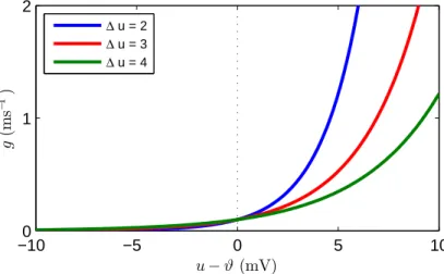
A variety of choices are available to define the escape rate functiong. A common selection is to take an exponential dependence:
g(u(t)−ϑ) =ρ0exp u(t)−ϑ ∆u , (2.8)
whereρ0 is the instantaneous firing density at threshold, and ∆u is a parameter which determines the ‘smoothness’ of the threshold. Interestingly, for suitable parameter choices of ρ0 and ∆u, Eq. (2.8) has been shown to well approximate the variable firing activity of neurons as recorded in vivo (Jolivet et al., 2006). An example of the exponential escape rate function defined by Eq. (2.8) is shown in Fig. 2.6.
Owing to its relative simplicity, the escape noise neuron represents an ideal choice for simulating background noise during simulations. Beyond its application as a stochastic spike generator, the escape noise model is also well suited to theoret-ical analysis by establishing a smooth functional dependence of output activity on internal network parameters; this shall become more apparent in subsequent chapters when escape noise is applied to formulating learning rules for SNNs. Finally, it is worth mentioning that although background noise can clearly be detrimental to neural processing, such as through signal degradation or by
jit-−100 −5 0 5 10 1 2 u−ϑ(mV) g (m s − 1 ) ∆ u = 2 ∆ u = 3 ∆ u = 4
Figure 2.6: Example of an escape rate with exponential dependence (see
Eq. (2.8)). The instantaneous firing density ρ = g(u−ϑ) rises exponentially with increasing u. Different colour curves correspond to different choices of the threshold parameter ∆u; larger ∆uresults in a ‘smoother’ firing threshold, result-ing in more variable output spikresult-ing. The rate at threshold is set toρ0 = 0.1 ms−1.
tering the timings of spikes, there can also be certain benefits. For example, stochastic resonance emerges as a phenomenon by which otherwise subthreshold input signals can be boosted by intermediate levels of noise to transmit meaning-ful information (Gerstner & Kistler, 2002).
2.2.4
Further Related Models
The LIF model and SRM represent just two possible choices for determining a postsynaptic neuron’s membrane potential. Other well-known models include the Izhikevich neuron (Izhikevich, 2003), the theta-neuron (or Ermentrout-Kopell canonical model) (Ermentrout & Kopell, 1986) and the Hodgkin-Huxley model (Dayan & Abbott, 2001). The Izhikevich neuron is defined by a two-dimensional system of differential equations, and is capable of reproducing the firing pat-terns of all known types of cortical neuron (Izhikevich, 2004). This model is computationally efficient, and as such is well suited for simulating the dynamics of large-scale networks of neurons with good biological plausibility (Izhikevich, 2006). By contrast, the theta-neuron is more simply defined by a one-dimensional differential equation, which depends on a single state variable. Also, given its non-linearity, a theta-neuron is still capable of exhibiting bursting behaviour unlike
the linear LIF model. Finally, the Hodgkin-Huxley model can exhibit most known behaviours of cortical neurons, and is also the most biophysically meaningful neu-ron model (Dayan & Abbott, 2001). The disadvantage of this model, however, is its computational complexity, requiring around 240 times more floating point operations than the LIF model (Izhikevich, 2004).
2.3
Spiking Network Structures
There exist a large number of different ways in which spiking neurons constitut-ing a neural network can be organised in terms of their connectivity. Broadly speaking, however, the structure of an SNN can be categorised into one of two main types: that of a feed-forward nature, where neural signals propagate in one direction only, and the other recurrent, which allows signals to propagate in both directions for more dynamical behaviour. This section briefly reviews each type in turn.
2.3.1
Feed-Forward Networks
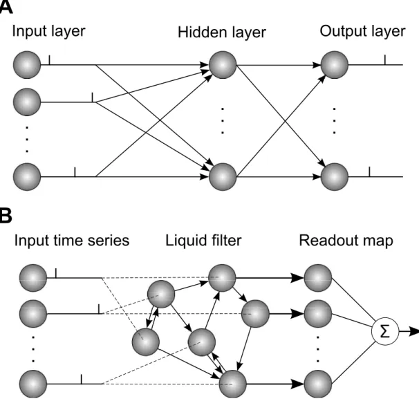
The simplest type of network has a feed-forward structure, where layers of neurons forwardly connect with those in subsequent layers. In the standard architecture of a feed-forward network there exists a single input and output layer, which presents input patterns to the network and determines its output responses, respectively (Trappenberg, 2010). Additional to this there can exist any number of intermedi-ate layers between the input and output layers, which contain hidden neurons. As mentioned in the previous section, the technique of backpropagation has demon-strated large success in training multilayer networks containing layers of hidden, rate-based neurons; in particular, multilayer networks can approximate any con-tinuous function to arbitrary precision for a suitable choice of neural activation function (Hornik, 1991). An illustration of a typical feed-forward multilayer SNN architecture is shown in Fig. 2.7A.
Input layer
Hidden layer
Output layer
. .
.
. .
.
. .
.
A
. .
.
Input time series
Liquid filter
Readout map
. .
.
B
Figure 2.7: Illustration of example SNN structures and their operation. (A) Feed-forward structure: neurons in the input layer are fully connected to neurons in the hidden layer, which in turn project to readout neurons in the output layer. Input layer neurons perform the task of presenting spatio-temporal spike patterns to the network, to be processed by neurons in downstream layers. Typically, the task of the network is to learn to map between spatio-temporal input and out-put spike patterns by optimising synaptic weights between neuron layers. (B) Recurrent reservoir: input neurons transmit time series data (spike trains) to a random subset of recurrently-connected reservoir neurons. These reservoir neu-rons act as a liquid filter: mapping the input data to a higher dimensional space to increase the separation between input classes. The output activity of reser-voir neurons is transmitted to a group of readout neurons, which determine the network’s response to the input data. Readout synapses are trained to produce desired network responses.
2.3.2
Recurrent Networks
Neural networks with recurrent connections exhibit more complex, dynamical behaviour than those with feed-forward connections, allowing for an internal, transient memory of input patterns that have previously been presented to the network. This behaviour emerges from the propagation of signals in both di-rections of the network, resulting from loops that are formed by the connections between neurons. An important example of a computing paradigm that takes ad-vantage of this dynamical property is reservoir computing (Jaeger, 2001; Maass et al., 2002; Chrol-Cannon & Jin, 2014), which works by transforming sequential input data into a state of dynamic activity within a ‘reservoir’ of recurrently-connected neurons. This reservoir of neurons periodically transmits its output activity to a module of readout neurons which, by gradient descent, have their weights trained to associate the input data with a desired network response. The spiking neuron variant for reservoir computing is referred to as a Liquid State Machine (LSM), which is capable of efficiently performing real-time com-putations on a time-varying input signal (see Fig. 2.7B) (Maass et al., 2002). An interesting observation by the authors of this study relates to the fading memory property of the system, or more specifically the ability of recurrently connected spiking neurons to remember the history of presented input data, as reflected in their output firing activity, that extends well beyond their short-term integration time constantτm. This memory property is considered to be essential for the
sys-tem’s success in making inferences about time series input data with regards to its long-term temporal evolution. However, despite their potential for increased computational power, the neural dynamics in an LSMs is significantly more com-plex to analyse than that in a simpler feed-forward SNN structure, making the formulation of spike-based learning methods for them much less straightforward.
2.4
Neural Coding
Neurons are characterised by their ability to rapidly transmit electrical signals over large distances in the body, and it is by this mechanism that neurons are able to transform sensory inputs into appropriate motor actions. The relationship
between stimulus and individual or ensemble neuronal responses is referred to as the neural code, and one of the fundamental aims of neuroscience is to decipher this code.
At present, two distinct hypotheses exist to explain the underlying nature of neural processing: the first based on a rate code, the second a temporal code. With respect to a rate code, the firing rate of a neuron is considered to fully describe a stimulus, whereas a temporal code instead uses the timings of neuronal spikes. Temporal coding is somewhat broad in its definition, and can refer, for example, to a coding scheme that relies on the precise timings of individual output spikes, or to a code that relies on the order in which first-spikes are generated over ensembles of output neurons (commonly referred to as rank-order coding (S. Thorpe et al., 2001)). This section briefly reviews each of the aforementioned coding schemes in turn, as well as their supporting experimental evidence.
2.4.1
Rate Coding
The idea that information pertaining to a stimulus is encoded in the firing rate of a neuron dates back to experiments performed by Adrian (1926) on the frog muscle, where the firing rate of stretch receptor neurons in the muscle depends on the force applied to them. Since then, rate coding has gained popularity as a mechanistic explanation for sensory processing in other areas of the nervous system, for example to describe the response of primary visual cortex neurons to a moving light stimulus (Henry et al., 1974).
In practice there exist several different definitions of a rate code, each depend-ing on how the firdepend-ing rate is calculated. The difference arises from the choice of averaging procedure used, such as by taking a temporal, repeated-trial or neuronal-ensemble average. A temporal average is defined as the neuronal spike count over some specified durationT divided by T, whereas a repeated-trial av-erage instead sums binned spike counts over several, identical experimental runs (trials) divided by the number of trials. A neuronal-ensemble average is defined similarly to a repeated trial average, but differs by instead averaging binned spike counts over large numbers of homogeneous neurons (Gerstner & Kistler, 2002). In most cases a simple temporal average is selected to define the firing rate,
al-though its usage can be restrictive: in order to reliably estimate the firing rate of a neuron a sufficiently long period of time must first elapse.
2.4.2
Temporal Coding
It is becoming increasingly clear that the relative timings of spikes transmitted by neurons, and not just their firing rates, are used to convey information regarding the features of input stimuli (van Rullen et al., 2005). Hence, the concept of a temporal code that is based on the timings of individual spikes becomes relevant. In many cases, a temporal code is identified by a high-frequency, rapidly fluctu-ating firing rate (Dayan & Abbott, 2001), or by the sensitivity of a postsynaptic neuron to the relative timings of presynaptic spikes: commonly referred to as coincidence detection (deCharms & Merzenich, 1996).
Spike timing as an encoding mechanism is advantageous over rate-based codes in the sense that it is capable of tracking rapidly changing input features, for example briefly presented images projected onto the retina (Gollisch & Meister, 2008), or tactile events signalled by the fingertip during object manipulations (Johansson & Birznieks, 2004). It is also apparent that spikes are generated with high temporal precision, typically on the order of a few milliseconds under variable conditions (Mainen & Sejnowski, 1995; Reich et al., 1997; Uzzell & Chichilnisky, 2004).
Precisely Timed Spikes. A possible application of a temporal coding scheme is the identification of input features using the precise timings ofall output spikes, also referred to as a fully temporal code (Gr¨uning & Bohte, 2014). This represents the most general usage of a temporal code, since in this case every individual spike timing is put to use, and has the potential to allow for a very large number of unique pattern encodings to be performed by just a single neuron operating over a limited time frame. Moreover, if there exist spike trains distributed over groups of neurons that are time-locked with respect to each other, then these patterns are referred to as polychronous groups (Izhikevich, 2006).
Rank-Order Coding. A further possible use of a temporal code relies on the order in which multiple output neurons emit their first spike in response to an
input stimulus (S. Thorpe & Gautrais, 1998). This coding scheme is ideally suited to time critical tasks, for example when neurons are subject to strong temporal constraints and only have time to emit a single output spike in response to brief input stimuli (van Rullen et al., 2005).
In terms of its implementation, rank-order coding represents a middle ground between a relatively simplistic rate code and a more complex fully temporal code: a rank-order code makes use of spike timings, allows for increased information storage in comparison with an equivalent rate code, and is simpler to decode than a code that uses multiple, precisely timed spikes (S. Thorpe et al., 2001). Despite this, rank-order coding has less potential than a fully temporal code in terms of the maximum number of pattern encodings it can perform, and additionally relies on large ensembles of output neurons for similar processing capability.
2.5
Chapter Summary
This chapter has outlined the fundamental principles of neuronal processing in the nervous system: starting with an overview of the biological neuron and its functions, spiking neurons as a descriptive mathematical model, and a final review of different neuronal coding mechanisms used to represent sensory information. From a phenomenological perspective, the LIF model and SRM are sufficiently capable of recreating the essential functions of biological neurons, and are partic-ularly well suited when the action potentials generated by a neuron are formalised as ‘all-or-none’ spike events. Importantly, their relative simplicity in comparison with alternative methods lends their utility to theoretical investigations of ner-vous system processing. For example, the SRM neuron, combined with escape noise, allows for a great deal of flexibility regarding the formulation of spike-based learning rules, as shall become apparent in the next chapter where existing learning rules for SNNs are reviewed.
From the overview in section 2.3 on the main structural classes of SNNs, it follows that there exist some disadvantages in implementing LSMs over feed-forward networks, despite their potential for strong computational power. In particular, an LSM can only provide a limited understanding of how neural computation
is actually carried out in the nervous system, which arises from its increased complexity in comparison with a simpler network structure: it is much more challenging to develop learning algorithms for recurrent network structures than it is for feed-forward structures. For this reason, the focus of this thesis shall be directed towards examining networks that are structured, or in other words, those that are organised as feed-forward single- and multilayer network structures, rather than those that have recurrent connections.
As reviewed in section 2.4, the advantages of temporal- over rate-based coding are clear; for example, by using a temporal code it is possible to track a rapidly changing stimulus based on the precise timings of individual spikes, whereas a rate code must first sample the stimulus over a relatively long duration before any representation can be formed. For the purposes of this thesis, the focus shall be on the use of a fully temporal code that uses multiple, precisely timed output spikes for pattern recognition, rather than, for example, a rank-order code; the reason for this is to better realise the maximum potential of derived learning methods for SNNs. Is it important to stress, however, that temporal coding is not a universal mechanism by which information is processed in the nervous system. Despite this, spikes themselves certainly underlie both rate- and temporal-based codes, and so it would seem most appropriate to formulate new learning methods based on individual spikes, for the simple reason that it is easier to transform a spike-based learning rule into a frequency-based rule than vice-versa.
Learning in Spiking Neural
Networks
This chapter reviews key advances in the field of theoretical neuroscience in re-lation to the learning of precisely timed spikes for neural information processing. The first section of this chapter provides an overview of synaptic plasticity pro-cesses identified in biological neural networks: with an emphasis on the process of Spike-Timing-Dependent Plasticity (STDP) which has been found through in-vivo and in-vitro experiments to essentially function as an unsupervised learning rule. In the next section a brief review of unsupervised learning is provided, in-cluding its relation to STDP as applied to training SNNs to learn spatio-temporal spike patterns. The following section then examines reinforcement-based learning as a biologically plausible scheme for training SNNs to form specific stimulus-response associations through reward-modulated synaptic weight changes. The final section then reviews prominent supervised learning rules for SNNs, many of which utilise the timings of multiple and precisely timed output spikes as a means to form representations of spatio-temporal input patterns.
3.1
Synaptic Plasticity
Learning in the brain is widely considered to take place through persistent mod-ifications of synaptic strengths between neurons. A variety of synaptic processes
have been experimentally observed to drive such modifications, ranging from short to longer term plasticity changes (Abbott & Nelson, 2000; Morrison et al., 2008; Caporale & Dan, 2008; Roberts & Bell, 2002). In this section two prominent synaptic plasticity mechanisms in the nervous system are reviewed: STDP and homoeostatic plasticity.
3.1.1
Spike-Timing-Dependent Plasticity (STDP)
The process of STDP has been identified in many areas of the nervous system, and is believed to play a major part in neuronal organisation during development (Caporale & Dan, 2008). STDP describes a persistent change in the synaptic strength between a pair of connected neurons based on their relative firing times, which is typically effective for relative timing differences of less than a few tens of milliseconds. In most cases the direction of synaptic strength change depends on the order in which pre- and postsynaptic spikes occur, for example: an increase in the synaptic strength (potentiation) for pre- before a postsynaptic spike, and a decrease in the synaptic strength (depression) for pre- after a postsynaptic spike. This process can be viewed as a spike-based formulation of Hebbian’s postulate for learning in the nervous system: if a presynaptic neuron “repeatedly or persistently takes part in firing” a postsynaptic neuron, then an increase in the synaptic strength between will ensue (Hebb, 1949). Experimentally, synaptic plasticity in hippocampal and cortical neurons has been demonstrated to behave in this way (Bi & Poo, 1998; Sj¨ostr¨om et al., 2001).
STDP is mathematically formalised by first defining a presynaptic neuron’s spike train as a sum of Dirac-delta functions:
Xj(t) = X
f
δ(t−tfj), (3.1)
that is a function of a sequence of firing times tfj for thejth presynaptic neuron (Gerstner & Kistler, 2002). Theith postsynaptic neuron’s spike train is similarly defined by Yi(t). Hence, the change in the synaptic strength (or weight) wij
according to a model of STDP (Gerstner & Kistler, 2002) is defined by dwij(t) dt =F+(wij)Yi(t) Z ∞ 0 W+(s)Xj(t−s) ds +F−(wij)Xj(t) Z ∞ 0 W−(s)Yi(t−s) ds . (3.2)
The kernel W±(s) = A±exp(−s/τ±) describes the ‘learning window’ of STDP:
typically giving a positive weight change for a pre- before postsynaptic spike (W+), and a negative weight change for a pre- after postsynaptic spike (W−).
The parameters A± and τ± control the amplitude and time scale of the learning
window, respectively. Typical parameter selections are: A+ = −A− = 1, τ+ = 10 ms and τ− = 20 ms (Gerstner & Kistler, 2002).
The function F±(wij) signifies a dependence of STDP on the actual value of the
synaptic weight, and its functional consequence can be to ensure that weights changed through STDP stay bounded. A common form is given by a power law:
F+(wij) =η(1−wij)µ and
F−(wij) =η ϕ wijµ , (3.3)
where η is the learning rate, ϕ an asymmetry parameter and µ a non-negative exponent for determining the dependence of weight changes on the current value of wij (G¨utig et al., 2003).
Two distinct STDP weight update rules emerge based on the choice of µ in
Eq. (3.3): so-called ‘additive STDP’ for µ = 0, and ‘multiplicative STDP’ for
µ= 1 (G¨utig et al., 2003; Morrison et al., 2008). Additive STDP updates have no dependence of the current weight value, therefore it is necessary to clip any weights that wander outside of a predefined boundary. By contrast, multiplica-tive STDP updates ensure weights remain bounded between 0 < wij < 1. The
choice of µ influences the equilibrium distribution of weights during unsuper-vised learning, such that additive STDP forms a bimodal distribution of weights, and multiplicative STDP a unimodal distribution of weights (G¨utig et al., 2003). Additive STDP has a tendency for run-away behaviour, by driving weights to extremal values, whereas multiplicative STDP is more homoeostatic in nature. It is noted that a choice ofµ= 0.4 gives a best fit to experimental data in Bi & Poo
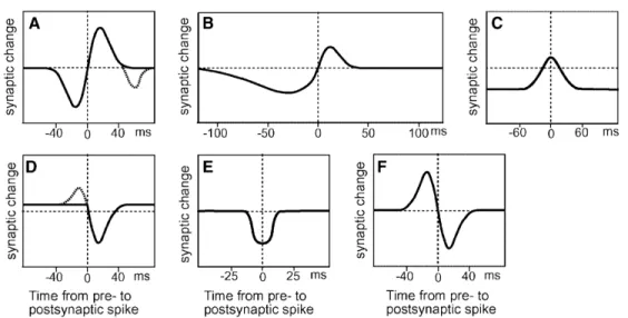
Figure 3.1: Examples of different Spike-Timing-Dependent Plasticity (STDP) rules identified in the nervous system, with synaptic change plotted as a function of the timing difference between a pre- and postsynaptic spike. Positive x-axis values indicate post- after presynaptic spikes. Panel A shows the classic, anti-symmetric Hebbian learning rule of STDP as found in hippocampal neurons (Bi & Poo, 1998). Panels B through F show several of the other forms STDP can take, including some that are non-localised in time. Figure adapted from Roberts & Bell (2002).
(1998), indicating a multiplicative dependence for STDP in biology (Morrison et al., 2007).
Although STDP is commonly assumed to behave in a Hebbian-like manner, there is no universal rule for explaining STDP throughout the entire nervous system. Experimental studies demonstrate STDP can take a variety of different forms, some even displaying anti-Hebbian learning (Roberts & Bell, 2002). Examples of STDP rules are shown in Fig. 3.1. The form of STDP described by Eq. (3.2) most closely approximates panel A.
The mechanisms of STDP discussed so far capture the essence of unsupervised learning in the brain, although it is by no means restricted to just the timings of coincident spikes; more recent studies have indicated at a further modulation of STDP by the postsynaptic, subthreshold membrane potential (Morrison et al., 2008). Such a level of detail is necessary when modelling experimental results obtained from multi-spike interactions in STDP (Clopath et al., 2010). Taken together, there can exist no ‘one-size fits all’ model for describing STDP, and the
selection of an appropriate model is highly conditional upon the problem under consideration.
3.1.2
Homeostatic Plasticity
Beyond STDP there exist further processes which contribute to synaptic plastic-ity in the nervous system. Homeostatic plasticplastic-ity is an important example, and in contrast with STDP acts in a regulatory role to maintain an optimal level of firing activity in neural circuits. For instance, synaptic scaling is a homeostatic plasticity mechanism which controls the firing activity of a neuron by multiplica-tively scaling (upwards or downwards) the synaptic strengths of all its afferent connections (Abbott & Nelson, 2000; Morrison et al., 2008). Interestingly, simula-tions of synaptic scaling in SNNs demonstrate an increase in competition between afferent synaptic connections; such competition is useful for influencing develop-mental processes, and to normalise output neuronal firing rates to minimise the impact of variable input activity on learning (van Rossum et al., 2000).
A simplified mathematical model of synaptic scaling, with respect to a postsy-naptic neuron i, is given by (van Rossum et al., 2000):
∆wij = ψ |wij|(νmax−νi) if νi > νmax ψ |wij|(νmin−νi) if νi < νmin, (3.4)
where ψ is the scaling strength, νi the actual output firing rate of the neuron,
andνmaxandνminthe maximum and minimum reference postsynaptic firing rates, respectively. The above drives the firing rate of the postsynaptic neuron to remain within the rangeνmin ≤νi ≤νmax by iteratively scaling weights, thereby making an SNN less sensitive to its initial state and preventing extremes in the firing activity of the neuron (Gr¨uning & Sporea, 2012; Sporea & Gr¨uning, 2013). Another form of homeostatic plasticity is synaptic redistribution, a short term plasticity process which regulates postsynaptic neuronal firing activity based on the probabilistic release of presynaptic transmitters into the synaptic cleft (Ab-bott & Nelson, 2000). A high presynaptic firing rate leads to a more rapid de-pletion in the amount of presynaptic transmitters available for release, which in turn decreases the postsynaptic firing rate. Probabilistic approaches to modelling
this process and its relation to neuronal dynamics are reviewed in Morrison et al. (2008). Beyond its regulation of neuronal firing activity, synaptic redistribution has also been investigated as a stochastic process for driving reinforcement-based learning in networks of spiking neurons (Seung, 2003).
There are a multitude of further synaptic plasticity processes in the brain that contribute to learning, although discussing each in turn is beyond the scope of this thesis. The key mechanisms underlying synaptic plasticity in the nervous system have been outlined, and the aim shall now be to relate these plasticity processes to the learning of spatio-temporal spike patterns in SNNs.
3.2
Unsupervised Learning
The process of unsupervised learning in neural networks refers to the adaptation of synapses to the statistics of pre- and postsynaptic neuronal activity. In this learning paradigm no task is explicitly specified that must be solved by the net-work: the network essentially learns by itself to form internal representations of particular input patterns, based on their overall statistical structure (Morrison et al., 2008). By this process, a network can be trained to cluster or classify input data through self-organisation (Bohte, Poutr´e, & Kok, 2002), for instance by adjusting synaptic weights via the correlation-based STDP rule as described previously. In this section, a learning method which uses STDP to train SNNs to form representations of spatio-temporal spike patterns is examined.
3.2.1
STDP-Based Spike Pattern Learning
An important example of unsupervised learning in SNNs has been proposed by (Masquelier et al., 2008), where STDP (see Eq. (3.2)) was applied to training a single postsynaptic neuron to detect a single, repeatedly presented, input spatio-temporal spike pattern embedded in random background spiking activity. Specif-ically, the network was of a feed-forward structure, containing a large number of presynaptic neurons that provided input to the postsynaptic ‘detector’ neuron. Half of the presynaptic neurons continuously