Exploiting Abstract Syntax Trees to Locate Software Defects

(1)

EXPLOITING ABSTRACT SYNTAX

TREES TO LOCATE SOFTWARE

DEFECTS

by

THOMAS JOSHUA SHIPPEY

Submitted to the University of Hertfordshire in partial fulfilment of the requirements of the degree of

DOCTOR OF PHILOSOPHY

School of Computer Sciences University of Hertfordshire

(2)

(3)

Acknowledgements

Who would have thought that an interval in a Vancouver Canucks NHL game would have led me to undertaking a PhD? Not me. 2am boredom led me to have a look at some code that created a digital clock. The Java clock had been developed by David Bowes earlier in the day. It had a alarm that let out a dull beep when a certain time had been reached. I thought, surely this can be improved? So it took me the next two periods of the Canucks game to modify the alarm clock so it played songs instead of a beep when the alarm was set off. Upon showing this to David, he seemed impressed. Ultimately, this led to David supervising my Masters project and the rest they say, is history. So, my first acknowledgement goes to my principal supervisor David Bowes. Without your encouragement and belief in me, I would not have started on this journey. You have been fantastic over the past three years (four if you include the Masters!). Your passion for the subject is infectious and your enthusiasm has compelled me to always want to impress you with new work each week. It has been a real pleasure to work with you over the course of this PhD.

My second acknowledgement goes to my other supervisors; Tracy Hall and Bruce Christianson. You both have been a huge support in the past three years. Tracy, thank you for helping me develop the rigour needed to undergo a PhD. I must thank you for being patient as my writing style went from bad, to ok, to acceptable, to good. I hope that I have finally figured it out and hopefully your red pen can have some well earned rest. Bruce, your experience and guidance has been invaluable and it has been a pleasure to work with you over the past few years. Thirdly, I would like to thank every-one that I have met in the STRI and Computer Science department for helping me through my PhD years. I would like to thank my mum, Ruth Shippey for everything that she has done for me over the last 28 years. Quite literally, without you I would not be in the position to do so well in life. Your support and guidance over the years has been amazing. You have created a great home and loving atmosphere that has allowed me to achieve what I have achieved so far. I know the last nine years have been hard, but you have been the rock I have been able to lean on, even when I know you are crumbling. You are the best mum I could have asked for, I hope you are proud of what I have achieved. I would like to thank my sister, Amy Shippey for all her support in the last couple of years. Thank you for being the annoying little sister that made me hide away in my room and therefore let me get my work done (only kidding!). Thank you to my other sister, Catherine. You only came in to my life during the PhD but I couldn’t ask for a better older sister. Your love and help has been invaluable. Thank you to all my friends and family, for all your help and understanding during the last three years. The laughs you provide have helped keep me going. Special mention has to go to the Bradford WhatsApp group for allowing me to vent when Arsenal and Arsene decide to ruin the weekend. I am going to have to think of a better excuse to bail out of events now that the PhD is over! Thank you Katie Steingold. Thank you for all your love, support and encouragement. Thank you for being there for me when I need it most. I hope I can repay you in the years to come.

Finally, I want to thank my dad, Phil Shippey. Unfortunately, you will not be around to see what I have achieved. There is not a day that goes by that I do not think of you. Without the love and support you gave to me, I would not be a man capable of completing a PhD thesis. You always said, you did not know how to be a good father as you did not have one yourself. You never had to worry about that, you were the best I could have ever asked for. Wherever you are, I do hope you are proud of me.

(4)

(5)

iii

ABSTRACT

Context. Software defect prediction aims to reduce the large costs involved with faults in a software system. A wide range of traditional software metrics have been evaluated as potential defect indicators. These traditional metrics are derived from the source code or from the software development process. Studies have shown that no metric clearly out performs another and identifying defect-prone code using traditional metrics has reached a performance ceiling. Less traditional metrics have been studied, with these metrics being derived from the natural language of the source code. These newer, less traditional and finer grained metrics have shown promise within defect prediction.

Aims. The aim of this dissertation is to study the relationship between short Java constructs and the faultiness of source code. To study this relationship this dissertation introduces the concept of a Javasequenceand Javacode snippet. Sequences are created by using the Java abstract syntax tree. The ordering of the nodes within the abstract syntax tree creates the sequences, while small subsequences of this sequence are the code snippets. The dissertation tries to find a relationship between the code snippets and faulty and non-faulty code. This dissertation also looks at the evolution of the code snippets as a system matures, to discover whether code snippets significantly associated with faulty code change over time.

Methods. To achieve the aims of the dissertation, two main techniques have been developed; finding defective code and extracting Java sequences and code snippets. Finding defective code has been split into two areas - finding the defect fix and defect insertion points. To find the defect fix points an implementation of the bug-linking algorithm has been developed, calledS+_e. Two algorithms were developed to extract the sequences and the code snippets. The code snippets are analysed using the binomial test to find which ones are significantly associated with faulty and non-faulty code. These techniques have been performed on five different Java datasets; ArgoUML, AspectJ and three releases of Eclipse.JDT.core

Results. There are significant associations between some code snippets and faulty code. Fre-quently occurring fault-prone code snippets include those associated with identifiers, method calls and variables. There are some code snippets significantly associated with faults that are always in faulty code. There are 201 code snippets that are snippets significantly associated with faults across all five of the systems. The technique is unable to find any significant associations between code snippets and non-faulty code. The relationship between code snippets and faults seems to change as the system evolves with more snippets becoming fault-prone as Eclipse.JDT.core evolved over the three releases analysed.

Conclusions. This dissertation has introduced the concept of code snippets into software engi-neering and defect prediction. The use of code snippets offers a promising approach to identifying potentially defective code. Unlike previous approaches, code snippets are based on a comprehensive analysis of low level code features and potentially allow the full set of code defects to be identified. Initial research into the relationship between code snippets and faults has shown that some code constructs or features are significantly related to software faults. The significant associations between code snippets and faults has provided additional empirical evidence to some already researched bad constructs within defect prediction. The code snippets have shown that some constructs significantly associated with faults are located in all five systems, and although this set is small finding any defect indicators that transfer successfully from one system to another is rare.

(6)

(7)

List of Figures

1.1 ADO_WHILE_LOOPwhich prints out the value of x while x is less than 20. Figure 1.2 shows the AST walkthrough for this piece of code and Figure 1.3 is the sequence this

code will make in AST kinds.. . . 4

1.2 This figure shows the AST walkthrough for theDO_WHILE_LOOPshown in Figure 1.1. The number on the line represents the order in which the tree is traversed. Figure 1.3 shows the sequence that this traversed tree will make. . . 4

1.3 The sequence of theDO_WHILE_LOOPin 1.1 and the traversed AST in 1.2 makes. . . 5

2.1 A diagram depicting the relationship between problems, failures, faults and defects. A fault is a subtype of a defect. A defect is a fault when the error manifests itself during software execution. Based on the diagram fromIEEE[2010] . . . 10

2.2 A bar chart showing the costs of defects within a software system at different stages of development. The costs rise due to the extra costs of fixing a defect at different stages of the development. Shown inPressman[2001]. . . 11

2.3 A diagram showing how defect prediction can be carried out. . . 12

2.4 A Defects’s ‘Life’- this timeline shows the life of a defect within a software system. The defect was introduced in March 2013 and is not fixed until a year later. During this time, the code that is affected by this defect is labeled as defective (the red line). . . 13

2.5 Examples of control graphs and their calculated complexity scores . . . 15

2.6 Inheritance between Swing classes in Java.. . . 17

2.7 The three node subgraphs examined byPetric and Grbac[2014]. . . 24

2.8 A example of a Southern Blot. Taken fromJeffreys et al.[1985] article in Nature . . . . 25

2.9 An interpretation of a southern blot for Java methods . . . 25

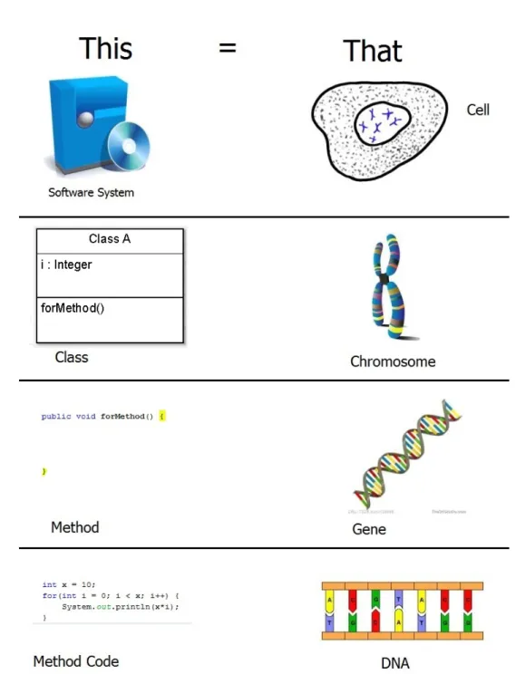
2.10 A graphic to show the software product to living organism analogy. In the first instance a software product/package is the cell in an living organism. These cells are made up of chromosomes, just like a software package is made up of classes. These chromosomes are made up of different genes, while a class is made up of different methods. Finally, the genes are sequences of DNA, like a method is made up of code. . . 27

3.1 de Groot and Spiekerman[1969]’s empirical methodological cycle. Taken from [Daan 2014] . . . 32

3.2 Overview of the process that will be undertaken within the PhD. . . 36

3.3 The correlation between the spending of science, space and technology in the US and the suicide by hanging, strangulation and suffocation rate in the US is 0.99. This is very high, but obviously the two are not causally linked. Taken fromSpuriousCorrelations [2014] . . . 41

4.1 A Venn Diagram to show the agreement between the three implementations.S+_e includes all but one bug-link of both the other two implementations. . . 51

4.2 A scatterplot to show how many lines change as a defect is fixed in each system studied. EJDT 3.0 has many more lines added or deleted per defect fix than the other systems. . . 54

(12)

5.2 The code from figure 5.1 transformed into aKindsequence. (A full list of the kinds and their meanings is located in Appendix A.) . . . 58 5.3 This figure shows the AST walkthrough for theforMethod shown in Figure 5.1. The

number on the line represents the order in which the tree is traversed.. . . 59 5.4 The possible set of 12 code snippets taken from an example method sequenceA; A;

C; D; E. . . 60 5.5 This figure shows how the sliding window algorithm extracts the code snippets from

the example method sequenceA; A; C; D; E. The right hand side shows the current position of the sliding window algorithm, while the left hand side shows the code snippet that has been extracted at that position. The right hand side is the complete set of possible code snippets that can be extracted from the example method sequence (when maximum code snippet length equals three).. . . 61 5.6 A scatterplot to show the high correlation between the LOC in a method and the number

of kinds in a sequence. The calculated correlation is 0.95 . . . 63 5.7 A vioplot to show the distribution of the sequence lengths in all five of the datasets

analysed. There are a high proportion of sequences that are very small, compared to those sequences that are very large. . . 64 5.8 A venn diagram to show how the unique snippets found in each dataset overlap with

each other. In total there are 35,214 code snippets that are found in all five datasets. . . . 65 6.1 A Venn diagram to show the distribution of associations between each of the studied

systems. In total 201 snippets are significantly associated with faults in all five of the systems. . . 71 6.2 The red portion of text is an example of the code snippet METHOD_INVOCATION;

MEMBER_SELECT; IDENTIFIER; MEMBER_SELECT; IDENTIFIER;

MEMBER_SELECT. This method was faulty in the EJDT 3.0 system in class JavadocRe-turnStatement.java. . . 72 6.3 A bar chart to show the percentage of significant snippets to non significant snippets at

each code snippet length. As the code snippet length increases, the chance of a typical code snippet of that length being significant decreases. . . 73 6.4 A bar chart to show the percentage of significant snippets to non significant snippets at

each code snippet length for each of the five systems. EJDT 3.1 and EJDT 3.0 code snippets with a length of one have the greatest chance of being snippets significantly associated with faults. . . 74 6.5 An example of two of two methods that are suspected to be code clones in

EJDT 2.0. The red text is code snippet IDENTIFIER; NEW_CLASS; IDENTIFIER; METHOD_INVOCATION; IDENTIFIER; RETURN. This code snippet appeared in all 52 defective methods. . . 77 6.6 A histogram to show how the majority of code snippets significantly associated with

faults are in a very small number of methods across the five systems analysed. 97% of the code snippets significantly associated with faults feature in 1,000 methods or less. 1,000 methods make up only 2% of the total methods in all of the systems. NB There are values in the far side of the x axis, however they are too small to be seen! . . . 78 6.7 The red portion of text is an example of the code snippet IF; PARENTHESIZED;

CONDITIONAL_AND. This method was faulty in the EJDT 3.1 system in class SourceEle-mentParser.java. This class extracts structural and reference information from a piece of source code. . . 81

(13)

List of Figures xi

6.8 The red portion of text is an example of the code snippet FOR_LOOP; VARIABLE; MODIFIERS; IDENTIFIER; METHOD_INVOCATION; MEMBER_SELECT; IDENTIFIER. This method was faulty in the AspectJ system in class AjLookupEnviron-ment. This class overrides the default Eclipse LookupEnvironAjLookupEnviron-ment.. . . 81 6.9 The red portion of text is an example of the code snippet EXPRESSION_STATEMENT;

METHOD_INVOCATION; MEMBER_SELECT; METHOD_INVOCATION. This method was faulty in the ArgoUML system in class TabTaggedValues.java. This class is table view of a UML models elements tagged values. . . 82 6.10 A Venn diagram to show the distribution of snippet associations between each of the

systems. . . 83 6.11 A Venn Diagram to show the association of snippets significantly associated with faulty

methods among the EJDT releases. Only 12% of snippets are significantly associated with faults in all three releases. . . 84

(14)

(15)

List of Tables

1.1 A table showing how the AST is traversed. Each part of the tree is broken down into parts as it goes through the code. The numbers correlate to the order in which it traverses

the tree shown in Figure 1.2. . . 5

2.1 Halstead complexity metrics created byHalstead[1977]. . . 16

2.2 Class level OO metrics described in the defect prediction literature [D’Ambros et al. 2010] 18 2.3 List of Change metrics used in theMoser et al.[2008] study. . . 20

2.4 The four churn metrics based on code blocks introduced byLayman et al.[2008] . . . . 22

3.1 The criteria for the binomial test [Garson 2004] and how the data used in this dissertation passes the criteria. . . 38

3.2 The criteria assessment for the three programs analysed in this dissertation. Each pro-gram is a mature open source propro-gram with a Git repository and a bug database. . . 42

3.3 The five systems analysed in this dissertation. . . 43

4.1 Kappa coefficients to show the level of agreement between the implementations. The proportion of agreement is very low for all datasets. . . 50

4.2 Number of commits in S+_e compared to Zimmermann et al. [2007] on the different branches. There does not seem to be a problem withZimmermann et al.[2007] missing branches. . . 52

4.3 Checking the bug-links for false positives. Zimmermann has similar precision but lower recall. . . 52

4.4 The five datasets analysed in this dataset.. . . 52

4.5 Total amount of Bug-Links for each dataset . . . 53

4.6 A table to show the changes when the defects are fixed in all datasets. . . 54

4.7 Table to show the defect density of each of the datasets. . . 54

5.1 Table to show the average length of the sequences in each of the five programs. Eclipse has a longer average sequence length than the other two programs. . . 62

5.2 The total amount of snippets in each of the systems investigated in this dissertation. . . . 64

6.1 Table to show the number of code snippets and significant code snippets for each pro-gram. EJDT 3.1 has the most code snippets significantly located in defective methods. . 69

6.2 The top five most frequently occurring snippets significantly associated with faults in each of the five systems. . . 70

6.3 The number of code snippets a single kind appears in the top 10% most frequently occurring code snippets significantly associated with faults across all five of the systems 70 6.4 Table to show the top five sub-snippets in the 195 snippets greater than length one that are significantly associated with faults in all five datasets. METHOD_INVOCATION;MEMBER_SELECTappears most frequently. . . 72

6.5 Table to show the percentage of code snippets that are always significantly associated with faults and the percentage of methods they appear in. Code snippets that are always significantly associated with faults appear in one to five methods 99% of the time. . . 75

(16)

6.6 All of the 29 code snippets that are significantly associated with faults and are always defective in EJDT 2.0. . . 76 6.7 Table to show the different method name types in the 118 methods that contain the 29

significant snippets that are always faulty. There are only four different method name types, which could indicate that the methods were faulty clones of each other. . . 77 6.8 Table to show the cumulative frequencies of the code snippets significantly associated

with faults and the number of methods they appear within. Just over 99% of the code snippets significantly associated with faults only feature in 3,000 methods or less. Only 380 of the possible 43,961 snippets appear in over 3,000 methods. . . 79 6.9 Table to show amount of code snippets that appear in the top 1% of methods in their

respective systems. All systems total does not equal the the five systems total as a different cut offpoint is used for all systems. . . 79 6.10 Table to show the top five most faulty significant snippets for each of the systems that

appear in the top 1% of methods ranked by percentage faulty. . . 80 6.11 Table to show the number of unique snippets significantly associated with non-faulty

se-quences. There are a lot fewer snippets associated with non-faulty sequences compared to faulty sequences. . . 81 A.1 The 92 Java Kinds located in the Tree.Kind and their descriptions . . . 123 A.2 The 201 code snippets that are significantly associated with faults across all five systems

(17)

C

hapter

1

Introduction

“They don’t make bugs like Bunny anymore.”

– Olav Mjelde

Defective software code is expensive for the software industry in terms of money, time, effort and loss of reputation. It has been estimated that around $312 billion per year is spent on finding and reducing the number of defects in software systems [Brady 2013]. Software faults can also effect a user’s confidence in a system or product, for example; the opening of the US Affordable Health Care Act website, which damaged the reputation of the Act and the US president [Connor 2013], or when Samsung had to pull an Android 4.3 software update for its Samsung S3 mobile product. The software update caused a number of problems, for example an increase in battery drain, applications not working and alarms not activating [BBC 2013].

Software defect prediction is an important area of research trying to identify defective software code. Early identification of defects1 may help reduce the costs caused by defects. This is because the costs associated with fixing defects increase as system maturity increases [Pressman 2001]. Defect prediction uses algorithms to create models which predict the areas of software code where defects are likely to occur. It is a well researched area, with over 200 studies published between 2000 and 2010 reporting software defect prediction models [Hall et al. 2012]. Despite software prediction being a well researched area, existing defect prediction models are thought to have reached a predictive performance ceiling [Menzies et al. 2010].

Software defect prediction models rely on independent and dependent variables. Independent variables are normally software metrics collected from software systems, for example software metrics include software code metrics (SCM) and process metrics. Examples of SCMs used in the models include Lines of Code (LOC) [Fenton and Ohlsson 2000,Mende and Koschke 2009,Weyuker et al. 2010,Zhou et al. 2010], object oriented metrics [Arisholm et al. 2010,Bird et al. 2009b,Cruz and Ochimizu 2009, D’Ambros et al. 2010,Khoshgoftaar et al. 2010] and complexity measures [Mende and Koschke 2010, Menzies et al. 2007,Turhan et al. 2009]. Process metrics include code churn [Hassan 2009, Khosh-goftaar et al. 1996, Nagappan et al. 2010,Nagappan and Ball 2005, Purushothaman and Perry 2005, ´Sliwerski et al. 2005], revision control histories [Bell et al. 2006,Graves et al. 2000,Hassan and Holt 2005,Moser et al. 2008,Ostrand et al. 2005,Weyuker et al. 2006] and number of previous faults identi-fied [Hassan and Holt 2005,Kim et al. 2007]. The dependent variables in the models are normally fault variables (e.g. the number of faults predicted in a module, or if a fault has been predicted in the module). Traditional SCM have been extensively used but most of the metrics introduced above suffer from being very coarse grained with capability to measure only a small sub-set of code features.Gray et al.[2011]

1_{The IEEE definition}_IEEE_[₂₀₁₀_{] of a fault being a reported defect, where a defect is a mistake in code made by a developer}

(18)

suggest that the coarse grained nature of such metrics prevents machine learning techniques from eff ec-tively differentiating between defective and non-defective modules: if one module has the same metric values as another (say in terms of LOC), but they have not been labelled the same in terms of their de-fectiveness, this will hinder the learning algorithm’s ability to learn. Gray et al.[2011] identifies many modules in the NASA datasets2which have identical values across a range of metrics but different de-fectiveness labels. This suggests that commonly used metrics are not sufficient to differentiate modules for defect prediction.

The natural language of software code has been used to identify defects. Natural language analysis is the study of the linguistic quality of the source code text. Poor language used by developers for creating code could harm the quality of the code and could hinder program comprehension [Abebe et al. 2012]. Program identifiers were investigated byAbebe et al.[2012] andBinkley et al.[2009] who both showed that the use of language processing measures were useful in defect prediction. Character analysis has also been used to associate text with defective modules [Zeller et al. 2011]. Detection using patterns of words in faulty modules was developed by Mizuno et al.[2007], where a fault-proneness filtering technique was developed based on spam filtering approaches. The use of text has problems due to differing languages spoken by different developers and the analysis of text has to have custom-made lexers to break it down into smaller pieces. This dissertation is interested in the the key building blocks of the source code, rather than the linguistic properties of the written code.

Defective code is not limited to software engineering. In biology, problems involving living organisms can be related to defective ‘code’. Scientists investigate genetic disorders (defects in the living organism) using chromosomes. A chromosome is“an organised package of DNA found in the nucleus of a cell” [Institute 2014]. Humans have 23 different pairs of chromosomes and these chromosomes were used to discover if the existence/non-existence of a certain chromosome was associated with a particular genetic disorder (e.g. Down Syndrome is an example in which three copies of a chromosome exist, instead of two ). This information could be used to predict whether a foetus or new born baby had a genetic disorder. Each chromosome is made up of DNA tightly coiled many times around proteins. It is this precise DNA sequence that allowed scientists to perform finer grained techniques to predict genetic disorders. DNA carries genetic information of living organisms [Insitute 2011]. The information is a sequence of four base pairs and this information is passed down from the parent organism to the child. The base pairs are the building blocks of the DNA and base pairs form between specific biological compounds called nucleobases. These base pairs are commonly known as adenine, guanine, thymine and cytosine and they are normally abbreviated to A, G, T and C. It is the order of the base pairs that determine the characteristics of a living organism (e.g. a sequence of TAAATGTCAA within a certain gene may indicate a person will have blue eyes). The greater the difference in the DNA sequence, the greater the difference in the organism. Small changes in the sequences that occur within the overall DNA sequence can be used to create a DNA profile. These DNA profiles can be used to identify correctly or incorrectly functioning genes within a living organism. Profiles are isolated and identified using chemical techniques, a process which produces a DNA fingerprint [Jeffreys et al. 1985]. Genes which do not work can be identified by comparing their profile (fingerprint) with that of a working gene. Although non functional genes may be due to small changes, the profiles can detect them. If we apply this analogy to software code, we can imagine that a small change to a piece of code could also impact on the correct functioning of that unit.

The aim of this dissertation is to develop an approach to identify features of software code, based on the principles of DNA profiling. This approach will create a new technique, by creating a profile based on

(19)

3

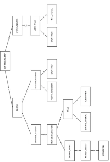
the subsequences of particular pieces of code. The approach is based on analysing the Abstract Syntax Tree (AST) for Java code. The nodes in a Java AST contain Java kinds. These Java kinds3 define the low level programming constructs that have been used in a piece of code and the order in which these are used. A method is turned into a sequence of kinds by walking its corresponding AST tree. The sequences are created by parsing the source code into an AST and then traversing the AST to gather the kind sequence. Figures1.1, 1.2 and1.3 and the Table 1.1 show how a piece of software code is transformed into a kind sequence. Figure1.1is a piece of code that describes aDo While Loopwhich prints of the value of xwhile the value is under 20. Figure1.2shows the AST which is created when this Do While Loop is parsed by the Java parser. Each white rectangle represents a different kind on the AST. This AST is then walked to create a sequence. The tree is walked using a left depth first algorithm (the number on the lines represent the order in which the tree is walked) each of the kinds is placed into a sequence. 1.3shows the resulting sequence when the AST is fully walked. 1.1shows which code is contained in each of the different kinds and thus how this code is broken down using the different kinds. A code snippet is a subsequence of the main method sequence. These code snippets are extracted from the main method sequence by using a sliding window algorithm. Starting at the first kind in the method sequence and appending the kinds that follow up to a maximum code snippet length. For example, the first code snippet that would be extracted from the sequence in Figure 1.3 would be DO_WHILE_LOOP, the second DO_WHILE_LOOP; BLOCK and the third DO_WHILE_LOOP; BLOCK; EXPRESSION_STATEMENT. The length of the code snippet would increase by adding the next kind in the sequence until the maximum is reached. If, in this example that maximum was seven, the seventh code snippet would beDO_WHILE_LOOP;BLOCK; EXPRESSION_STATEMENT; METHOD_INVOCATION; MEMBER_SELECT; MEMBER_SELECT; IDENTIFIER;. The algorithm would then return to the start and slide along one kind and start again. Meaning that the eight code snippet extracted would beBLOCKand the ninthBLOCK; EXPRESSION_STATEMENT. This would continue until all the possible code snippets are extracted from the sequence. A full example of how the code snippets are extracted from the main method sequence is found in Section5.2. Code snippets capture the low level building blocks that have been used in the code and, so, provide comprehensive fine grained insight into the features of that code. In this dissertation, the association between code snippets and faults is investigated, as well as the evo-lution of that association. Using three different software programs, this dissertation will show that there are code snippets that are significantly associated with faults in each of them. There are 201 code snip-pets that are significantly associated with faults across all of the datasets investigated. Although this is a small number, it is a significant result as code features that are associated with faults across systems is rare. The dissertation will also show that there are no code snippets significantly associated with non defective code in any of the systems analysed. When the evolution of code snippets is examined, it is found that the association between code snippets and faults does change as the systems evolve and faulty constructs are not being repeated over time.

(20)

1 do{

2 S y s t e m . o u t . p r i n t l n ( " V a l u e o f x : " + x ) ;

3 x++;

4 }

5 w h i l e( x < 20 ) ;

Figure 1.1: ADO_WHILE_LOOPwhich prints out the value of x while x is less than 20. Figure1.2shows the AST walkthrough for this piece of code and Figure1.3is the sequence this code will make in AST kinds.

Figure 1.2: This figure shows the AST walkthrough for theDO_WHILE_LOOPshown in Figure1.1. The number on the line represents the order in which the tree is traversed. Figure1.3shows the sequence that this traversed tree will make.

(21)

5

1 DO_WHILE_LOOP ; BLOCK ; EXPRESSION_STATEMENT ; METHOD_INVOCATION ; 2 MEMBER_SELECT ; MEMBER_SELECT ; IDENTIFIER ; PLUS ; STRING_LITERAL ; 3 IDENTIFIER ; EXPRESSION_STATEMENT ; POSTFIX_INCREMENT ; IDENTIFIER ; 4 PARENTHESIZED ; LESS_THAN ; IDENTIFIER ; INT_LITERAL

Figure 1.3: The sequence of theDO_WHILE_LOOPin1.1and the traversed AST in1.2makes.

0 DO_WHILE_LOOP do { System.out.println("Value of x : " + x); x++; } while (x < 20); 1 BLOCK { System.out.println("Value of x : " + x); x++; } 2 EXPRESSION_STATEMENT System.out.println("Value of x : " + x) 3 METHOD_INVOCATION System.out.println("Value of x : " + x) 4 MEMBER_SELECT System.out.println 5 MEMBER_SELECT System.out 6 IDENTIFIER System 7 PLUS "Value of x : " + x 8 STRING_LITERAL "Value of x : " 9 IDENTIFIER x 10 EXPRESSION_STATEMENT x++ 11 POSTFIX_INCREMENT x++ 12 IDENTIFIER x 13 PARENTHESIZED (x < 20) 14 LESS_THAN x < 20 15 IDENTIFIER x 16 INT_LITERAL 20

Table 1.1: A table showing how the AST is traversed. Each part of the tree is broken down into parts as it goes through the code. The numbers correlate to the order in which it traverses the tree shown in Figure1.2.

(22)

1.1

Research Questions

This dissertation will answer two main research questions. One of the research questions is broken into two parts. The research questions are described in more detail below.

RQ1a: Are any code snippets significantly associated with faulty code? The discovery of small features of code that are associated with faults may be important. These features could be used to form a model to predict defects in other systems and future releases. These small features that are associated with faults could help identify bad features of code that are flagged as a potential problem for developers when they are developing a system.

RQ1b: Are any code snippets significantly associated with non-faulty code? If there are features of code that are associated with non-faulty code, this could indicate that the snippet is an example of good coding practice. The snippets associated with non-faulty code could also be used in a model to predict future defects in a system.

RQ2: Do the associations between code snippets and faultiness change as a system evolves? If a snippet significantly associated with faults appears in different releases of a system, this could indicate that it can be used to predict future defects within that system. If the snippet significantly associated with faults does not appear in all releases, this could indicate that significant snippets evolve as the system matures and that the code snippets are not a universal indicator of faults.

1.2

Contributions to Knowledge

This thesis makes the following contributions to knowledge:

1.2.1 Theoretical

This dissertation will present several theoretical contributions. The first contribution is the presentation of small code features to use within software engineering -code snippets. These snippets can be used in various different areas of software engineering (e.g. software evolution or code cloning). The thesis identifies snippets that are significantly associated with faulty code. This information could be used by programmers to find areas of code that could be potentially defective.

1.2.2 Methodological

This dissertation contributes a technique to find subsequences within software code which are signifi-cantly associated with defective/non-defective code. The technique also will find the most defective/non defective subsequences. This technique will allow future researchers to find their own subsequences in other programmes or to implement the technique in another programming language. This technique does not require manual intervention and can therefore be automated.

(23)

1.3. Structure of Dissertation 7

1.2.3 Practical

This dissertation provides a tool (ShipSZZ) which links defect data to code changes. The tool will also determine the insertion point of a particular defect. This tool has been created from scratch using Java. Chapter4) has more information on bug linking and insertion finding. In addition to this, a full, manually checked, database of bug links for EJDT 3.0 is made available for other researchers to use. The database of linked faults extends the original work ofBird et al.[2009a], ´Sliwerski et al.[2005]. The results of this dissertation have been compiled into a journal paper which has been submitted to IEEE Transactions on Reliability [IEEEReliability 2015].

1.3

Structure of Dissertation

The following is an overview of the chapters that appear in this dissertation:

• Chapter 2 gives the background on the main issues of the thesis. It will give an overview of what defects are, why they are a problem and how they are currently predicted. The chapter will describe DNA fingerprinting in more detail and how this relates to the work carried out in this dissertation.

• Chapter 3describes the methodology for the work undertaken in this dissertation. It will discuss the positives and negatives of the methodology chosen. The chapter will describe the datasets that have been used in the dissertation and introduce the various methods that are going to be implemented.

• Chapter 4describes the work completed in order to find defect fix and defect insertion points within a dataset. The chapter will show how the original SZZ algorithm with enhancements was used to search for defects within five different datasets. The chapter also presents how difficult it is to mine software repositories consistently and accurately.

• Chapter 5describes how Java code is sequenced and how these sequences are used to find Java snippets. The chapter presents the work undertaken to sequence Java code and how these se-quences are used to find Java snippets that are associated with both defective and non defective code.

• Chapter 6describes the technique used to identify the statistical association between Java code snippets and faulty modules. The chapter provides statistical results to each of the research ques-tions answered in this dissertation.

• Chapter 7describes the potential threats to the work that has been undertaken in this dissertation. The chapter will describe how these threats have mitigated during the research.

• Chapter 8discusses the results of the research questions that are answered in this dissertation. It will discuss the potential impact of the results that have been discovered across defect prediction. • Chapter 9concludes this dissertation. The chapter will answer the research questions and

high-light any contributions to knowledge that have been discovered.

• Chapter 10explores what future work could be undertaken on the basis of the work completed in this dissertation.

(24)

(25)

C

hapter

2

Background

“Failure is a result Frasier, not a cause.”

– Dr Lilith Sternin, 2001

This chapter will describe what a defect is, what defect prediction is and what methods are currently used to predict them. It will highlight the current limitations present in defect prediction and how this could potentially be overcome. Finally, this chapter will outline how DNA was first sequenced, how this motivated the work in the dissertation and how it will be related to software code.

2.1

Software Defect Prediction

A defect is defined as a shortcoming, imperfection or deficiency [CollinsEnglishDictionary]. IEEE [2010] define a defect within software as “an imperfection in a software product where the product does not meet its requirements or specifications”. Defects are the result of errors which have been made by the development team during the creation of the software. For a defect to be known as afaultthe error must have manifested itself during the use of the software product. The fault manifests itself when the software product does not perform in the way it was intended to when being used by the user. A defect is not known as a fault if it has been found during testing, or by a developer before the final implementation of a software product [IEEE 2010]. Figure2.1is a diagram (taken fromIEEE[2010]) that presents the relationship between problems (errors), defects and faults. The diagram shows that a failure could be the result of problem with the system, a failure could caused by many problems, and many problems could produce the same failure. A fault is a specific type of defect that is discovered when a user experiences a failure when using a system. A fault could be the result of many failures and is a form of defect. A software fault could be caused by a number of different factors. A software fault could be the result of a programming or design error, missing supporting libraries, or incompatibilities with an operating system. Some faults are trivial, for example, an incorrect hyperlink on a webpage or graphic glitches on a video game. However, some faults can cause major consequences. For example, Toyota (a car manufacturer) had various programming errors with its electronic throttle control system (ETCS) [Dunn 2013]. The programming errors were a key part of some of their cars automatically accelerating without the user pressing their foot on the pedal [Dunn 2013]. The automatic acceleration problem could have caused the deaths of up to 89 people [AssociatedPress 2010]. Software defect prediction uses models to predict the locations in a software system where errors are likely to have occurred. Defect prediction models use software metrics on which to base their decisions. Software metrics are a measure of some property of a particular piece of software, for example static code metrics or process metrics.

(26)

Figure 2.1: A diagram depicting the relationship between problems, failures, faults and defects. A fault is a subtype of a defect. A defect is a fault when the error manifests itself during software execution. Based on the diagram fromIEEE[2010]

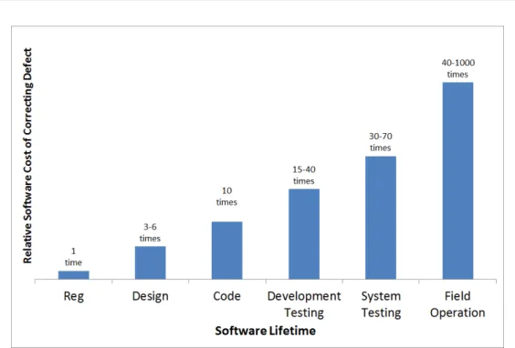
showed that the earlier a defect is fixed, the less cost involved in fixing said defect1. It is cheaper to repair a defect early, as there are extra costs involved during the different stages of development (e.g. if a defect is found after a product has been distributed to customers there are complaint resolution; product return; support and warranty costs involved) [Pressman 2001]. Figure 2.2 shows the relative cost of correcting an error in a software system [Pressman 2001] during the different stages of development. The bar chart shows that it can be up to 40-100 times more expensive to fix after the system has been released, compared to the requirements stage. Defect prediction is therefore important as it indicates potential areas that could contain defects, allowing time and resources to be assigned to these areas of a software system that have a greater propensity to defects [D’Ambros et al. 2010]. This could help save companies money as they are not fixing defects discovered later on in the development of a software system.

There are other costs involved with software defects which do not relate to financial costs. Defects can reduce the confidence a user has with a software system and/or what the system represents. For example, the user sign up problems during the initial phase of the ObamaCare website2registration, which opened in the USA in 2013. The ObamaCare website was meant to allow Americans in certain states to easily check if they are eligible for health subsidies after a new law was formed in the US called the “Affordable Heathcare Act”3. However, the website was poorly implemented and the site had many faults, which prevented citizens from signing up to or logging into the website [Connor 2013]. This affected the trust people had in ObamaCare, which was meant to be easy to sign up to. The website’s failures were used to attack the new US heath care act the website was meant to help implement [Dann 2013]. As the website’s problems were used to damage the act, Obama’s political relations were damaged too, with Obama commenting “And let’s admit it, with the website not working as well as it needs to work, that makes a lot of supporters nervous” [Connor 2013]. The cost of fixing the faulty website was reported to be $121m [FoxNews 2014]. The use of defect prediction could have allowed the developers to find defects before the system was released to the public, which could have saved ObamaCare from public ridicule and the extra cost of fixing the faulty website.

1_{The same could be said of a illness in a human. Machiavelli said that in the beginning of the malady it is easy to cure}

but difficult to detect, but in the course of time, not having been either detected or treated in the beginning, it becomes easy to

detect but difficult to cure. [Machiavelli 1997]

2_{www.healthcare.gov}

3_{The A}_ff_{ordable Care Act was implemented to put US citizens in charge of their health care. It is meant to give the}

(27)

2.1. Software Defect Prediction 11

Figure 2.2: A bar chart showing the costs of defects within a software system at different stages of development. The costs rise due to the extra costs of fixing a defect at different stages of the development. Shown inPressman[2001].

2.1.1 Performing Software Defect Prediction

Software defect prediction using machine learning is an automated method of determining potentially defective areas in a particular piece of software code. The predictions could make it possible for the developer to focus on areas of the software system before release, reducing the time and effort of find-ing defects by other means. Software defect prediction relies on three main components; dependent variables, independent variables and a model. Dependent variables are the defect data for the particular module or code. The defect data can be binary, or it can be continuous. Section2.1.2discusses depen-dent variables and how they are extracted in more detail. Independepen-dent variables are the metrics which can describe the software code, how it has changed or who changed it. Independent variables come in two forms, software code metrics; those that can be derived from the software code itself, and process metrics; metrics that measure the change of software code or software practices over time. Independent variables are discussed in more detail in Section2.1.3. The model contains the rule(s) or algorithm(s) that predict the dependent variable from the independent variables. These rules can be as simple as the number of independent variables in the model, or be as complicated as decision trees4 and regression5 techniques. Figure2.3shows a diagrammatic representation of how defect prediction is carried out. Test and training data is made up of either dependent or independent variables. The training data is used to create a classifier. A classifier is an algorithm that is used to create the model that will be used to predict potential faults. This model is then tested by predicting where potential faults are in a system using the independent variables. To determine if these predictions are correct, the dependent variables from the test data are used. This will determine the performance of the model, by being able to calculate certain performance measures. There are many machine learning models currently being used to predict the

4_{A decision tree algorithm is one that creates a graph of decisions based on the chance of an event happening.}

(28)

Figure 2.3: A diagram showing how defect prediction can be carried out.

location of defects in software systems. A study byHall et al.[2012] has identified over 200 papers and the models/metrics used to carry out defect prediction.

2.1.2 Dependent Variables (Defective or Not?)

Dependent variables in defect prediction are the variables that indicate if a module is defective or not. The dependent variables in defect prediction can be categorical (i.e. a module is defective or not) or continuous (i.e. the number of faults in a module). A defect can come in two forms - a pre release or a post release defect. A pre release defect is one that is found by programmers during the development or by testers in the testing phase of development [IEEE 2010]. A post release defect is also known as a fault. A post release defect will only manifest itself as a fault when a user experiences a failure with the product [IEEE 2010]. This means that a defect could lie dormant within a software product. Section 2.1.2.1below gives an example of the life cycle of both types of defect.

2.1.2.1 A Defect’s ‘Life’

A defect normally follows the same life cycle [IEEE 2010]. This life cycle can be used to determine the defectiveness of a module. An example of the ‘lives’ of two defects, one pre release and one post

(29)

Defect inserted March 2013

Failure Occurs Defect report created

December 2013

Defect fixed March 2014

Defective code

Figure 2.4: A Defects’s ‘Life’- this timeline shows the life of a defect within a software system. The defect was introduced in March 2013 and is not fixed until a year later. During this time, the code that is affected by this defect is labeled as defective (the red line).

release, is described below.

Thierry is a software developer at Zero Programming. In March 2013, he is tasked with developing a new feature for their popular tax reporting software. Unfortunately, Thierry unintentionally programs two defects (defect A and B) into one of the methods that he created. Defect A is found during the testing phase of development and is fixed by Thierry and is therefore recorded as a pre release defect. However, during the testing phase Defect B passes the current tests and is compiled into the final product. Defect B lies dormant for around nine months. In December 2013, a user experiences a failure from the software due to Defect B and files a defect report. This defect report is added to Zero Programming’s defect report database and means that Defect B has become a post release defect or a fault. Another developer, Patrick, is assigned the task of fixing the fault. A full year later after Defect B was introduced, the fault is fixed by Patrick and he files the defect report as fixed.

Figure 2.4 shows the timeline of Defect B which was present in Zero Programming’s tax software system. The use of this timeline allows the identification of methods which are defective at any stage of the products development. If the insertion and fix point dates are known then at any point in between these two dates (the red line on Figure2.4), the method will have been defective. If one knew the method introduced by Thierry in the example above is defective in November 2013 then the defect insertion and fix dates are known. The insertion and fix points of a defect are found in this dissertation by using the algorithm described by ´Sliwerski et al.[2005]. This algorithm is described in more detail in Chapter4. Dependent variables can be predicted by a model to forecast if a module is defective or not. This result can then be tested to see if the forecast is correct or not. This testing can help determine the recall and precision of the model. Precision and recall are measures of relevance of the data used. Precision is a measure of the accuracy of the model used to predict defects (i.e of all the instances predicted defective, how many are actually defective). Recall is the measure of relevant retrieval of instances (i.e. how many instances are identified by the model as defective out of all those defective instances that should have been returned).

Precision is calculated as follows (whereD=number of defects): precision= |Drelevant∩Df ound|

|Df ound|

(2.1)

and recall is calculated as:

recall= |Drelevant∩Df ound| |Drelevant|

(30)

2.1.3 Traditional Independent Variables (Software Metrics)

There are many different traditional independent variables that are used within defect prediction [Hall et al. 2012]. Sections2.1.3.1and2.1.3.2detail these independent variables, describing which have been used, why they were used and how effective they have been.

2.1.3.1 Source Code Metrics

Previous work on features of code in relation to defects has focused on defining and evaluating source code metrics (SCM). SCM measure particular code features (e.g. lines of code, object oriented metrics and complexity metrics). These metrics and the studies they appear in are described below.

Lines of Code LOC was introduced as a simple measure that allows the use of size to indicate potential defective areas of a software system. Some of the advantages of using LOC is that LOC are very quick to calculate and easily transferred across programming languages. One of the first defect prediction models proposed byAkiyama[1971] was based on lines of code (LOC).Akiyama[1971] proposed a regression model for determining the number of defects in the code based on the LOC. LOC measure the lines of code in a particular module, file or package. Studies differ in their interpretations of a LOC, some studies will use code comments, some blank lines and others will omit these lines. Others use logical lines of code, which is where only the semi colons have been counted [Rosenberg 1997]. However,Rosenberg [1997] highlighted that the format of the LOC was irrelevant as they all correlate with one another. Fenton and Ohlsson [2000] analysed pre and post release defects of a large communications system. They found that LOC was good at ranking the most fault-prone modules. The results of theFenton and Ohlsson[2000] study have been replicated and confirmed by Andersson and Runeson[2007] and Galinac Grbac et al.[2013].Zhang[2009] confirmedFenton and Ohlsson[2000]’s results that there is a relationship between the LOC and defects at both package and file level.Ostrand et al.[2005] produced a simple LOC based model to predict defects in a large industrial system. They concluded that their LOC model was a good way of predicting defects, with the model finding around 70% of faults. Bell et al. [2006] used theOstrand et al.[2005] model on a different software system, an automated voice response system. In this studyBell et al.[2006] found that the LOC model was not as effective, only finding 55% of the defects. Gyimothy et al.[2005] found that LOC was a very significant indicator of defects by performing regression and machine learning analysis on the web program Mozilla6. Subramanyam and Krishnan[2003] produced the same result when they analysed a commercial Java/C++system.

LOC predicts defects with an average recall of around 70% and an average precision of 67%, across 17 studies [Hall et al. 2012]. A problem with LOC is that it measures only one coarse grained feature of code and may only provide limited insight into potential sources of defects. Measuring just the size of a module does not take into account the finer detail involved, for example how complex the code is or how the code interacts with the system. Collinearity between the size of the module and the defect density exists in LOC [Rosenberg 1997]. This makes some findings using LOC confirm a statistical property, rather than actually show a relationship between the size of a module and the defectiveness chance of that module.

(31)

a

b

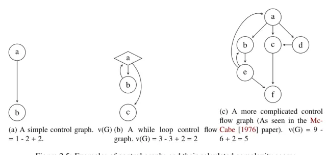
(a) A simple control graph. v(G)

=1 - 2+2.

a

b

c

(b) A while loop control flow graph. v(G)=3 - 3+2=2 a c b d e f

(c) A more complicated control flow graph (As seen in the Mc-Cabe [1976] paper). v(G)= 9 -6+2=5

Figure 2.5: Examples of control graphs and their calculated complexity scores

Complexity Measures Complexity measures were introduced to provide a measure of how hard soft-ware code may be to comprehend, test and maintain. The measures were formed in order to gain measur-able properties of the software and the relationships between these properties [Halstead 1977]. Halstead metrics [Halstead 1977] and McCabe’s complexity measure [McCabe 1976] were two of the first com-plexity measures introduced.

Cyclomatic complexity (CC) is based on the number of decisions in a program withMcCabe [1976] andHalstead[1977] having their own measures. CC measures the human comprehension of the code by identifying branching structures in code and calculating the number of logical paths through the code. The higher the CC number, the more complex the code and therefore the higher the probability of a defect being present.

To calculate the CC value you have to create a control flow graph of a particular module. A control flow graph is a representation of all paths of a module that could be traversed through a program during its execution. Figure2.5shows some examples of control flow graphs. Certain components of the control flow graphs are used to calculate CC. The number of nodes in a system (N). The number of times control is passed from one node to another, an edge(E). Finally, the exit node or the number of disconnected parts of the flow graph (P). Equation2.3 shows how these components are used to calculate the CC (v(G)) of any control flow graph (G).

v(G)=E−N+2P (2.3)

Halstead[1977] created a set of metrics that aimed to provide insight into code complexity and developer effort. The metrics are based on four base measures:

1. Number of unique operators7-n₁ 2. Number of unique operands8-n2 3. Total number of operators -N1

7_{Operators include assignments, blocks, labels, if statements, while statements and statement terminations (i.e. in Java}_;_).

(32)

Metric Equation Description Length N =N1+N2 Sum of all operators and all operands. A size metric

that is an alternative to LOC. Vocabulary n=n1+n2 Sum of all unique operators and operands. High values indicate harder to read code and therefore difficult to maintain. Volume V =N.log2(n) Another size metric. Describes the content in bits.

Difficulty D= n1

2 × N2

n2 Measures how difficult the code is to write, thus how error prone it may be. Level L= _D1 A low level score indicates less error prone code. Effort E =D×V Measures the effort to understand the code. The higher the metric the more difficult the code is to maintain.

Content C=L×V Language independent complexity measure

Error Estimate B= ₃₀₀V This metric aims to predict the number of validation bugs. 300 is the proportion of defects within the system. Programming Time (secs) T = ₁₈E How long it would take to program a particular module. 18 is a constant that reflects the number of decisions a programmer will have to make per second. Table 2.1: Halstead complexity metrics created byHalstead[1977].

4. Total number of operands -N2

These four measures form the basis of the algorithms shown in Table2.1. The CC measures have been heavily scrutinised due to the fact they assume certain constants (error estimate and programming time) and may only be a proxy for LOC [Fenton and Pfleeger 1998,Hamer and Frewin 1982,Shen et al. 1983, Shepperd and Ince 1994]. CC metrics again also only provide a subset of potential features that may be associated with the faultiness of potential code.

Ohlsson and Alberg [1996] carried out an investigation using a telecommunications system with the aim to study the relationship between defects and several graph metrics, including but not limited to, the number of branching points, number of branches and the number of possible paths. Ohlsson and Alberg [1996] also calculated McCabe’s complexity and wanted to predict which modules could be faulty before coding had already begun. Ohlsson and Alberg[1996]’s results showed that the metrics could predict the most fault prone modules before coding had started. Turhan et al. [2009] used CC alongside many other metrics to create a defect prediction approach for companies that did not track local bug data. Menzies et al.[2007] compared the use of metrics and models within defect prediction. Using the McCabe metric data taken from the NASA datasetsMenzies et al.[2007] were able to show that the SCM selected is not as important as which learning algorithm is used.

Object Oriented Metrics Following the introduction of new object oriented programming languages, researchers began to take advantage of the new metrics they could derive from the interactions between

(33)

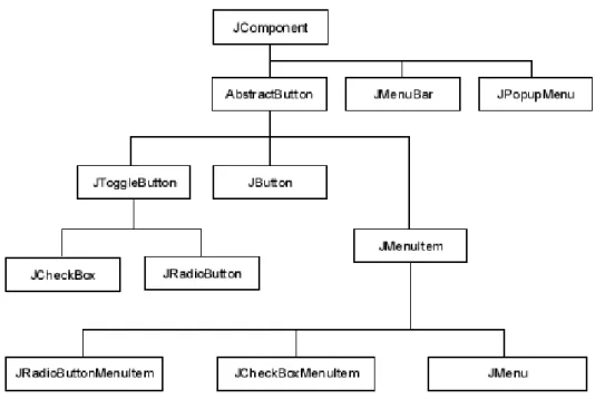
Figure 2.6: Inheritance between Swing classes in Java.

and within objects. Chidamber and Kemerer[1994] (CK) developed six Object Oriented (OO) metrics to measure the object oriented features of code. These six OO metrics focused on the complexity of classes within a system and how complexity can impact on maintenance and development. The metrics are based on the notion that the higher the complexity of a method and/or its class, the higher the potential for errors.

The CK metrics use the notion of inheritance within the code and mention trees, parents and children. These terms will be explained briefly. Inheritance is where a subclass (child) Yinherits all of the at-tributes and operations associated with its superclass (parent) X [Pressman 2001]. Inheritance is an important part of object oriented programming as it allows code reuse. An inheritance tree is similar to a family tree in that it is the full structure of how all the parents and children of a system are linked. Figure2.6shows an example of an inheritance tree. Each of the white rectangle boxes are an object in Java swing package. Each branch that flows down from an object is that objects children. The children inherit methods and attributes from its parent object. For example, aJMenuwill inherit methods from its parentJMenuItem. This is just a portion of the swing inheritance tree andJComponentwill have a parent andJMenucould have children.

The six OO metrics described are outlined below [Chidamber and Kemerer 1994]:

1. Weighted Methods per Class (WMC)- WMC is the sum of the complexities for all the methods in a class. The number of methods and the complexity of these methods is a predictor of the amount of maintenance needed for the class. The more methods in the class, the greater the impact on the children as the children inherit all the methods in that class. Classes with many methods are more likely to be application specific, limiting their reuse potential.

2. Depth of Inheritance Tree (DIT)- The DIT metric is the maximum length from the node to the root of the tree. DIT measures the amount of ancestor classes that can affect the class analysed.

(34)

Metric Description

FanIn Number of other classes that reference the class FanOut Number of other classes references by the class NOA Number of attributes

NOPA Number of public attributes NOPRA Number of private attributes NOAI Number of attributes inherited NOM Number of methods

NOPM Number of public methods NOPRM Number of private methods NOMI Number of methods inherited

Table 2.2: Class level OO metrics described in the defect prediction literature [D’Ambros et al. 2010]

The deeper the inheritance tree, the greater the number of methods that have been inherited. This makes it more difficult to predict behaviour. Deep trees mean there is a higher design complexity. 3. Number of Children (NOC) - NOC is the number of immediate subclasses subordinated to a class in the class hierarchy. It measures how many subclasses are to inherit the methods of the parent class. The greater the number of children, the greater the reuse, the greater the likelihood of improper abstraction of the parent class. If a large number of children exist, this could be a case of misuse of subclassing.

4. Coupling Between Object classes (CBO)- CBO is how many classes a single class uses. One class is coupled to another if it acts on the other. Generally the greater the coupling, the more detrimental to design as it prevents reuse. If there is low coupling, the class can be reused else-where. If there is a large amount of couples, then maintenance becomes bigger as the changes done in one class will effect other parts of the system.

5. Response For a Class (RFC)- This measures the amount of methods that can be executed in response to a message received by an object in that class. It also measures the potential com-munication between the class and other classes. The greater the amount of methods that can be invoked in response to an object, the greater amount of understanding required from the tester or developer. This means that the testing and debugging of the class is more complicated.

6. Lack of Cohesion in Methods (LCOM)- LCOM measures the count of the number of method pairs whose similarity is zero minus the count of method pairs whose similarity is not zero within a class. The larger the amount of similar methods, the more cohesive the class. Cohesiveness of methods in a class is desirable as it promotes encapsulation. A lack of cohesion implies that the class should be split into two or more subclasses. Low cohesion also increases complexity, thereby increasing the likelihood of errors.

Table 2.2 shows the other OO metrics that have been identified in the defect prediction literature [D’Ambros et al. 2010].

Basili et al.[1996] investigated OO metrics to see how effective they were as predictors. They inves-tigated eight medium sized information management systems written in C++. Basili et al. [1996]’s conclusions were that five out of the six CK metrics were useful predictors during the early phase of

(35)

development. The only predictor that was not good was the WMC metric [Basili et al. 1996]. Similar types of analysis have been performed byBriand et al. [1999], Chidamber et al. [1998],Janes et al. [2006],Li and Henry [1993],Ronchetti et al.[2006]. Each of the studies is performed on industrial C++projects, except forLi and Henry[1993] which was done in Ada. Each of the studies conclude that at least one or more of the metrics is good at predicting defects.El Emam et al.[2001] used metrics fromMcCabe[1976] and the metrics from theBriand et al.[1999] study to investigate different defect prediction models. El Emam et al.[2001] results showed that their model had high accuracy and that coupling had the strongest association with fault proneness. Briand et al.[1999] gathered their metrics from a commercial Java application. Briand et al.[1999]’s work showed that the coupling metrics had the strongest association with fault proneness.

Hall et al.[2012] show that in defect prediction OO metrics have a similar recall and precision as LOC, in 42 studies the average recall is around 65% and precision around 67%. Compared to LOC, the OO metrics do measure some finer grained features of code and also identify more of those features. However, these OO metrics are still only a small subset of possible code features.

Combination of Metrics Some studies have used a combination of SCM to generate their models. Arisholm and Briand[2006] used 32 different SCM in their defect prediction model. These metrics included those measuring the coupling between classes, the changes to code (e.g. fault corrections) and code quality (code style, practices and the amount of redundant code). They used the model on a large Java telecommunications system which has over 110K SLOC. Arisholm and Briand [2006]’s results showed that their model could reduce verification effort costs9 by up to 29%. Khoshgoftaar and Seliya [2004] used metrics based on “call graphs, control flows and statement metrics”. In total 28 metrics were used to compare seven different classification models, examples of these metrics included: procedure calls (call graphs), number of entry nodes (control flows) and LOC (statement metrics). Khoshgoftaar and Seliya[2004]’s results showed that software quality estimation models can improve the reliability of a software system, due to the models being able to target specific potentially defective areas of the code base.

2.1.3.2 Process Metrics

A process metric reflects the changes of a system over time [Henderson-Sellers and Henderson-Sellers 1996] (e.g. the number of code changes in a module). Process metrics are based on revisions and historic changes to files. They can take into account the amount of times the file or module has been changed due to defective code.

The histories of the revision control systems have been used to indicate defects in software systems. Table 2.3 shows an example of the process metrics introduced by Moser et al. [2008] based on the historical data from the revision control system.Moser et al.[2008] investigated whether change metrics are better predictors of defects than code metrics. They also wanted to analyse the cost associated with getting a prediction incorrect. They compared 31 code metrics to 18 change metrics over three different releases of Eclipse (2.0, 2.1 and 3.0).Moser et al.[2008] concluded that change metrics are a better predictor of defective code than code metrics. They also showed that files with a high number of revisions and files with bug fixing activities are the best indicators of potential defects. Whilst, heavily edited files or files included in a large CVS commit are less likely to be defective.

(36)

Metric Name Definition

REVISIONS Number of revisions of a file

REFACTORINGS Number of times a file has been refactored BUGFIXES Number of times a file was involved in bug-fixing

AUTHORS Number of distinct authors that have committed the file into the reposi-tory

LOC_ADDED Sum over all revisions of the lines of code added to a file MAX_LOC_ADDED Maximum number of lines of code added for all revisions AVG_LOC_ADDED Average number of lines of code added for all revisions LOC_DELETED Sum over all revisions of the lines of code deleted from a file MAX_LOC_DELETED Maximum number of lines of code deleted for all revisions AVG_LOC_DELETED Average number of lines of code deleted for all revisions

CODECHURN Sum of (added lines of code - deleted lines of code) over all revisions MAX_CODECHURN Maximum CODECHURN for all revisions

AVG_CODECHURN Average CODECHURN for all revisions

MAX_CHANGESET Maximum number of files committed together to the repository AVG_CHANGESET Average number of files committed together to the repository

AGE Age of the file in weeks

WEIGHTED_AGE Sum of (the Age of revision times the LOC added) divided by the sum of the LOC added

Table 2.3: List of Change metrics used in theMoser et al.[2008] study.

Graves et al.[2000] examined a telephone switching system which consisted of over 1.5 million LOC. Graves et al. [2000] approach was based on seven new measures derived from the revision history -Number of past faults, -Number of deltas (i.e. the amount of previous changes), the average age of the code, the development organisation, number of developers, how modules are connected (i.e. how many modules are changed together) and a weighted time damp model. The weighted time damp model computes a module’s fault potential by adding contributions from each change. A contribution is the level of fault potential, a large fault potential is c