Computational Astronomy: Classification of Celestial Spectra Using Machine Learning Techniques

SJSU ScholarWorks

SJSU ScholarWorks

Master's Projects Master's Theses and Graduate Research

Spring 5-20-2020

Computational Astronomy: Classification of Celestial Spectra

Computational Astronomy: Classification of Celestial Spectra

Using Machine Learning Techniques

Using Machine Learning Techniques

Gayatri Milind Hungund

Follow this and additional works at: https://scholarworks.sjsu.edu/etd_projects

Part of the Artificial Intelligence and Robotics Commons, External Galaxies Commons, and the Other Astrophysics and Astronomy Commons

A Project Report

Presented to

Dr. Robert Chun

Department of Computer Science

San José State University

In Partial Fulfillment

Of the Requirements for the

Class CS 298

By

Gayatri Milind Hungund

May 2020

ii © 2020

Gayatri Milind Hungund ALL RIGHTS RESERVED

iii

Computational Astronomy: Classification of Celestial Spectra Using Machine Learning Techniques

By

Gayatri Milind Hungund

APPROVED FOR THE DEPARTMENT OF COMPUTER SCIENCE SAN JOSÉ STATE UNIVERSITY

May 2020

Dr. Robert Chun Department of Computer Science Dr. Thomas Austin Department of Computer Science

i

Computational Astronomy: Classification of Celestial Spectra Using Machine Learning Techniques

by Gayatri Milind Hungund

Lightyears beyond the Planet Earth there exist plenty of unknown and unexplored stars and Galaxies that need to be studied in order to support the Big Bang Theory and also make important astronomical discoveries in quest of knowing the unknown. Sophisticated devices and high-power computational resources are now deployed to make a positive effort towards data gathering and analysis. These devices produce massive amount of data from the astronomical surveys and the data is usually in terabytes or petabytes. It is exhaustive to process this data and determine the findings in short period of time. Many details can be missed out and can lead to increased errors. Machine Learning can thus be applied for automated intelligent data analysis and recognition in the field of astronomy to gather important information and recognize or classify star types. Celestial Spectral Classification is one such problem that needs to be addressed using Machine Learning and will help astronomers to know whether the classified star has particular physical or chemical properties. Machine Learning can help astronomers to determine the class of celestial spectra which in turn can help in determining various properties of the star and will make the classification process

intelligent, automated and less cumbersome.

Keywords: Machine Learning, Astronomy, Stellar Spectra, Classification, Multi-layer Perceptrons, K-fold Cross-Validation, Sampling, Hidden Layers, Neural Network

ii

I would like to take this opportunity to thank my Master’s project advisor Dr. Robert Chun for helping and motivating me to move forward with a different and challenging topic, research in depth about the solutions implemented and also helping me find resources related to the project. I would also like to thank Dr. Aaron Romanowsky for helping me getting started with my project and pointing me towards excellent resources related to astronomy and Machine Learning, and Dr. Thomas Austin for timely support and technical help during the entire course of project for in-depth research on the research topic. I also take this opportunity to thank Dr. Martin Luther King Jr. Library for providing me with excellent online resources and research articles for this research. I also thank my family for their constant motivation throughout the project timeline.

iii

Guoshoujing Telescope (the Large Sky Area Multi-Object Fiber Spectroscopic Telescope LAMOST) is a National Major Scientific Project built by the Chinese Academy of Sciences. Funding for the project has been provided by the National Development and Reform Commission. LAMOST is operated and managed by the National Astronomical Observatories, Chinese Academy of Sciences.

iv 1. Introduction ... 1 2. Research Objective ... 2 3. Introduction to Astronomy ... 3 3.1 Electromagnetic spectrum ... 3 3.2 Types of Spectra ... 4

3.3 Introduction to Stellar Spectra ... 6

3.4 Computational Terminologies ... 7

3.5 Stellar Spectra ... 8

4. Stellar Spectra Classification ... 9

4.1 Classification Types ... 9

4.2 Doppler effect in light waves ... 10

4.3 Factors affecting classification ... 13

4.3.1 Temperature ... 13

4.3.2 Metallicity ... 14

4.3.3 Surface Gravity and Radial Velocity ... 15

5. Technical Approaches ... 16

5.1 A survey of classification techniques ... 16

5.2 Classification using Neural Networks ... 17

5.3 Classification using random forest ... 18

5.4 Classification using clustering ... 20

5.5 Classification using Random Forest and Support Vector Machine (SVM) ... 22

6. Proposed System ... 25

6.1 System Architecture ... 25

6.2 Tools and Technologies ... 26

6.3 LAMOST Dataset ... 27

6.4 Dataset Features ... 28

6.5 Data Preprocessing and visualization ... 28

6.6 Outlier Detection ... 29

6.7 Feature Co-relation ... 33

6.8 Data Scaling ... 35

6.9 Synthetic Minority Oversampling Technique (SMOTE) and Splitting ... 37

v

7.1 Stochastic Gradient Descent (SGD) Classifier ... 45

7.2 Logistic Regression ... 48

7.3 Ridge Classifier Cross-Validation (CV) ... 51

7.4 MLP Classifier ... 52

8. Advantages Over Existing Approaches ... 56

9. Conclusion ... 57

10. Future Scope ... 58

vi

1. Wavelength Vs Intensity curve for understanding spectral properties ... 4

2. Working of Spectroscope ... 5

3. VTFS 102 ... 6

4. Sigma Orionis ... 6

5. Spectra types ... 8

6. H-R diagram ... 10

7. Red and Blue Shift ... 11

8. Pictorial Representation of shifts ... 12

9. Population II stars in M80 ... 14

10. Population I star in Rigel ... 14

11. Difference between the original and normalized spectra ... 17

12. Classification accuracy and Signal to Noise Ratio ... 21

13. Example of wavelength correction using shifting ... 23

14. System architecture and workflow ... 26

15. Distribution of available spectra in selected dataset ... 27

16. Data pre-processing and DataFrame Construction ... 29

17. DataFrame construction after feature selection and outlier removal ... 30

18. Demonstration of presence of outliers in selected dataset ... 30

19. Removal of outliers after application of Inter Quartile Range ... 31

20. Tableau dashboard of stellar feature data before outlier removal ... 32

21. Tableau dashboard of stellar feature data after outlier removal ... 33

22. Pearson Correlation Matrix for stellar spectra feature data ... 34

23. DataFrame before scaling using Robust Scaler ... 36

24. DataFrame after scaling using Robust Scaler ... 36

25. Summarization of sclaing process ... 37

26. Imabalance in the DataFrame before sampling ... 37

27. DataFrame after SMOTE sampling ... 38

28. Process of data splitting and SMOTE sampling ... 39

29. MLP Neural Network ... 40

30. Data Flow inside the Orion web-application ... 42

31. Orion dashboard home page ... 43

vii

35. Performance fluctuations with increase in number of iterations for SGD algorithm ... 48 36. Performance gain with increase in number of iterations for Logistic Regression ... 50 37. Performance gain with increase in number of splits MLP classifier ... 53 38. Performance gain with increase in number of hidden layes and neurons for MLP classifier .... 55

viii

Table 1. Temperature ranges for spectral types ... 13

Table 2. Tool Stack ... 26

Table 3. Performance as a function of log functions for SGD classifier ... 46

Table 4. Performance as a function of maximum number of iterations for SGD classifier ... 47

Table 5.Performance as a function of solvers for Logistic Regression ... 49

Table 6.Performance as a function of maximum number of iterations for Logistic Regression ... 50

Table 7. Performance as a function of regularization strength for Ridge classifier ... 51

Table 8. Performance as a function of number of splits for MLP classifier ... 53

1 CHAPTER 1

Introduction

Modern-day astronomers face a lot of difficulties in processing petabytes of astronomical data and performing statistical analysis based on the gathered data to infer the essential

characteristics about the stars. These characteristics include its surface temperature, the kind of gases that exist on the star, and the proximity of the star to supernova in its lifecycle. Spectral lines are the light rays emitted by a star that can help the astronomers to find this information. The study of spectra helped Edwin Hubble to determine the truthfulness of the big bang theory and the continuously expanding universe. The production of a large amount of data by Hubble telescope created hurdles for astronomers for pattern recognition within the acquired data.

Classification of stellar spectra combined with Machine Learning techniques simplifies the process of classification by automating it. This process of automation of statistical analysis is

applied to the results obtained from the Large sky Area Multi-Object Fiber Spectroscopic Telescope (LAMOST) survey after Gigabytes of pictorial, and numerical data was generated at the end of the study. Manual classification deals with analyzing spectral images individually by studying various characteristics to assign respective classes to the stellar spectra. The application of Machine Learning techniques helps in the automated classification of stellar spectra and speeds up the process of making critical astronomical discoveries.

Other significant astronomical surveys, such as the Bayron Oscillation Spectroscopic Survey (BOSS), and Sloan Digital Sky Survey (SDSS) have generated a large amount of data that can be treated as input for classification. These surveys provided important information about dark matter and Redshifts for 1.5 million Galaxies. These measurements and computations describe the baseline for the concluding structure of the universe and determine important characteristics specific to a particular class of stars.

2 CHAPTER 2 Research Objective

The objective of this research is the classification of the stellar spectra using the data obtained from LAMOST survey into four prominent classes namely A, K, G, and F. The classifier is implemented by using Multi-Layer Perceptrons (MLP) classifier, data pre-processing techniques, dimensionality reduction, and feature selection. Making optimal use of the Machine Learning modules helps in designing a smart solution for the classification of a massive amount of astronomical data without human interaction and speeding up this process by manifold.

The classification of stellar spectra is one of the most critical areas of research that needs Machine Learning implementation for smart classification. This classified data forms the

foundation for the astronomers to understand the physical & chemical properties of the star. The application of Machine Learning in the astronomical domain will help simplify computational astronomy and speed up the cumbersome classification process. Data pre-processing is a crucial step in the process of building a Machine Learning module in order to remove outliers and null values paired with data normalization. The presence of outliers disturbs the data distribution and forces the mean to be inclined towards the outliers.

Dimensionality reduction also helps in simplifying the problem by reducing the

dimensionality of the dataset for reducing the complexity of training, and proper feature selection is also performed before applying a Machine Learning algorithm to increase the accuracy of existing methodologies for classification of stellar spectra. Consequently, this research aims to find the answers to the problem of classification of the spectral data obtained from one of the well-known spectroscopic surveys based on data pre-processing, visualization, dimensionality reduction, and neural network.

3 CHAPTER 3

Introduction to Astronomy 3.1 Electromagnetic spectrum

Different types of rays together compose an electromagnetic spectrum ranging in a variety of characteristics. The frequencies are comprised of visible and invisible forms of waves that travel long distances. Altogether, the spectrum contains Infrared, Visible, Microwaves, Gamma,

Ultraviolet, X-rays, and Radio Waves. The electromagnetic waves have the lowest frequency, while the Gamma rays have the highest frequency. The visible spectra are encountered in everyday

activities such as switching-on streetlights. Distant stars emit Radio Waves, Microwaves, and Infrared Rays, and are used to understand broad range features such as the shape of the Galaxy, presence of dust, and chemical elements that constituting the star [1].

Frequency, wavelength, and energy are the standard units used to measure and study the radiation emitted from the stars. The wavelength measures the distance between the start and end of a wave in one cycle. When the wavelength is short, the frequency is high as more waves will pass in a given period of time, resulting in production of high energy. The waves start to dissipate while entering into the Earth’s atmosphere. There is a requirement of satellites to get data or capture these waves that are unable to reach the ground. The astrophysicists can gather meaningful data and make amazing discoveries from this data.

The light incident on the prism splits into seven different colors. This prism experiment that splits the white light into seven colors can be said to work as an elemental spectrometer. Chemical elements present naturally emit different kinds of spectra at different surface temperatures. The spectra obtained from a particular star helps in determining the chemical behavior of a star.

4

as Giants, Super Giants, and other types of stars. This helps in grouping similar type of stars together and can further help the astronomers in determining the phase of entire life cycle of a star. 3.2 Types of Spectra

Spectroscopy helps in getting a shared understanding of changes incurred in a particular celestial body, and the nature of electromagnetic radiation. Moreover, it also helps in finding the chemical composition, density, and surface temperature of the given celestial body. Robert Bunsen and Gustav Kirchhoff concluded that a compressed gas produces a continuous spectrum and depicts bright lines on a relatively darker background when expanded. Based on this phenomenon, a total of three types of stellar spectrum exist:

1. Complete spectrum – This type of spectrum contains all the seven colors seen in a Rainbow.

2. Bright-line spectra - These types of spectra are known as emission spectra, which is a property exhibited by Nebula or gases.

3. Dark line spectra - These types of spectra are emitted by stars or other celestial objects and known as absorption spectra.

Planck's curve is a wavelength vs. intensity curve that is plotted as shown below. From the curve it is inferred that every celestial object emits some amount of energy at all wavelength ranges from 0 to 19907 [2]. The relatively warmer star will emit more energy than the star having a cooler temperature, which will have more wavelength.

5

The wavelength of the light is the distance between the two successive peaks in a wave. The larger the distance, the lesser the frequency and amplitude of the waves. The intensity of the

radiation helps in finding the color of the star. For example, if the celestial object has a temperature of about 2000 Kelvin (K), then the star appears to be bluish-white. The star with temperature 2000 K (Sun) appears reddish orange. The equation E= hf calculates the energy of star where h is the Planck’s constant having value 6.32 x Js [2].

A spectrograph is a machine used to divide the light into different colors. Modern-day spectrographs use a technique known as a diffraction grating to split the light. When the beam of light passes through diffraction grating medium, it breaks into maximas that give out relatively more light than the minima. The angle between the two maximas is directly proportional to wavelength.

Spectroscopy is carried out at all the wavelengths and bands to check the celestial body for the physical and the chemical compositions.

The modern telescopes use the optical fibers for spectroscopy, which is also known as the multifiber spectroscopy. The spectroscopes generally have a prism-like mechanism that helps in splitting the white light into different colors when the light waves emitted by the stars enter the Earth’s atmosphere [3]. The following figure describes the high-level working of spectroscope:

6 3.3 Introduction to Stellar Spectra

Every celestial body emits light, and when the light emitted enters the Earth’s atmosphere, the spectra show absorption lines due to energy absorption. Every star has a different absorption spectrum due to the presence of various chemical elements as a part of the chemical composition of a star at varying temperatures. The spectral characteristic is the comparative study of the features of the electromagnetic spectrum, including wavelength, amplitude, and other different computational parameters.

These spectral characteristics are used to classify the spectra into one of the classes labeled as A, F, B, G, M, K, and O. Each alphabet indicates the characteristic temperature of the star, presence of particular chemical elements, and wavelength of the emitted light. The alphabets also indicate the possible color and luminosity class of the celestial object.

For example, a star having a temperature of approximately 40,000 K appears blue and is a type O star. The star VTFS 102 and Sigma Orionis are two examples of type O stars and are photographed in the following images:

Fig. 3: VTFS 102 [4] Fig. 4: Sigma Orionis [5]

7 3.4 Computational Terminologies

Flux is the measure of the number of light waves passing through a refraction grating per square unit of area. Based on the assumption, the light waves disperse in different directions when they travel away from the source. A diffraction grating, when placed near the source of light, produces higher flux than when placed away from the light source.

The amplitude of wave is the distance from X-axis to the peak of the wave on the Y-axis. Higher values of the amplitude indicate the high frequency and shorter wavelength. The wavelength is measured in Angstrom or Å. Amplitude is measured in Metre, and the frequency of the waves is measured in Hertz. This light energy emitted is measured in Electronvolt.

When white light is incident on the prism, it splits into seven different colors. This

phenomenon is known as the dispersion of light. Astronomers pass the light rays incoming from the distant stars through a spectroscope to analyze it and get a summary of the presence of chemical elements, the surface temperature, the orbital motion, and the age of the star.

Due to the property of producing low energy, radio waves are used to detect the motion of gas on the planet, while the infrared light is used to study the warm gases on it. X-rays are emitted by the matter surrounding the black hole, while gamma rays are produced from the free electron. All these properties together form a single wave, which helps in understanding more about a particular celestial body when analyzed for changes and spectral properties.

The study of these computational properties helps the astronomers to gain meaningful insights about the long distant celestial body. Splitting the light and studying the correlation between these computational parameters helps the astronomers to understand the mechanics of Galaxies far away from the planet Earth.

8 3.5 Stellar Spectra

A stellar spectrum typically consists of emission and absorption lines demonstrating several properties such as the velocity, magnetic field of the star, the winds on the star, and the velocity at which the matter moves on the star [6]. The following figure is a demonstration of three different types of spectra:

Fig. 5: Spectra types [6]

A continuous spectrum is similar to the spectrum observed when white light is incident on the prism. The light waves emitted by a celestial body with high surface temperature due to the presence of chemical elements in their gaseous state produce the emission lines [7]. When light rays pass through the atmosphere, there is absorption in energy, which results in the darkening of the color band, also known as the absorption lines [8]. These absorption lines differ with the presence of chemical elements and can help in determining the chemical composition of a star. This

9 CHAPTER 4

Stellar Spectra Classification 4.1 Classification Types

Stellar spectra can be classified in two different ways which are as follows: 1. Harvard classification

2. Morgan-Keenan (MK) classification

The Harvard classification labels the stars based on the surface temperature. The star is classified as one of the types, namely A, F, B, G, M, K, and O. The M and K classes can be further used to classify the star as bright Giant, Supergiant, Giant, Giant Dwarf, or a Sub-Dwarf [9]. Each class has ten subclasses labeled from 0-9, and every subclass has an associated luminosity type denoted by Roman numerals [9]. The Harvard classification based on the surface temperature categorizes the stars in such a way that the highest temperature objects are placed first, and the warmth of a star type goes on decreasing towards the end of the.

A Hertzsprung- Russel (H-R) diagram is used by the astronomers to know about the surface temperature of the star and various other physical properties of the star that change with

difference in temperature [9]. The horizontal axis denotes the temperature while the vertical axis demonstrates the corresponding luminosity.

Temperature and respective spectral class form the horizontal axis, while the luminosity and absolute magnitude together constitute the vertical axis. H-R diagram demonstrating the

10

Fig. 6: H-R diagram [9]

As observed in the above figure, the stars are categorized as Supergiants, Giants, Dwarfs, and Main-Sequence stars. High temperature and lower luminosity stars are White Dwarfs and classified into the classes B, A, and F. Stars with relatively high luminosity and less surface temperature fall into the category of Giants. Supergiants also fall under the category of A, G, F, and K. The

remaining stars in the Main-Sequence fall under all different categories, but some of them have a high temperature, which is more than 25,000 K. In contrast, the others show varying degrees of luminosity and temperature, making these stars turn blue to red [9]. The position of a star in this diagram helps to determine the state of the fusion of chemical elements.

4.2 Doppler effect in light waves

Considering an example of a person standing at a railway station, starting to hear the intensity of the sound of the horn of the train to be increasing as the train approaches the platform; when the same train starts moving away from the person, the sound fades away. This phenomenon is known as the Doppler Effect. Similarly, this effect is observed in the light waves.

As the light waves travel away from the source of the light, they appear to be less bright and will be more intense otherwise; as a result of this, the flux changes. It can thus be inferred that the

11

light waves have a longer wavelength as they travel away from the source of the light [10]. This phenomenon is known as the Redshift or Doppler Effect in the light waves. Redshift is observed when the light source moves away from the observer. Blueshift is seen when the light source moves towards the observer [10].

Redshift and Blueshift phenomena significantly affect the way a light wave or a spectrum can be represented and becomes one of the crucial characteristics to determine the spectral class. Redshift and blueshift are depicted in the figure below:

Fig. 7: Red and Blue shift [11]

As shown in the diagram above, the wavelength of light decreases as the host star moves closer to the Earth, which is called Redshift. When the light source moves away from Earth, the wavelength will get increased, causing Blueshift [11]. The Redshift cannot be seen easily in daily life since the speed of light source is sufficient to make an obvious observation. Hence, when a source of yellow light moves fast, it does not appear red due to insufficient speed [11]. When astronomers study planetary motions, they deal with very high orbital velocity, and due to this, the

12

spectra emitted by the object are checked for the presence of absorption lines shifted towards the red color. By measuring this shift in the bands, astronomers can measure the orbital velocity of the star.

The Redshift can be calculated by the following formula:

Z = (l"#$%&'%( – _l&%$+ l&%$+) [9]

The wavelength of star at rest is shown by the unshifted spectra and observed bands will tend to show some spectral shift towards the red color if there is presence of Redshift.

Following diagram clearly distinguishes the unshifted, Redshifted, and Blueshifted spectra from each other:

Fig 8: Pictorial representation of shifts [11]

As depicted in the image above, when the light rays pass through Hydrogen or when Hydrogen is heated so that it emits light energy, the atmospheric gas also absorbs some amount of energy resulting in the formation of dark bands. Hydrogen itself emits some amount of energy resulting in an emission spectrum at the same place of absorption spectrum observation.

One of the notable observations made was about the structure of the lines observed in the spectra. As per the mathematical computations, red light has the lowest frequency, while the blue light has the highest. The astronomers measure Blueshift in terms of how much does the light shift

13

towards blue color. The Redshift is measured by knowing the shift of light waves towards the red part of the spectrum [12].

As the universe is expanding continuously, most of the light emitted from the celestial bodies is Redshifted when it enters the Earth’s atmosphere. The objects that are far from the Earth appear to be Redshifted. For example, the spectra emitted by the Sun will be Redshifted as the Earth’s orbit is elliptical. Also, due to the proximity of some celestial stars from the Earth, they appear to be Blueshifted [12].

4.3 Factors affecting classification 4.3.1 Temperature

As per H-R classification, different stellar classes have varying ranges of temperature due to which a variety of temperature dependent parameters also become a part of this study of the

classification of the stellar spectra. Following are the temperature ranges for different four spectra classes:

Sr. No.

Class Temperature Range 1 A 7,500K – 11,000K 2 F 6,000K – 7,500K 3 G 5,000K – 6,000K 4 K 3,500K – 5,000K

Table 1: Temperature ranges for spectral types [17]

As discussed earlier, these temperature ranges also have an effect on other factors such as the metallicity and surface gravity. These features are co-related in such a way that they play an equally important role in determining the class of the star.

14 4.3.2 Metallicity

The matter formed after the Big Bang mainly consisted of Hydrogen and Helium. The milky way was divided into groups or classes of stars called the populations, which currently include three types arranged in increasing order of metallicity. Population III stars are hypothetical stars with no metals existing on the surface and are thought to be existing from the early time of universe

formation and are not observed directly [18]. The population II stars are metal-poor stars but contain a good number of Alpha elements and are generally found in the globular clusters. Population I stars are the new metal-rich stars and are found in spirals of the Galaxy [18]. One example of metal-rich star is the Sun in our solar system. Metal-poor stars have metallicity value less than -1 while metal rich stars have metallicity greater than -1. Following pictures demonstrate the examples of population I and population II stars:

Figure 9: Population II stars in M80 [19] Figure 10: Population I star in Rigel [18]

The metallicity of star plays a crucial factor in determining the chemical composition of a star. A star is known to be metal-rich if there is an abundance of other chemical elements than Helium and Hydrogen. The metallicity of stars affects the temperature and color of the star. The

15

metal-rich stars are redder, which correlates them to have a lower temperature than metal-poor stars, which are blue and have a high temperature. Since the temperature plays a significant part in stellar spectra classification, the metallicity of the star also needs to be taken into consideration for classification.

4.3.3 Surface Gravity and Radial Velocity

Another feature that is inversely proportional to temperature is the surface gravity; the higher the temperature, the greater is the effect on the value of gravitational force. This

phenomenon can be related to black holes considered to have a high gravitational pull and similarly can be proven with Curie-Weiss law, which states that the magnetism is inversely proportional to temperature [20].

The radial velocity related to the observed and calculated Redshift. It is defined as the change in displacement of the planetary body with respect to a fixed point. The radial velocity method is one of the spectroscopic methods to determine the Redshift.

16 CHAPTER 5 Technical Approaches 5.1 A survey of classification techniques

A. Luo et al. [13] in 2004 utilized the collection of the variety of stars, Galaxies, and

Quasars using the LAMOST dataset with data size of more than one terabyte. Popular surveys such as Roentgensatellit (ROSAT), Faint Images of the Radio Sky at Twenty-Centimeters (FIRST), and SDSS together form a dataset containing almost 10 million celestial bodies. The data mining is performed by limiting the query type to one of the two supported query types. The first query type supports data retrieval using endpoints of the sky defined by the user, and the second query type uses indexing a Structured Query Language (SQL) table to retrieve specific data. The data retrieved can be used either for clustering or classification.

Clustering identifies the pattern between the selected properties to find groups of data different from each other. A classic example of clustering would be identifying Narrow-Line Quasars (NLQ) from celestial objects using the K-means clustering algorithm. Classification

determines the behavior or class to which a particular type of data is said to be belonging to base on the existing data. Ongoing research classifies the Galaxy spectra using dimensionality reduction techniques such as Principle Component Analysis (PCA) and neural networks.

Zaritsky et al. [13] also tried to study the morphological and spectral classification methods to examine the relationship between both the computational quantities. Castalander et al. [13] have studied the Balmer breaks to classify the spectra into five different classes. Many researchers have studied and classified the distant stars and labeled them as per the spectral classification type. Various studies include the study of the emission and absorption spectra, which allows the scientists to label the star and classify it into a given category.

17 5.2 Classification using Neural Networks

The LAMOST survey completed in the year 2008 and a large amount of data was generated for data analysis and statistical pattern recognition. The low-resolution spectra were difficult to classify. L. Tu et al. [14] have proposed the use of neural networks for the classification of spectra. The proposed system was divided into two parts consisting of feature extraction, data

normalization, and classification of spectra and determination of luminosity classes. The luminosity classes range from I to V and help in determining the temperature of the star.

The solid celestial bodies radiating heat generate continuum spectra. The spectral type is determined using continuum spectra and normalized spectrum. The normalization is achieved by first extracting the high frequencies in the spectra and determining the low-frequency components using the wavelet method. The spectra are then reconstructed and fitted to produce normalized spectra. The figure below illustrates the original and normalized spectrum for A0V:

Fig. 11: Difference between the original and normalized spectra [14]

The classification technique used is based on the usage of back propagation neural network. A typical neural network depicts the simulation of a brain and is used in classification of stellar spectra. The Back Propagation (BP) concept in the neural networks is applied to minimize the error.

18

After the input provision, a weight is assigned to each neuron, and the output of each layer is calculated. After obtaining the final output, Backpropagation (BP) can be applied to travel back to hidden layers and assign corrected weights accordingly to reduce the error in the output. This process is repeated until the most correct value is obtained as output.

In the proposed system, the spectra of class A is labeled using the number 3, and successive types are one more than the previous one. The BP neural network used in the experiment was configured to be of the type 481-i-1 [14]. The chosen BP network has one hidden layer and uses the radbas function to ensure non-linearity. The radbas calculates the exponent of -n squared for a particular value of n. Here, n denotes the weighted sum of inputs and the weights assigned to the hidden layers [14].

The stellar spectra are labeled in such a way that O is labeled as 1, B is labeled with 2; hence the subtype O2 will be labeled as 2.2. The number of nodes in the hidden layers varies from 5 to 50, and 12 hidden layers yielded minimal test error. The data were selected from three different libraries, Silva, Jacoby, and Pickles, with a total of 359 spectra having a wavelength range from 3600 to 6000 Angstrom [14].

The training set consisted of 181 and 178 samples and earned a standard deviation of 0.2259 for spectral subtypes. A standard deviation of 0.1997 was observed for the main spectral types. The proposed methodology was, however, not used to test on a higher number of dataset samples, and feature extraction was also not used before or after pre-processing [14].

5.3 Classification using random forest

Z. Yi and J. Pan [15], in the year 2010, have used the Random Forest classification

algorithm for the classification of stellar spectra. Random forest is an ensemble learning technique used for classification [15]. A random forest consists of the forest of trees that made by using feature selection based on entropy and information gain concepts. Entropy measures the

19

randomness in the data, and information gain measures how much information is given by a feature. The feature with the highest information gain is selected as the root node for the new split. Each tree is constructed using the features selected based on information gain, and the result is obtained by aggregating the results of different trees.

Random forest algorithm uses the method of data sampling using the replacement to

generate bootstrap samples, which are smaller subsets of the training sets [15]. The smaller subsets are then treated as training datasets for the decision trees with greater depth, and are used to create a random forest all together [15]. The final classification output of the random forest is the majority of the results produced by the individual decision trees. While selecting a particular set of data as a training set, the tuples of data that are not selected are known called ‘out of the bag.’ About 37% of the data obtained in the experiment carried out by the authors is not selected in the construction of decision tree and is utilized to predict the accuracy of the algorithm and to predict the correct outcome on test dataset which is also known as Out Of the Bag (OOB) error.

The dataset used for the classification experiment contained 131 spectra ranging from 1159 to 25000 Å sampled at 5 Å interval. The classifier is developed using the R programming

and randomForest package [15]. The classification problem relating to stellar spectra is solved by gaining deeper insight into the effect of temperature on the stellar class of the star. Due to a direct relation between different classes of star and temperature of the star, this problem is treated as the regression problem [15]. The strength or the correctness of the trees is decided by the number of features or mtry, which is one-third of the total number of trees in the random forest and ranges between 10 to 1000 [15].

Another critical feature used was ntree, which decided the number of trees to be present in the random forest and is set to a value from range 20 to 1000 [15].

20

The nodesize will be set to a maximum depth of trees. The performance of the random forest is evaluated using the Mean Squared Error (MSE) of out of the bag samples, which are the

residuals. Rsq or pseudo-R-squared ranges from 0 to 100 %, which measures the wellness of the match of actual observation vs. the expected observations. It is calculated to measure performance. A high value of Rsq is an indicator of good performance of the algorithm.

The experiment was carried out by setting the value of mtry to one of the values from {10,50,150,300,400,500,600,800,1000}, nodesize to 5 and ntree to 1000. Average MSE is calculated by running the code thrice. Similarly, ntree was varied from

{20,50,100,300,600,800,1000} and mtry was kept to 400. It was concluded that MSE was lower for a higher number of trees and mtry. The most optimal possible combination of parameters was found to be mtry = 400 and ntree = 1000, which had an output of average MSE to be 1.957 and Rsq of 98.96%.

Very high accuracy is obtained for this method of classification used for studying the spectral data. Random forest classification used the best tree selected from the solution space of trees, which means that it selected the solution that had the highest information gain, and hence accuracy is more as compared to other classification techniques. Boosting can be applied in this case to evaluate if the accuracy still can be increased.

5.4 Classification using clustering

J. Bin et al. [16] in the year 2016 have proposed the classification of spectral data obtained from the SDSS by applying Principle Component Analysis (PCA) as a feature extraction technique and then using clustering technique for classification. The dataset selected was the subset of SDSS, which is the Bayron Oscillation Spectroscope Survey (BOSS). The signal to noise ratio is

considered to be one of the crucial components in deciding the accuracy of the proposed system. The following figure shows the effect of the signal to noise ratio on accuracy:

21

Fig. 12: Classification accuracy and Signal to Noise Ratio [16]

As shown in the figure, all types of stars show the accuracy of classification above 95% for the signal to noise ratio of about 60 to 70. The proposed approach drops out the spectra exhibiting the signal to noise ratio less than 10. Principle Component Analysis (PCA) is used to convert data into a linear form and used as a dimensionality reduction technique [16]. The technique selects the cluster centers and allows the point to be a part of a particular cluster if the distance of the point is less from a specific center of the cluster and relatively higher than other points.

The clustering technique used in the algorithm makes the use of local density, which is calculated by the summation of a function of actual Euclidean distance between two points from which the cut-off distance is subtracted. The calculation of cut-off distance is done mathematically in such a way that a maximum of 2 percent of the entire set of dataset samples will lie in each cluster.

Principle component analysis is used to calculate and highlight the most prominent spectral characteristics and is a part of pre-processing. This technique helped in determining distribution based on selected features, which was clearly observed after plotting two principle components. The clustering based on densities was applied for classification by calculating Euler distance

22

between selected two points and then calculating the distance matrix parallelly [16]. The local density is calculated as mentioned earlier and the distance between the points having high local density is calculated as well. The cluster centers are then decided on the basis of the minimum distance calculated.

After determining the cluster centers, the outliers are detected and removed. Also, after plotting the cluster centers interesting observation was made that consisted of recognition of cataclysmic variable stars. The execution time for principle component analysis for 1142 type A0 spectra takes around 5.82 seconds and is faster than local outlier factor method by approximately 1 second. Similarly, for all other types of spectra the principle component analysis outperforms the local outlier factor and shows the accuracy of the classification algorithm to reach to 90% for B6 and 88.43% for A0 type spectra [16].

5.5 Classification using Random Forest and Support Vector Machine (SVM)

M. Brice and R. Andonie [9] in the year 2019 have also proposed a method to deal with the classification of spectroscopic data, which avoids the use of complex pre-processing methods, and uses the Random Forest and Support Vector Machine (SVM) classification techniques for spectral classification. The feature selection method used was Fisher feature selection, and the best results were obtained using the Random Forest classifier [9]. The dataset used was SDSS dataset

containing wavelength and flux measurements. The dataset contained the wavelength and flux measurements and was used to pre-process and then find the classification results accordingly.

As mentioned in the earlier section, the Redshift is calculated by subtracting the wavelength of the planetary body at rest from the wavelength of light observed to be radiated from the star. This wavelength is divided by the wavelength of light emitted from the star at rest to get the resulting Redshift. Data pre-processing is one of the most important steps before applying the Machine Learning algorithm. Proper data pre-processing techniques, if not applied, can lead to wrong results

23

generation and limited accuracy. The dataset used in the implementation of the algorithm is obtained as a fraction from the SDSS dataset consisting of 6,00,967 spectra [9]. The dataset consisted of the spectra that could be classified as one of the O, B, A, F, G M, or K class.

As a part of data pre-processing, the flux intensity was adjusted to and scaled to values between 0 to1 using a min-max scaler. Due to different values of flux measured from different datasets, these measurements were averaged out for every 5000 spectra. Redshift related pre-processing was implemented by applying the correction, and by the construction of a template wavelength matrix. As showed on in the figure below, the wavelength is first compared with every other value in the template and then shifted to the right, creating a missing value on the first

position. The missing wavelength is then replaced with the average of last K flux measurements [9].

Fig. 13: Example of wavelength correction using shifting [9]

The feature selection algorithms applied were Fisher and Chi-Square algorithms, after which the Support Vector Machine (SVM) and Random Forest Classifier were used to classify the spectra. The experiments were conducted by first pre-processing the data and applying the Redshift corrections, as mentioned earlier. Then the feature selection techniques are used to calculate the feature rankings of 1,10,000 samples [9]. The data splitting technique used is 10-fold

cross-validation for each subset of data, and the accuracy of the algorithm is computed by calculating the F1 score, precision, and recall.

The 10-fold cross-validation is applied with Fisher selection and under-sampling on 12,584 samples of data using random forest and SVM classification algorithm to obtain an accuracy

24

percentage that ranges from 81.177% to 84.95% for Random Forest and 60.43% to 66.51% respectively. For the artificial rest spectra, the accuracy ranges from 83.46 % to 87.40% for Random Forest and 55.63% to 66.81% for SVM [9].

The 10-fold cross-validation is applied with Fisher selection and hybrid sampling on 3,67,004 samples of data using random forest and SVM classification algorithm. An accuracy percentage ranging from 94.65% to 96.87 for random forest algorithm and from 96.30% to 97.58% was obtained after experimentation [9]. Precision, recall, and F1 score was found to be highest for 500 samples, which was approximately 0.96 with the application of random forest, hybrid fisher selection for Redshifted spectra [9]. Similarly, the F1, precision, and recall scores for the artificial rest spectra were approximately 0.97. The accuracy of these techniques resulted in 4% more accuracy than using just SVM for classification.

25 CHAPTER 6 Proposed System 6.1 System Architecture

The high-level view of the proposed system comprises four main components. These three components work in harmony to form a stellar spectra classification system. These components of the proposed methodology are listed as follows:

1. Data Pre-processing. 2. Data visualization.

3. Machine Learning module. 4. Orion dashboard.

A sample of data from LAMOST data release 5 version 3 AFGK catalog data is

pre-processed to form a DataFrame. Data analysis techniques, such as feature selection and scaling aid in the efficient analysis of data and promote higher accuracy. To study the data for the presence of outliers, DataFrame is divided into class-specific DataFrames, which means that a separate

DataFrame for class A, another separate DataFrame for class K, and so on. Feature correlation is studied after the application of IQR. The updated DataFrame is then scaled and sampled before passing it on to the MLP classifier.

The MLP classifier predicts the classes for test data obtained by splitting the dataset using Stratified K-fold cross validation. The performance of the algorithm is then studied by calculating the precision, recall, and F1-score of the model. An essential part of the proposed system is the Orion dashboard that provides an interactive platform for astronomers for stellar spectra

classification. Astronomers enter the values for various features through the dashboard, and the stellar class prediction is then displayed back on the panel after the machine learning module recognizes the class for the given spectra data.

26

Following architecture diagram gives a bird’s eye view of different components integrated together to form the stellar spectra classification system:

Fig. 14: System architecture and workflow

The entire workflow, tool-stack, and experimentation for the proposed system is described in the following sections.

6.2 Tools and Technologies

A wide variety of tools and technologies were used in the implementation of proposed system. These tools, technologies and libraries can be mainly divided into 3 possible groups:

1. Data Exploration and Visualization 2. Machine Learning

3. Orion web tool design

Following table enlists these tools in a systematic manner:

Sr. No. Module Tools, Technologies and Libraries

1 Data Exploration and Visualization

Tableau, Matplotlib, Seaborn

2 Machine Learning SciKit Learn, Pandas, SciPy, Imblearn 3 Orion web application design Flask, HTML, CSS, Python, Google Fonts

27

The dataset consisted of 45 columns describing different types of information, including information about geospatial coordinates, surface gravity, temperature, radial velocity, and associated magnitude. This data undergoes preprocessing, data exploration, visualization, data training, normalization, after feature elimination, and then produces the result that classifies the spectra into their respective classes.

6.3 LAMOST Dataset

The dataset selected for the proposed implementation is randomly sampled from the latest catalog version of the 5th data release of the LAMOST survey. The LAMOST survey has identified 90,26,365 spectra from the year 2011 to 2017 [21]. The catalog data made available depicts the information about stars, Quasars, Galaxies, and other unknown celestial objects constituting a massive amount of data. The selected subset of the dataset is a catalog download for data release 5, version 3, from the LAMOST AFGK Star Catalog. A total of 5,51,901 spectra of types A, F, G, and K are selected and sampled as training and test datasets for the Machine Learning model. The data distribution of available spectra in the selected dataset is as depicted in Tableau graph below:

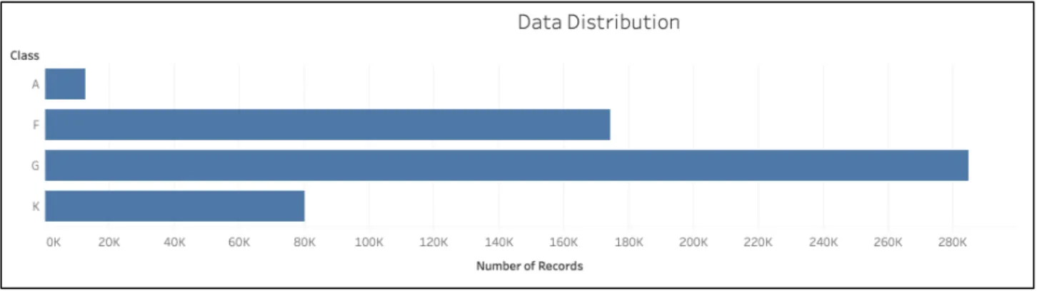
Fig. 15: Distribution of available spectra in selected dataset

The Tableau graph depicts that, the dataset contains 15,268 spectra of class A; 1,64,685 spectra belonging to class F; 2,54,679 spectra of class G; and 68,642 spectra of class K

respectively. The graph clearly demonstrates that the data is unbalanced which is a natural problem and is handled with proper scaling to reduce the training error

28 6.4 Dataset Features

The subset of data selected for the research contains 45 columns in total, and it was studied to understand the features that would be considered for an obvious choice of feature elimination. Higher dimensionality data is tricky to work with and can cause a higher rate of training errors. The dataset contained columns describing values for features including observation ID, stellar class, effective temperature, surface gravity, metallicity, Redshift, heliocentric radial velocity, their

associated errors, and signal to noise ratios of different filters [21].

To reduce the dimensionality of the dataset, the features including observation ID,

observation date, observation number, fiber ID, right ascension, declination (as they only give the location of the star), signal to noise ratios of filters, observation errors, object type, fiber type, comments, data source, input catalog and dates in Julian format were eliminated.

As these features are discrete numerical values and may not have as much effect on

determining the class of stellar spectra, these features were not taken into account for building the classification module. The correlation between heliocentric radial velocity, effective temperature, associated magnitude (ugriz magnitude), Redshift, metallicity, and surface gravity was studied. Relationship between these features was studied, and then the Machine Learning model was applied accordingly.

6.5 Data Preprocessing and visualization

The subset of data obtained from the LAMOST data release 5, version 3, contained records separated by a pipe or “|” and needed to be converted to Comma Separated Value (CSV) to produce a DataFrame for further data processing. The dataset was obtained by reading the file line by line, splitting it, and then creating a DataFrame; each line was later appended to the file as one record in DataFrame. The entire process of DataFrame construction consumed a total of 5 days due to the

29

abundance of data. The pre-processor is implemented in Python, keeping in mind the fastest working file handling techniques for big file sizes.

To generalize the stellar spectra classification, the subclass, for example, A0V, is considered to be ‘A’ due to limited computational resource availability. The suffixes appended to the class A determine the subclass and luminosity class of the star. The proposed system recognizes the stellar class of the star. In this example, it is denoted by ‘A’.

The dataset containing null values as a part of a record significantly affects the accuracy of the Machine Learning module and induces training errors. Missing data or null values can cause training errors; hence, as a part of data pre-processing, these values were searched and dropped out of the dataset to avoid training errors. The process of data pre-processing and DataFrame

construction can be summarized as follows:

Fig. 16: Data pre-processing and DataFrame Construction

6.6 Outlier Detection

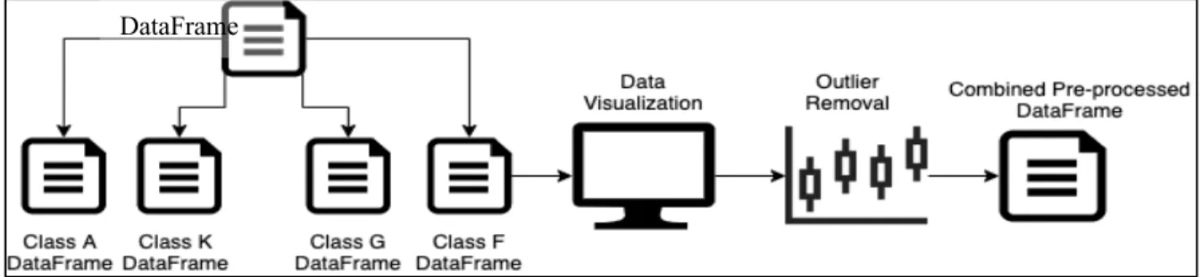
The preliminary step to building any machine learning module is effective analysis and visualization of data to understand the spread of data and pre-process it accordingly. To detect the presence of outliers, each class of spectra was split into a respective DataFrame, which lead to the formation of 4 DataFrame, one of each class. The process of splitting and application of IQR can be visualized as follows:

30

Fig. 17: DataFrame construction after feature selection and outlier removal

Before the outlier removal, the features including observation date, observation ID, and right ascension are removed, and only relevant features that have maximum impact on stellar spectra classification are selected. The purpose of splitting the DataFrame into class-specific data shards is to properties of each stellar class separately and apply IQR on DataFrames individually. After the outlier removal, the individual DataFrames are combined to produce pre-processed DataFrame containing the stellar spectra of all four classes.

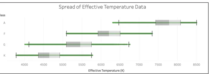
An interactive data visualization dashboard was implemented using Tableau, which showcased the spread of data and the presence of outliers. The visualization below shows the spread of the

temperature feature across all classes, clearly demonstrating the presence of outlier

Fig 18. Demonstration of presence of outliers in selected dataset

The above box plot clearly shows the presence of outliers, which can cause mispredictions and decrease training accuracy. In an effort of outlier detection and removal, the Inter-Quartile Range (IQR) is used to detect the outlier based on one of the conditions stated below:

31

1. Let Q1 be the lower quartile, Q3 be the higher quartile, and the IQR be denoted by Q3-Q1. Any of the data points lying outside these ranges are outliers and are eliminated. The interquartile ranges work in such a way that 1 percent of values before and after the start and the end of quartile are removed by inducing the range in which there are no outliers:

Lower limit = Q1 – 1.5*IQR [22] Higher limit = Q3 – 1.5*IQR [22]

2. As the dataset is split into 4 DataFrames, the outliers are removed from DataFrame belonging to each stellar class individually. IQR is then applied to each DataFrame to remove outliers. Then, these DataFrames are combined into one main DataFrame, and data is shuffled randomly to reduce the bias and can now be used for classification. The classes A, F, G, and K, are numbers 0, 1, 2, and 3 respectively for the ease of understanding. The following is an example of the

feature temperature from the dataset after removing the outliers in the data:

Fig 19. Removal of outliers after application of Inter Quartile Range

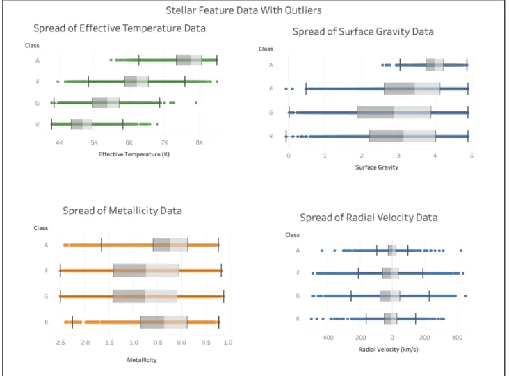
Other important features are studied for outliers, and an interactive dashboard is developed using Tableau as comparative study of data with outliers vs. data after outlier removal using IQR as a part of data visualization. The data was connected to Tableau software, and box plots were used to study the IQR ranges of data with respect to each class.

32

The Tableau dashboard below demonstrates a comparative study of subset features before outlier removal:

Fig. 20. Tableau dashboard of stellar feature data before outlier removal

As depicted in the above figure, the colored dots indicate the presence of outliers that need to be removed to increase the efficiency of the Machine Learning module. Hence, IQR was used for outlier removal and a Tableau dashboard was made to depict the data after outlier removal. IQR helped in removal of outliers and stabilized the data before applying the Machine Learning

algorithm. This process of outlier elimination also resulted in the generation of less false negatives or more false positives.

Following is the screenshot of Tableau dashboard demonstrating a comparative study of subset features after outlier removal:

33

Fig. 21. Tableau dashboard of stellar feature data after outlier removal

6.7 Feature Co-relation

Different features have varied effects on the data and need to be studied carefully to consider only the highly co-related features for analysis. As explained in the earlier section, the temperature has a direct effect on Redshift as the spectral bands get widened with an increase in temperature. On the other hand, the temperature is inversely proportional to metallicity. A similar trend is observed with surface gravity and radial velocity as well. All these features help in getting the highest co-relation in understanding the feature interdependency.

The selected features include the magnitudes of filters u, g, r, i, z, j, and h indicated by mag1, mag2, mag3, and so on. Filters, effective temperature teff, radial velocity denoted by rv, surface gravity logg, Redshift z, and metallicity denoted by feh. These features are studied to have

34

an impact on the classification of stellar spectra and hence selected to train the Machine Learning module.

Highly dimensional data increases the chances of higher inaccuracies and misclassification; hence, redundant features, including observation date, ID, comments, and the source, are eliminated in pre-processing. The DataFrame, including the selected features, is now studied for correlation between the features for better application of MLP classifier.

The correlation between the different features was studied well as the features with lower or no association were eliminated to increase the efficiency of the Machine Learning algorithm

applied to the dataset. With the purpose of understanding the feature correlation, the Pearson correlation matrix is constructed using the Seaborn package for the constructed DataFrame, which is displayed as follows:

Fig. 22. Pearson Correlation Matrix for stellar spectra feature data

The correlation matrix describes how closely the data features are related to each other. Positive correlations indicate an increase or decrease in values of both features with respect to each

35

other, indicating direct proportionality. In contrast, the negative ones indicate inverse proportionality [23]. The value 0 shows no correlation between the two features.

As per the Pearson correlation matrix constructed for the proposed system described in Fig. 19, the negative correlation value of -0.018 for temperature teff and metallicity feh indicates inverse proportionality; meaning, stars with higher temperatures tend to be metal-poor. The positive

correlation value of 0.11 indicates direct proportionality between surface gravity and metallicity. The associated magnitude and Redshift show a very low correlation of -0.00032. But, both of these features are strongly correlated with remaining features and hence cannot be removed.

The associated magnitudes of filters are wavelength-specific and used to predict the

Redshift, and since the wavelength is directly related to Redshift and thus cannot be removed from the DataFrame. The type ‘u’ filter shows the highest correlation value of 0.11 with Redshift. Due to the presence of some correlation between the features as indicated by the correlation matrix; hence all the features present in the matrix are given as inputs to the classifier.

6.8 Data Scaling

Due to the difference in units of measures for each feature, they have different ranges of values. For example, the temperature of a star can reside in the range of 5000 K to 10,000 K; on the other hand, the metallicity ranges from -1 to 1. The difference in measurement ranges can lead to low training speed and unequal contribution of the features toward the functionality. Thus, it necessary to scale the data to make all the features reflect a standard range of values to improve training speed and ensure an equal contribution. The following figure demonstrates the DataFrame before scaling:

36

Fig. 23: DataFrame before scaling using Robust Scaler

Fig. 20 demonstrates the snippet of data depicting the different ranges of measurement of features. As seen in fig. 20, Redshift values range from -0.000027 to -0.000158, temperature ranges from 4659.20 to 6711.95, and magnitudes range from 0 to 99. This scenario is a clear indicator of different scales and thus should be scaled using an appropriate scaler.

Scaling experimentation was conducted by making the use of different types of scalers such as a MinMax scaler, standard scaler, MaxAbsScaler, and robust scaler from the Scikit learn library. Robust scaler proved to be the most efficient for the given type of data and was used for scaling the pre-processed DataFrame as the accuracy score for the prediction made after scaling the data using Robust Scaler is 91% accurate.

The Robust Scaler proved to be more effective in increasing the accuracy of MLP classifier due to the use of IQR in data pre-processing. Robust scaler scales the data without considering the median for each feature individually, and the data is transformed into the required format [30]. The scaler was configured with centering set to true and scaled to IQR.

The following figure shows the snippet of data after normalization using Robust Scaler:

37

As depicted in Fig. 24, the data is now scaled to the same range for each feature, which helped in faster training of the MLP classifier. Without the use of scaling, the MLP classifier takes 70.96 seconds to classify a number of stellar spectra with an accuracy score of 79.59%. After the application of scaling, the execution time is increased to 117.34 seconds, with an increased

accuracy score of 91.26%. Fig. 24 is also an indication of missing column class, which is present in Fig. 23 is removed since it is the target variable and should not be scaled. The process of obtaining the scaled data can be described in the figure below:

Fig. 25: Summarization of Scaling Process

6.9 Synthetic Minority Oversampling Technique (SMOTE) and Splitting As observed in the Fig. 26 the dataset is highly imbalanced. In addition, the following snippet of code output clearly shows the imbalance in the data:

Fig. 26: Imbalance in the DataFrame before sampling

The impact of using the unscaled, outlier containing unbalance data decreased the accuracy of the Machine Learning algorithms to the range of 70 to 81%. The presence of an imbalance in the data led to reduced accuracy; it also makes the algorithm biased, leading to misclassification. Thus, re-sampling is a pre-requisite before splitting the data into training and test datasets. The data can be either under-sampled, which eliminates the samples of data from the class having maximum samples or oversampled, which deals with re-sampling the minority data.

38

Neural network is sensitive to scaling and re-sampling and produces better results on application re-sampling as per experimentation. SMOTE applies the technique of oversampling the minority data samples by creating synthetic samples based on the existing ones to reduce imbalance in classes [28]. In the course of experimentation, SMOTE was used to over sample the minority data after outlier removal and scaling. Following snapshot depicts the values in dataset after sampling:

Fig. 27: DataFrame after SMOTE sampling

As depicted in Fig. 27, the number of data samples in class A increased to 1,97,428 from 12,388. The experimentation was carried out to result in an increase in accuracy score after the application of SMOTE. The effect was studied before and after splitting and scaling. Better results in terms of precision were obtained after the application of SMOTE after scaling and splitting. The accuracy of the MLP classifier was increased by at least 1%.

After removal of class imbalance, the neural network performs more efficiently as compared to classification applied on unbalanced data directly. The output application of SMOTE results in the training set of 5,62,027 samples.

Before using the classification algorithm, the data is split into training and test dataset using Stratified K-fold cross-validation. K-fold cross-validation used for splitting data on each iteration of the MLP classification algorithm resulted in decreased accuracy as compared to using stratified K-fold cross-validation. Stratified K-K-fold cross-validation resulted in increased accuracy due to the generation of uniform distribution of class samples. The number of folds was set to 10 after

39

experimentation as it resulted in maximum precision with shuffling enabled. The process of resampling and splitting can be summarized using the following figure:

Fig. 28: Process of Data splitting and SMOTE Sampling 6.10 Multi-Layer Perceptrons (MLP) Classification

A perceptron is a component of a neural network that consists of input and weight assigned to it for the calculation of output. Each perceptron has multiple inputs and produces one output. This output is then passed to a hidden layer for additional computation. The product of the sum of all the weights and the input is known as a weighted sum. Multiple Perceptrons grouped together form a neural network, which can be used for nonlinear classification.

The input signal moves through the hidden layers and then ultimately produces the output in the output layer. The deep neural networks are either feed-forward or backward pass neural

networks. The backward pass neural networks use the backpropagation strategy to reduce the loss and reach a state where the error is minimum, also known as convergence.

40

Following diagram demonstrates the architecture of a typical MLP Neural Network with 3 hidden layers, input nodes, and output node:

Fig. 29: MLP Neural Network

The MLP neural network described above consists of 3 hidden layers, an input layer with four inputs and an output node. The MLP classifier build for the proposed system consists of 5 hidden layers with ten neurons each. The values of hidden layers and neurons are set after experimentation resulting in the highest accuracy score.

For classification of stellar spectra into A, K, G, and F classes, MLP classifier is configured from Scikit learn and used to train on the sample dataset and predict the values for the class. The classifier was configured by setting appropriate values for activation function, hidden layers, random state, and maximum iterations. The value of alpha is set to 0.0001, which is the default value, and nervous momentum is enabled.

The activation function selected was the Rectified Linear Unit or relu, and the seed for the random number generator was assigned as 21 after experimentation. The maximum number of iterations was initially set to 10 and increased or decreased for studying increase or reduced

41

accuracy. Since the neural networks are sensitive to normalization, the data is scaled to increase the efficiency of the neural network.

The dataset initially consisted of 45 columns describing different types of stellar features, including information about geospatial coordinates, surface gravity, temperature, radial velocity, and associated magnitude. This data undergoes preprocessing, data exploration, visualization, data training, normalization, and then produces the result that classifies the spectra into their respective classes.

6.11 Orion Dashboard

This research aims to further simplify the stellar class recognition by introducing an

interactive web user interface “Orion” for prediction of the stellar class by adapting a user-friendly methodology. The astronomers or space enthusiasts enter the values for features displayed on the dashboard and then obtain classification results in real-time which speeds up and automated the class recognition process by manifold.

The web application is developed in Flask and Python for Representational State Transfer (REST) Application Programming Interface (API) development in backend paired along with Hypertext Markup Language (HTML) and Cascading Style Sheets (CSS) for front-end. The background images were obtained from Pixabay, and the image was edited using Polarr tool. The following flow diagram explains the working of developed web-application:

42

Fig. 30. Data flow inside the Orion web-application

The values for the features are taken as input from the user, and data from the form is

collected and stored in the input file. The Machine Learning module is already trained and ready for prediction as a part of separate code. This module keeps an eye on the creation of the input feature file. The implementation is similar to a cron job in the Linux operating system. Once the input file is available for prediction, the values are read, and the MLP classifier predicts the class of stellar spectra.

Once the class is assigned to the spectra, the output of this classifier is stored in an output file. Likewise, the web application also keeps an eye for the creation of this output file. Once the file is created, the output of the classification is displayed on the webpage.