Marquette University
e-Publications@Marquette
Electrical and Computer Engineering Faculty Research and PublicationsElectrical and Computer Engineering, Department of
9-1-2017
Data Improving in Time Series Using ARX and
ANN Models
Hermine Nathalie Akouemo Kengmo Kenfack Marquette University
Richard J. Povinelli
Marquette University, [email protected]
Accepted version. IEEE Transactions on Power Systems, Vol. 32, No. 5 (September 2017): 3352-3359. DOI. © 2017 IEEE. Used with permission.
Marquette University
e-Publications@Marquette
Electrical and Computer Engineering Faculty Research and
Publications/College of Engineering
This paper is NOT THE PUBLISHED VERSION; but the author’s final, peer-reviewed manuscript. The published version may be accessed by following the link in the citation below.
IEEE Transactions on Power Systems, Vol. 32, No. 5 (September, 2017): 3352-3359. DOI. This article is © Institute of Electrical and Electronics Engineers (IEEE) and permission has been granted for this version to appear in e-Publications@Marquette. IEEE does not grant permission for this article to be further copied/distributed or hosted elsewhere without the express permission from IEEE.
Data Improving in Time Series Using ARX and ANN Models
Hermine N. Akouemo
Department of Electrical and Computer Engineering, Marquette University, Milwaukee
Richard J. Povinelli
Department of Electrical and Computer Engineering, Marquette University, Milwaukee
Abstract:
Anomalous data can negatively impact energy forecasting by causing model parameters to be incorrectly estimated. This paper presents two approaches for the detection and imputation of
anomalies in time series data. Autoregressive with exogenous inputs (ARX) and artificial neural network (ANN) models are used to extract the characteristics of time series. Anomalies are detected by
performing hypothesis testing on the extrema of the residuals, and the anomalous data points are imputed using the ARX and ANN models. Because the anomalies affect the model coefficients, the data cleaning process is performed iteratively. The models are re-learned on “cleaner” data after an anomaly is imputed. The anomalous data are reimputed to each iteration using the updated ARX and ANN models. The ARX and ANN data cleaning models are evaluated on natural gas time series data. This paper demonstrates that the proposed approaches are able to identify and impute anomalous data points. Forecasting models learned on the unclean data and the cleaned data are tested on an
uncleaned out-of-sample dataset. The forecasting model learned on the cleaned data outperforms the model learned on the unclean data with 1.67% improvement in the mean absolute percentage errors and a 32.8% improvement in the root mean squared error. Existing challenges include correctly identifying specific types of anomalies such as negative flows.
SECTION I.
Introduction
Data cleaning is the process that consists of detecting and imputing anomalous data [1]. In the
energy domain, training accurate forecasting models requires data that correctly captures the underlying system. However, energy signals often contain anomalies, which can be due to various causes such as human error (e.g., mistyping) or system error (e.g., erroneous
measurement). During model training, anomalous energy signals yield erroneous forecasting models. Applying an erroneous forecasting model on out-of-sample signals yields inaccurate forecasts. Thus, anomaly detection and imputation is an important forecasting problem. Since domain knowledge is critical to determine whether a data point is anomalous, we limit our analysis to the energy domain.
This paper presents two novel approaches that combine time series models with hypothesis testing to detect and impute anomalies in energy time series. The time series models are an autoregressive with exogenous inputs (ARX) model and an artificial neural network (ANN) model. The contributions of the proposed algorithms are their ability to extract time series features using an ARX or ANN model, to use the residuals from applying the model to identify anomalous data points, and then to impute replacement values for the identified anomalies. Our approaches are able distinguish between anomalies and data points in the tails of the residual distribution by taking into account the statistics of the residuals and the number of samples in the data set.
The remainder of the paper is divided into three sections. Section II discusses previous work on data cleaning. Section III provides an overview of ARX and ANN modeling, along with the novel algorithms that combine time series modeling, hypothesis testing, and anomaly
imputation. The concluding section presents the results and analysis.
SECTION II.
Previous Work
Training accurate models in the energy domain requires anomaly-free training signals, where anomalies refer to data points that are considerably dissimilar to the remaining points in the data set [2]. Choy defines two types of time series anomalies: additive anomalies that are
isolated events and innovative anomalies that are errors propagated through time in the system [3]. Typically, additive outliers need to be deleted or replaced because they induce
biased variances and estimates [4]. Innovative outliers do not require a correction of the
measurements because they are usually noise [5]. In this work, we focus on additive anomalies.
Probabilistic techniques have been used for outlier detection in combination with a rejection threshold, hence yielding many false positives for large data sets [6]– [8]. However, in real data
sets, the underlying distribution of the data is not known, and there is not an optimal rule for choosing or calculating a rejection threshold.
Numerous authors have studied the impact of anomalous data in the parameter estimation of autoregressive integrated moving average (ARIMA) models [9]– [12]. Tsay investigated the
variance changes and level shifts caused by additive and innovative anomalies [13].
Autoregressive moving average with exogenous inputs (ARMAX) models also have been studied for outlier detection [14]–[17]. In statistical approaches, anomalies are data points that
deviate considerably from their predicted values [18]. Anomalies are detected by analyzing the
residuals (difference between actual and estimated values) because they affect the structure, parameters, and variance of the models [11].
Work in estimating ARIMA parameters includes Amini et al.[19], and Boroojeni et al.[20]. Amini
et al. presented an approach to forecasting electrical vehicle charging using a decoupled ARIMA approach. The parameters of the ARIMA model are tuned to improve performance [19].
Boroojeni et al. presented a two-tier demand forecasting approach to forecasting energy use and production on the smart grid. The two-tiers are a maximum likelihood estimator for longer durations and an ARIMA model for short term forecasting [20]. They have also used a
multi-seasonal ARIMA model to forecast the PJM interconnection [21].
The disadvantage of autoregressive moving average (ARMA) models for outlier detection is that the exact order of the polynomial functions for real time series data is difficult to determine
[22], [23].
Hawkins et al. and Zhang et al. studied outlier detection using neural networks [24], [25]. Neural
networks select one model from a set of allowed models with the goal of minimizing a cost function. An outlier in this case is an observation that does not conform to the pattern of the selected model [26]. Chen et al. presented a method for optimizing the parameters of ANN
model by using sieves, which are lower order versions of the model, and uses this approach to estimate the model parameters of three different types of ANNs [27], [28]. Bakirtzis et al.
developed a short-term load forecasting system using ANN to forecast demand for the Greek Public Power Corporation [29]. Sarwat et al. have used a ANN to predict the rate of weather
caused electrical system interruptions [30]. The advantage of neural networks are that they can
differentiate between anomalies from different classes. Weekley et al. also applied clustering techniques to a reconstructed phase space to detect anomalies [16]. To make valid and efficient
inferences about the data, anomalous data needs to be imputed after their detection.
Two approaches to identifying and imputing anomalies in energy time series are examined in this paper: ARX and ANN data cleaning models. Because of the potential presence of
anomalies, the learned parameters of the models may be biased [9]–[12]. To identify the
anomalies in the residuals and to avoid false positives by taking into account the number of samples in the residual distribution. We assume the residuals are normal. While this
assumption is violated in practice, it is useful to develop the theoretical aspect of the
technique. Hypothesis testing identifies anomalies in the tails of the distribution. Anomalies in this case are data points considered inconsistent with the distribution of the residual data set. Data cleaning consists of detecting and imputing anomalous data. Therefore, the anomalies identified are imputed using calculated replacement values [31]– [33]. The replacement values
also are calculated using ARX or ANN models.
As the anomalies are imputed, the estimation of model parameters improves. Therefore, the data cleaning process is implemented iteratively. The next section of this paper provides an overview of ARX and ANN modeling and describes the ARX and ANN data cleaning
algorithms.
SECTION III.
Methods
This section presents the methods used for outlier detection and imputation: the ARX and ANN data cleaning algorithms. The residuals are extracted with ARX or ANN models and the
anomalies are found on the residuals using the hypothesis-driven outlier detection algorithm.
A. Hypothesis-Driven Outlier Detection Algorithm
Hypothesis testing is a statistical technique that draws conclusions about a sample point by testing whether it comes from the same distribution as the training data [8]. A hypothesis is a
statement about the values of the parameters of a probability distribution [34]. Here, the
hypothesis tests whether the extrema of the residuals are likely drawn from the probability distribution of the residuals. The null hypothesis (H0) is that the extremum of the residuals is not an outlier, while the alternative hypothesis (Halt) is that the extremum of the residuals is an outlier. The null hypothesis is rejected in favor of the alternative with a level of significance α, the probability of committing a type I error. A type I error occurs if the null hypothesis is rejected when true, and a type II error occurs if the null hypothesis is not rejected when it is false. In this paper, we set α=0.01 .
Let the experiment be 𝐸𝐸 = {Classifyinganextremum}. The outcomes of the experiment 𝐸𝐸 are “outlier” or “not outlier.” If the probability of “outlier” in the experiment 𝐸𝐸 is p, the probability of “not outlier” is 1- p. Let the number of samples in the data set be 𝑛𝑛. Each classification of an extremum is an independent experiment. Therefore, the experiment 𝐸𝐸 is a Bernoulli trial. The problem is to find the number of Bernoulli trials needed to observe an “outlier” in at least 𝑛𝑛 trials and supported by the set of 𝑛𝑛 samples. This corresponds to the cumulative distribution function of a geometric distribution [35]. The number of Bernoulli trials should be less than the
level of significance α for the data point to be considered an outlier. By taking into account the number of samples and the probability of the data points, the hypothesis-driven outlier
detection algorithm sets an effective bound on how many potential anomalies there might be in a data set. Our hypothesis-driven outlier detection algorithm is presented in Algorithm 1.
Algorithm 1: Hypothesis-Outlier-Detection.
Require: X,α , assumed distribution Dist(𝑋𝑋,𝛽𝛽) % Choose the minimum 𝑥𝑥 and the maximum 𝑥𝑥 % values of X as potential anomalies
% Find the parameters of their corresponding distributions 𝑋𝑋𝑚𝑚𝑚𝑚𝑚𝑚← 𝑋𝑋 ∖ �𝑥𝑥�
𝑋𝑋𝑚𝑚𝑚𝑚𝑚𝑚 ← 𝑋𝑋 ∖{𝑥𝑥}
Distmin←estimate𝛽𝛽′𝑠𝑠𝑠𝑠𝑠𝑠𝑋𝑋min
Distmax←estimate𝛽𝛽′𝑠𝑠𝑠𝑠𝑠𝑠𝑋𝑋max
% Compute the probability that the potential anomalies % belong to the distribution of the remaining data points 𝑝𝑝𝑚𝑚𝑚𝑚𝑚𝑚← 𝑐𝑐𝑐𝑐𝑠𝑠(𝐷𝐷𝐷𝐷𝑠𝑠𝑡𝑡𝑚𝑚𝑚𝑚𝑚𝑚,𝑥𝑥)
𝑝𝑝𝑚𝑚𝑚𝑚𝑚𝑚 ←1− 𝑐𝑐𝑐𝑐𝑠𝑠(𝐷𝐷𝐷𝐷𝑠𝑠𝑡𝑡𝑚𝑚𝑚𝑚𝑚𝑚,𝑥𝑥) 𝑔𝑔𝑚𝑚𝑚𝑚𝑚𝑚 ←1−(1− 𝑝𝑝𝑚𝑚𝑚𝑚𝑚𝑚)𝑚𝑚 𝑔𝑔𝑚𝑚𝑚𝑚𝑚𝑚 ←1−(1− 𝑝𝑝𝑚𝑚𝑚𝑚𝑚𝑚)𝑚𝑚
% Determine if 𝑥𝑥 or 𝑥𝑥 are anomalous based on α
if(𝑔𝑔max <𝛼𝛼)∨(𝑔𝑔min <𝛼𝛼)then
% The extremum with the lowest p is the anomaly
if(𝑔𝑔min <𝑔𝑔max) then
outlierIndex←index(𝑥𝑥)
outlierIndex←index(𝑥𝑥)
end if else
% Exit condition: There is no anomaly in the data set.
outlierIndex←nil
end if
return outlierIndex
Algorithm 2: ARX-Data-Cleaning.
Require: time series 𝑦𝑦, exogenous inputs (𝑏𝑏,𝑛𝑛𝑚𝑚), ARmodel order 𝑝𝑝 potentialAnomalies ← true
Indices← ∅
while (potentialAnomalies) do
% Estimate ARX model and calculate the residuals
model←ARX(𝑦𝑦,𝑝𝑝,𝑏𝑏,𝑛𝑛𝑚𝑚)
residuals← Calculate-Residuals (model,𝑦𝑦,𝑏𝑏)
% Find the largest anomaly at the level of significance 𝛼𝛼 𝐷𝐷 ←← Hypothesis-Outlier-Detection (residuals,𝛼𝛼)
if𝐷𝐷== nilthen
% Exit condition: No more anomalies found
potentialAnomalies←false
else
% Calculate a naïve imputation value for the anomaly 𝑦𝑦[𝐷𝐷]←0.5(𝑦𝑦[𝐷𝐷 −1] +𝑦𝑦[𝐷𝐷+ 1]
%$ Re-estimate the ARX model
model←ARX(𝑦𝑦,𝑝𝑝,𝑏𝑏,𝑛𝑛𝑚𝑚)
% Impute all anomalies found and keep iterating
Indices←Indices∪{i}
forj = 1: Indices.length do
𝑦𝑦(Indices[𝑗𝑗])← Forecast (model,𝑦𝑦,𝑏𝑏, Indices[𝑗𝑗])
end for end if end while
return y, Indices
The advantage of our hypothesis-driven outlier detection algorithm is that it accounts for the number of samples when computing the likelihood that a data point is an outlier. Time series are not the outcomes of independent random processes. Therefore, the time series features are extracted with techniques such as ARX and ANN. The hypothesis-driven outlier detection considers the residuals of the ARX and ANN models as an ensemble of data points drawn from a distribution. The algorithm focuses on the anomalous data points. Most importantly, the algorithm detects points that are most unlikely to be drawn from the assumed underlying distribution, while avoiding false positive anomalies.
B. ARX Data Cleaning Algorithm
An ARX model is an autoregressive model with exogenous inputs. The ARX model assumes a stationary and invertible process [36]. The exogenous inputs come from an external system,
which in this work is based on energy forecasting domain knowledge. The autoregressive model can be viewed as the output of an all-pole infinite impulse response filter whose input is white noise. An ARX model is written as:
𝑦𝑦(𝑡𝑡) =𝑐𝑐+� 𝜙𝜙𝑚𝑚𝑦𝑦(𝑡𝑡 − 𝐷𝐷) 𝑝𝑝 𝑚𝑚=1 +� 𝜂𝜂𝑚𝑚𝑏𝑏(𝑡𝑡 − 𝐷𝐷) 𝑚𝑚𝑥𝑥 𝑚𝑚=0 , (1)
where 𝑐𝑐,𝜑𝜑𝑚𝑚, and 𝜂𝜂𝑚𝑚 are the constant term, the autoregressive coefficients, and the exogenous coefficients, respectively. The variables 𝑝𝑝 and 𝑛𝑛𝑚𝑚 are the orders of the autoregressive and exogenous inputs, respectively. The ARX model is written as ARX(𝑝𝑝,𝑛𝑛𝑚𝑚). An ARX(𝑝𝑝, 0) is
reduced to an autoregressive AR(𝑝𝑝) model. The ARX data cleaning algorithm is presented in Algorithm 2.
Algorithm 2 assumes that the order of the ARX model is known a priori. The residuals found after estimation of the ARX model form a distribution of points where anomalies are detected using hypothesis testing. After an anomaly is identified, the parameters of the ARX model are re-estimated with the anomaly replaced by a naive impute of
𝑦𝑦^(𝑡𝑡) =𝑦𝑦(𝑡𝑡 −1) +2𝑦𝑦(𝑡𝑡+ 1),
to ensure that the point is not a false positive and also to remove some contamination from the imputation model. The new signal is used in a forecasting model to calculate replacement values for all the anomalies. The estimate of the model parameters improves after each anomaly is imputed. The replacement values are substituted into the time series, and the process repeats until no more anomalies are identified.
C. ANN Data Cleaning Algorithm
An artificial neural network is used to learn time series features and predict future values. It is a suitable choice because of its capability to model nonlinear systems [37].
An ANN is an interconnected network of units (also called neurons), that operate in parallel and learn from examples (samples) [38]. The defining equation for an autoregressive ANN is
𝑦𝑦(𝑡𝑡) =𝑠𝑠(𝑦𝑦(𝑡𝑡 −1), . . . ,𝑦𝑦(𝑡𝑡 − 𝑐𝑐),𝑏𝑏(𝑡𝑡 −1), . . . ,𝑏𝑏(𝑡𝑡 − 𝑐𝑐)), (3)
where 𝑏𝑏(𝑡𝑡) and 𝑦𝑦(𝑡𝑡) represent the input and output of the models at time 𝑡𝑡, respectively. The lag of the system is 𝑐𝑐, and 𝑠𝑠 is a nonlinear function representing the ANN [39].
Algorithm 3: ANN-Data-Cleaning.
Require: time series 𝑦𝑦,𝛼𝛼, exogenous inputs 𝑏𝑏, delay 𝑐𝑐,Ratio Rtrain, Rvalidation, Rtest
potentialAnomalies←true Indices←∅
while (potentialAnomalies) do
% Fit data with a NARX network % Calculate the residuals
[residuals, estimatedFlow]← Calculate-Residuals (net,𝑦𝑦,𝑏𝑏)
% Find the largest anomaly at the level of significance 𝛼𝛼 𝐷𝐷 ←Hypothesis-Outlier-Detection (residuals,𝛼𝛼)
if𝐷𝐷== nilthen
% Exit condition: No more anomalies found
potentialAnomalies←false
else
% Use the values estimated by the neural network % to replace all anomalies found and keep iterating
Indices←Indices∪{i}
y[Indices]←estimatedFlow[Indices]
end if end while
return𝑦𝑦, Indices
The goal of the network is to learn associations (weights and bias values) between the set of input-output pairs. Because the neural network is small, the weights and bias values are updated using the Levenberg-Marquardt optimization because it is computationally efficient and converges quickly [40].
In this paper, 𝑦𝑦(𝑡𝑡) and 𝑏𝑏(𝑡𝑡) are the time series signal and the exogenous inputs, respectively. There is only one hidden layer, and there is a delay of one in the system. The neural network performs a one-step-ahead prediction to keep from learning the anomalies. The ANN is re-trained after an anomaly is imputed. The neural network architecture is presented in Fig. 1.
Fig. 1. Artificial neural network architecture.
Similarly to the ARX data cleaning algorithm, the ANN extracts time series features and
calculates the residuals. The anomalies are found in the residuals using the hypothesis-driven outlier detection algorithm. However, ANN models also use the same time series features to compute estimated values. Those estimates values are used for the imputation of anomalous data, so a naïve imputation is not necessary for the ANN data cleaning algorithm. The ANN data cleaning algorithm is presented in Algorithm 3.
The ARX and ANN data cleaning algorithms illustrate each step of the outlier detection and imputation processes. They also show the iterative nature of the data cleaning process. The next section of this paper presents the results.
SECTION IV.
Results
This section describes the data set used to test the data cleaning algorithms and presents the results obtained using the example data set.
A. Data
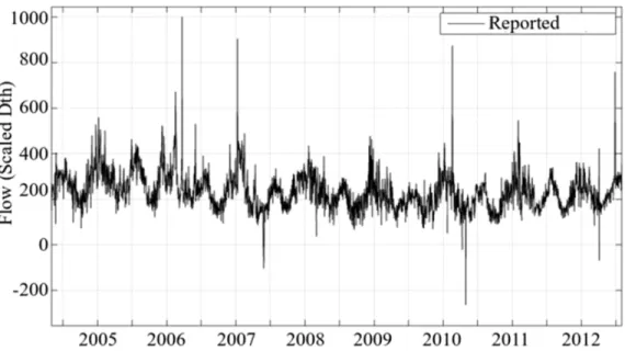
The data represents the daily consumption of natural gas recorded in the system of a utility in the United States. The data set ranges from 01 May 2004 to 31 July 2012 (𝑛𝑛= 3014). The data set is scaled to maintain confidentiality and is presented in Fig. 2.
Fig. 2. Daily natural gas reported consumption of a utility in the United States.
Because the time series data set is an energy-related signal, the exogenous inputs are weather-related. The exogenous inputs are the heating degree days wind-adjusted (HDDW) and the cooling degree days (CDD) [41].
If 𝑇𝑇 and𝑤𝑤 are the daily average temperature (°F) and wind speed (mph), respectively, the wind-adjusted HDD is
HDDW𝑇𝑇refH = max(72+𝑤𝑤80 ,152+𝑤𝑤160 )
× max(0,𝑇𝑇refH− 𝑇𝑇), (4)
where 𝑇𝑇refH is the heating reference temperature. Similarly, the CDD is defined as
CDD𝑇𝑇refC = max(0,𝑇𝑇 − 𝑇𝑇refC), (5)
where 𝑇𝑇refC is the cooling reference temperature. There is no influence of wind on warmer days. The base or reference temperature is the temperature below or above which heating or cooling is needed, respectively [42]. Multiple reference temperatures also can be used to
approximate the climate of a particular region.
For this example, the HDDW are calculated at reference temperatures 55 °F and 65 °F, and the CDD are calculated at reference temperatures 65 °F and 75 °F.
A delay of one is automatically incorporated in the system for the ANN data cleaning algorithm. In the case of the ARX data cleaning algorithm, one lag of HDDW and CDD are also used as exogenous inputs.
The data cleaning results are presented in the next sections.
B. ARX Data Cleaning Results
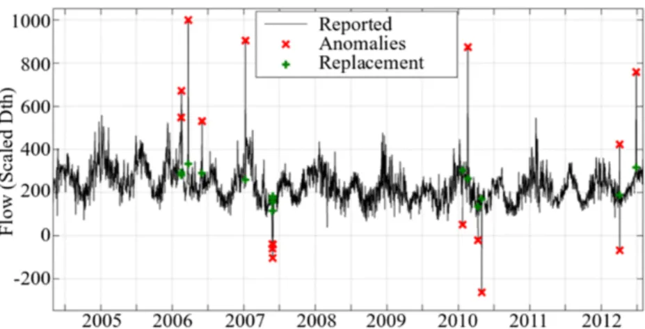
The results obtained using the ARX data cleaning algorithm are presented in Fig. 3 and Table I. The input in this case is the natural gas reported consumption, while the exogenous inputs are [HDDW55, HDDW65, ΔHDDW55, ΔHDDW65, CDD65, CDD75, ΔCDD65,
ΔCDD75]. The AR model order chosen is five. Fig. 3 and Table I depict the anomalies
Fig. 3. ARX data cleaning results on the natural gas data set using an AR model order of five.
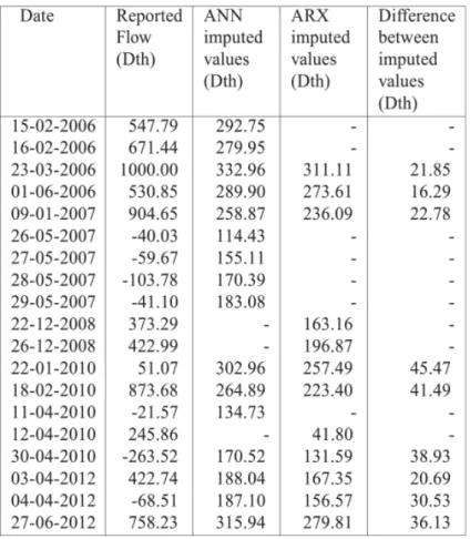
TABLE I Imputation Results for ARX Data Cleaning Algorithm
C. ANN Data Cleaning Results
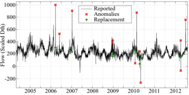
The outlier detection and imputation results for the ANN data cleaning algorithm are presented in Fig. 4 and Table II. The input in this case is also the natural gas reported consumption, while the exogenous inputs are [HDDW55, HDDW65, CDD65, CDD75]. The system has a delay of
one, which also introduces lag in weather signals. The ratio for randomly dividing the data set is selected to be 70% for training, 15% for validation, and 15% for testing. Fig. 4 and Table II present the anomalies found along with their original and imputed values.
Fig. 4. ANN data cleaning results on the natural gas data set.
A comparison between the ARX and ANN data cleaning results is discussed in the analysis section. The percentage of improvement that data cleaning provides to forecasting accuracy also is evaluated and presented.
D. Analysis
The imputation results for both the ARX and the ANN data cleaning algorithms are recapitulated in Table III. Table III shows that the ANN data cleaning algorithm found 16
anomalies versus 12 anomalies identified by the ARX data cleaning algorithm. Both algorithms identify different data points as anomalies, but they agree on nine data points being
anomalous. However, some obvious anomalies such as the negative flow values that occurred in May 2007 were not selected by the ARX data cleaning algorithm. Natural gas consumption can be zero but not negative. The AR model order selected is five, but the time series order is not exact. Therefore, we conclude that the ARX data cleaning algorithm can be improved using other techniques to find the AR order of a time series [43]. Also, the imputation results between
the ANN and the ARX are within a 5% margin (compared to the maximum value in the time series of 1000 Dth). We conclude that the results are consistent because both data cleaning algorithms use different forecasting models to calculate replacement values.
TABLE III Comparison of the Imputation Results for the ARX and ANN Data Cleaning Algorithms
To evaluate the improvement that data cleaning brought to forecasting accuracy,
out-of-sample errors are calculated for the original (unclean) data set and for both the ARX and ANN cleaned data sets.
The unclean and clean training sets from 01 May 2004 to 31 July 2011 are used to train the two forecasting models. Two error metrics are used. The first is the root mean squared error (RMSE) RMSE =�� (𝑦𝑦 ^ (𝑡𝑡)−𝑦𝑦(𝑡𝑡))2 𝑁𝑁 𝑡𝑡=1 𝑁𝑁 , (6)
where 𝑦𝑦(𝑡𝑡) is the actual flow at time 𝑡𝑡, 𝑦𝑦^(𝑡𝑡) is the estimated flow at time 𝑡𝑡, and 𝑁𝑁 is the number of observations. The second error metric is the mean absolute percentage errors (MAPE)
MAPE =100𝑁𝑁 � |𝑦𝑦^(𝑡𝑡)−𝑦𝑦(𝑡𝑡)𝑦𝑦(𝑡𝑡) |
𝑁𝑁 𝑡𝑡=1
, (7)
where 𝑦𝑦(𝑡𝑡) is the actual flow at time 𝑡𝑡, 𝑦𝑦^(𝑡𝑡) is the estimated flow at time 𝑡𝑡, and 𝑁𝑁 is the number of observations. The RMSE and MAPE are calculated on the test set from 01 August 2011 to 31 July 2012. It is important to note that the test set (out-of-sample) is not cleaned. In future work we will implement the two cross validation approaches of Hu et al. [44] The moving
approach fixes the length of the training and testing periods, but training starts at a moving time. The rolling approach lengthens the training set for each cross-validation.
The forecasting model is derived from Vitullo et al.[41].
𝑦𝑦^(𝑡𝑡) = 𝛽𝛽0+𝛽𝛽1HDDW55+𝛽𝛽2HDDW65+𝛽𝛽3∆HDDW55
+𝛽𝛽4∆HDDW65+𝛽𝛽5CDD65+𝛽𝛽6CDD75
+𝛽𝛽7sin(2𝜋𝜋DOW7 ) +𝛽𝛽8cos(2𝜋𝜋DOW7 ) +𝑠𝑠(𝑡𝑡).
The coefficients 𝛽𝛽𝑚𝑚,𝐷𝐷 = {1,2,3,4,5,6} are the coefficients of the weather-related inputs. The reference temperatures are 55 °F, 65 °F, and 75 °F. The weather variables used in this model are derived from forecasted temperature and wind speed. Multiple reference temperatures can be used to approximate the climate of a particular region. In that case, the forecasting model will have more coefficients. 𝛽𝛽0 is the non-varying amount of natural gas load related to
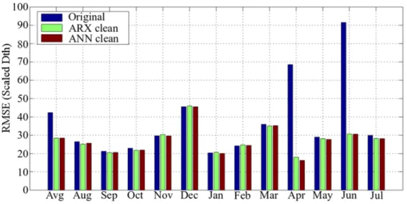
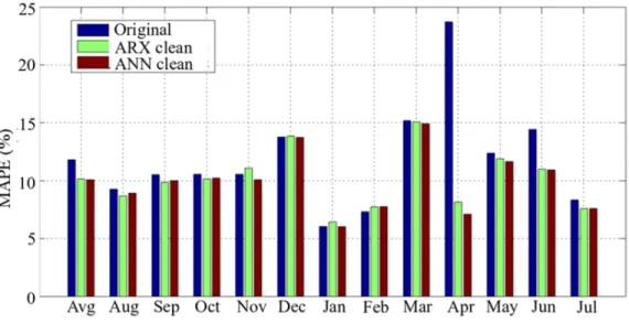
everyday uses such as cooking, water heating, and drying clothes. The coefficients 𝛽𝛽7 and 𝛽𝛽8 represent the variation of natural gas demand by day of the week (DOW). f(t) is used to model the effect of holidays and days around holidays on the natural gas demand. The out-of-sample forecasting errors are presented in Table IV, and Figs. 5 and 6.
TABLE IV RMSE and MAPE on Original and Clean Test Sets
Fig. 6. Comparison between MAPE on original and clean data sets from August 2011 to July 2012.
Table IV shows that all RMSE and MAPE calculated on clean data sets are smaller than RMSE and MAPE calculated on the original data set. Anomalies impact the estimation of the parameters of a time series data set, and imputing anomalies improves prediction models. For our test set, there is an average of 32.8% improvement in RMSE and a 1.67% improvement in MAPE. The maximum observed improvement is about 76% in RMSE and 16% in MAPE for April 2012. There is also an improvement of 66% in RMSE and 4.5% in MAPE for June 2012. Figs. 5 and 6 present a comparison between error measures calculated on the original data set and ARX and ANN cleaned data sets, and show that the largest improvements are observed in April and June 2012. They also show that the errors calculated using the ANN data cleaning algorithm results are smaller or about the same as the errors calculated using the ARX data cleaning algorithm results. The average difference between the ANN and ARX MAPE is 0.06%. The largest difference error of 1.06% in MAPE is obtained for April 2012 between the errors calculated using ARX and ANN cleaned data sets, confirming that the results are consistent because the differences of errors between the results from both data cleaning algorithms are small. Figs. 5 and 6 show also that the majority of the improvement in the overall error is due to the improvements in April and June 2012.
Both data cleaning algorithms yield good performance by comparing the percentage of
improvement obtained on forecasting accuracy. While the ARX data cleaning algorithm did not select some obvious outliers such as negative flow values, the error was considerably reduced by the data cleaning. The main advantage of the ANN data cleaning algorithm is that it does not require any additional forecasting model to calculate replacement values, and it does not require using other statistical techniques to calculate the AR order of the time series. The neural network model is robust because it is able to learn the structure of the time series features and uses the same features to calculate replacement values.
SECTION V.
Discussion and Conclusion
The proposed methods are applicable to a wide range of forecasting problems, given the proper domain knowledge. The domain knowledge is captured in the ARX and ANN imputation models. If our approach were applied to electric power data cleaning, an imputation model based on electric power domain knowledge would be used. We surmise that the imputation models for electric power would have similar inputs and structures, such as heating degree day and cooling degree day inputs as both natural gas and electric power consumption have temperature dependent characteristics.
The imputation models are intentionally simple in nature. The state-of-the-art forecasting methods are not appropriate for the proposed data cleaning approach. Sophisticated models are more likely to overfit the data and thereby learn the outliers, which would make the outlier identification more difficult. The use of a more sophisticated forecasting model is limited to the validation process, where we show that cleaned training data yields a better forecasting model. To the best of our knowledge the model we use for natural gas forecasting is state-of-the-art
[41].
Many techniques have been developed for data cleaning. This paper presents an approach for outlier detection and imputation based on autoregressive and artificial neural network models. The ARX data cleaning algorithm ensures that corrupted parameters are not used by doing a naive imputation before re-learning the model. The data cleaning results for the ARX and ANN data cleaning algorithms are consistent, but neural networks are robust enough to learn the characteristics of the time series and to provide residuals and replacement values. Therefore, an additional forecasting model for calculating replacement values is not necessary for the ANN data cleaning algorithm. The data cleaning algorithms are tested on the natural gas reported consumption of a utility in the United States and provide an average improvement of 32.8% in RMSE and 1.67% in MAPE on the test set.
The main contribution of this technique is the development of outlier detection algorithms based on hypothesis testing and using the number of samples in the data set and the
combination of time series modeling techniques to efficiently detect and impute anomalies in real time series data.
References
1 J. den Broeck, S. Argeseanu Cunningham, R. Eeckels, K. Herbst, "Data cleaning: Detecting diagnosing and editing data abnormalities", PLoS Med., vol. 10, no. 2, pp. 966-970, 2005.
2 D. M. Hawkins, Identification of Outliers, London, U.K.:Chapman and Hall, 1980.
3 K. Choy, "Outlier detection for stationary time series", J. Statist. Plan. Inference, vol. 99, no. 2, pp. 111-127, 2001.
4 C. R. Muirhead, "Distinguishing outlier types in time series", J. Roy. Statist. Soc. Ser. B, vol. 48, no. 1, pp. 39-47, 1986.
5 A. Kaya, "Statistical modelling for outlier factors", Ozean J. Appl. Sci., vol. 3, no. 1, pp. 185-194, 2010.
6 V. Barnett, T. Lewis, Outliers in Statistical Data, Hoboken, NJ, USA:Wiley, 1994.
7 G. Buzzi-Ferraris, F. Manenti, "Outlier detection in large data sets", Comput. Chem. Eng., vol. 35, no. 2, pp. 388-390, Sep. 2011.
8 M. Markou, S. Singh, "Novelty detection: A review—Part 1: Statistical approaches", Signal Process., vol. 83, no. 12, pp. 2481-2497, 2003.
9 I. Chang, G. C. Tiao, C. Chen, "Estimation of time series parameters in the presence of outliers", J. Technometrics, vol. 30, no. 2, pp. 193-204, 1988.
10 D. R. Martin, V. J. Yohai, "Influence functionals for time series", Ann. Statist., vol. 14, no. 3, pp. 781-855, 1986.
11 A. M. Bianco, M. Garcia Ben, E. J. Martinez, V. J. Yohai, "Outlier detection in regression models with ARIMA errors using robust estimates", J. Forecast., vol. 20, no. 8, pp. 565-579, 2001.
12 L. Denby, D. R. Martin, "Robust estimation of the first-order autoregressive parameter", J. Amer. Statist. Assoc., vol. 74, no. 365, pp. 140-146, 1979.
13 R. S. Tsay, "Outliers level shifts and variance changes in time series", J. Forecast., vol. 7, no. 1, pp. 1-20, 1988.
14 C. Fauconnier, G. Haesbroeck, "Outliers detection with the minimum covariance
determinant estimator in practice", J. Statist. Methodol., vol. 6, no. 4, pp. 363-379, 2009.
15 A. Grané, H. Veiga, "Wavelet-based detection of outliers in financial time series", Computat. Statist. Data Anal. Fifth Spec. Issue Comput. Econometrics, vol. 54, no. 11, pp. 2580-2593, Jan. 2010.
16 A. R. Weekley, R. K. Goodrich, L. B. Cornman, R. A. Weekley, R. K. Goodrich, L. B. Cornman, "An algorithm for classification and outlier detection of time-series data", J. Atmos. Ocean. Technol., vol. 27, no. 1, pp. 94-107, 2010.
17 A. Zaharim, R. Rajali, R. M. Atok, I. Mohamed, K. Jafar, "A simulation study of additive outlier in ARMA(11) model", Int. J. Math. Model. Methods Appl. Sci., vol. 3, 2009.
18 P. Tan, M. Steinbach, V. Kumar, Introduction to Data Mining, Boston, MA, USA:Addison-Wesley, pp. 651-683, 2006.
19 M. H. Amini, A. Kargarian, O. Karabasoglu, "ARIMA-based decoupled time series
forecasting of electric vehicle charging demand for stochastic power system operation",
20 K. G. Boroojeni, S. Mokhtari, M. H. Amini, S. S. Iyengar, "Optimal two-tier forecasting power generation model in smart grids", Int. J. Inf. Process., vol. 8, no. 4, pp. 79-88, 2015.
21 K. G. Boroojeni, M. H. Amini, S. Bahrami, S. S. Iyengar, A. I. Sarwat, O. Karabasoglu, "A novel multi-time-scale modeling for electric power demand forecasting: From short-term to medium-term horizon", Elect. Power Syst. Res., vol. 142, pp. 58-73, Sep. 2016.
22 G. E. P. Box, G. M. Jenkins, G. C. Reinsel, Time Series Analysis: Forecasting and Control, Hoboken, NJ, USA:Wiley, 2008.
23 G. E. Schwarz, "Estimating the dimension of a model", Ann. Stat., vol. 6, no. 2, pp. 461-464, 1978.
24 S. Hawkins, H. He, G. Williams, R. Baxter, "Outlier detection using replicator neural
networks", in Data Warehousing and Knowledge Discovery (Lecture Notes in Computer Science), vol. 2454, pp. 170-180, 2002.
25 Z. Zhang, J. Li, C. Manikopoulos, J. Jorgensen, J. Ucles, "HIDE: A hierarchical network intrusion detection system using statistical preprocessing and neural network
classification", Proc. IEEE Workshop Inf. Assur. Secur., pp. 85-90, 2001.
26 M. Markou, S. Singh, "Novelty detection: A review—Part 2: Neural networks based approaches", J. Signal Process., vol. 83, no. 12, pp. 2499-2521, 2003.
27 X. Chen, J. Racine, N. R. Swanson, "Semiparametric ARX neural-network models with an application to forecasting inflation", IEEE Trans. Neural Netw., vol. 12, no. 4, pp. 674-683, Jul. 2001.
28 X. Chen, "Large sample sieve estimation of semi-nonparametric models" in Handbook of Econometrics, New York, NY, USA:Elsevier, vol. 6, pp. 5549-5632, 2007.
29 A. G. Bakirtzis, V. Petrldis, S. J. Klartzls, M. C. Alexladls, "A neural network short term load forecasting model for the Greek power system", IEEE Trans. Power Syst., vol. 11, no. 2, pp. 858-863, May 1996.
30 A. I. Sarwat, M. Amini, A. Domijan, A. Damnjanovic, F. Kaleem, "Weather-based
interruption prediction in the smart grid utilizing chronological data", J. Mod. Power Syst. Clean Energy, vol. 4, pp. 308-315, 2016.
31 R. A. T. Donders, J. Geert, T. Stijnend, K. G. M. Moonsc, "Review: A gentle introduction to imputation of missing values", J. Clin. Epidemiol., vol. 59, pp. 1087-1091, 2006.
32 J. M. Jerez et al., "Missing data imputation using statistical and machine learning methods in a real breast cancer problem", J. Artif. Intell. Med., vol. 50, no. 2, pp. 105-115, 2010.
33 R. J. A. Little, D. B. Rubin, "The analysis of social science data with missing values", Sociol. Methods Res., vol. 18, no. 2/3, pp. 292-326, 1989.
34 D. C. Montgomery, Introduction to Statistical Quality Control, Hoboken, NJ, USA:Wiley, 2005.
35 A. Papoulis, U. S. Pillai, Probability Random Variables and Stochastic Processes, Boston, MA, USA:McGraw-Hill, 2002.
36 W. W. S. Wei, Time Series Analysis: Univariate and Multivariate Methods, Boston, MA,USA:Addison-Wesley, 2006.
37 H. T. Siegelmann, B. G. Horne, C. L. Giles, "Computational capabilities of recurrent NARX neural networks", IEEE Trans. Syst. Man Cybern. B: Cybern., vol. 27, no. 2, pp. 208-215, 1997.
38 D. F. Specht, "A general regression neural network", IEEE Trans. Neural Netw., vol. 2, no. 6, pp. 568-576, Nov. 1991.
39 S. Chen, S. Billings, P. Grant, "Non-linear system identification using neural networks", Int. J. Control, vol. 51, no. 6, pp. 1191-1214, 1990.
40 M. T. Hagan, M. B. Menhaj, "Training feedforward networks with the Marquardt algorithm",
IEEE Trans. Neural Netw., vol. 5, no. 6, pp. 989-993, Nov. 1994.
41 S. R. Vitullo, R. H. Brown, G. F. Corliss, B. M. Marx, "Mathematical models for natural gas forecasting", Can. Appl. Math. Quart., vol. 17, no. 4, pp. 807-827, 2009.
42 M. Beccali, M. Cellura, V. Lo Brano, A. Marvuglia, "Short-term prediction of household electricity consumption: Assessing weather sensitivity in a Mediterranean area", Renew. Sustain. Energy Rev., vol. 12, pp. 2040-2065, 2008.
43 S. Siddique, R. J. Povinelli, "Learning energy demand domain knowledge via feature transformation", Proc. IEEE PES General Meeting Conf. Expo., pp. 1-5, 2014. Show Context View Article Full Text: PDF (1415KB)
44 M. Y. Hu, G. P. Zhang, C. X. Jiang, B. E. Patuwo, "A cross-validation analysis of neural network out-of-sample performance in exchange rate forecasting", Decis. Sci., vol. 30, no. 1, pp. 197-216, Jan. 1999.