Classification and sensitivity analysis of the transmission dynamic of hepatitis B

R E S E A R C H

Open Access

Classification and sensitivity analysis of the

transmission dynamic of hepatitis B

Tahir Khan

, Il Hyo Jung

, Amir Khan

and Gul Zaman

* Correspondence: [email protected]

2_{Department of Mathematics, Pusan} National University, Busan 46241, South Korea

Full list of author information is available at the end of the article

Abstract

Background:Hepatitis B infection caused by the hepatitis B virus is one of the most serious viral infections and a global health problem. In the transmission of hepatitis B infection, three different phases, i.e. acute infected, chronically infected, and carrier individuals, play important roles. Carrier individuals are especially significant, because they do not exhibit any symptoms and are able to transmit the infection. Here we assessed the transmissibility associated with different infection stages of hepatitis B and generated an epidemic model.

Methods:To demonstrate the transmission dynamic of hepatitis B, we investigate an epidemic model by dividing the infectious class into three subclasses, namely acute infected, chronically infected, and carrier individuals with both horizontal and vertical transmission.

Results: Numerical results and sensitivity analysis of some important parameters are presented to show that the proportion of births without successful

vaccination, perinatally infected individuals, and direct contact rate are highest risk factors for the spread of hepatitis B in the community.

Conclusion: Our work provides a coherent platform for studying the full dynamics of hepatitis B and an effective direction for theoretical work.

Keywords: Hepatitis B epidemic model, Basic reproduction number, Stability analysis, Lyapunov function theory, Geometrical approach, Numerical simulation

Background

Hepatitis implies the inflammation of liver. Hepatitis B infection caused by the hepa-titis B virus is among the most serious viral infections. It is a global health problem and one of the leading causes of death around the world. Worldwide, 2 billion people are infected with hepatitis B virus and about 360 million individuals live with chronic hepatitis B infection [1, 2]. In addition, hepatitis B virus infection is responsible for about 80% of primary liver cancers [3]. Therefore, every year approximately 780,000 in-dividuals die from chronic or acute hepatitis B virus infection [1]. Hepatitis B virus can be transmitted from one individual to another in different ways, such as transmission through blood (sharing of razors, blades, or toothbrushes), semen, and vaginal secre-tions (unprotected sexual contact) [4–7]. The other major transmission route is from an infected mother to her child during childbirth, which is called vertical transmission. However, hepatitis B virus cannot be transmitted through water, food, hugging, kissing, or causal contact such as in the work place, school, etc. [6–8].

Hepatitis B infection has multiple phases: acute, chronic, and carrier. Acute hepatitis B is a short-term infection within the first 6 months after someone is infected with the virus. In this stage, the immune system is usually able to clear the virus from the body, and recover within a few months. Chronic hepatitis B refers to the illness that occurs when the virus remains in the individual’s body and, over time, the infection develops into a serious health problem. Individuals with chronic hepatitis often have no history of acute illness; however, it can cause liver scarring, which becomes the cause of liver failure and may also develop into liver cancer [3]. The phase at which the individuals do not exhibit any symptoms, but transmit the disease to others is known as the carrier phase, which plays an important role in the transmission of hepatitis B infection. This is the most dangerous and serious phase of hepatitis B, because it is difficult to control the hepatitis B virus infection when a large group of carriers exist, as they will be re-sponsible for transmitting the disease to new individuals.

Mathematical modeling is a powerful tool to describe the dynamical behavior of dif-ferent diseases in the real world [9, 10]. Several mathematicians and biologists have developed different epidemic models to understand and control the spread of transmis-sible diseases in the population. In the last two decades, the field of mathematical mod-eling has been used frequently for the study of transmission of different types of infectious diseases. Mann and Roberts [3] and Thornley et al. [8] used a mathematical model for eliminating hepatitis B virus in New Zealand. In 1991, Anderson and May [11] described the effect of carriers on the transmission of hepatitis B virus by using a simple deterministic model. Zhao et al. [12] presented an age structured model for the prediction of the dynamics of hepatitis B virus transmission and evaluated the long-term effectiveness of the vaccination program in China. In 2010, Zou et al. [13] pre-sented a model for the transmission dynamics and control of the hepatitis B virus in China. Recently, a mathematical model for the transmission dynamics and optimal con-trol of hepatitis B has been presented by Khan et al. [14].

The different phases of hepatitis B play a very important role in the transmission of hepatitis B infection, and have not yet been investigated collectively for their po-tential role in generating a hepatitis B epidemic model. We consider a hepatitis B epidemic model by identifying the different phases, acute, chronic, and carrier, of hepatitis B infection.

Methods

full dynamics of hepatitis B and an effective direction for theoretical work. In view of the characteristics of hepatitis B, we develop an epidemic model of hepatitis B by dividing the total population into seven epidemiological subclasses: susceptible

S(t), latent L(t), acute infected A(t), chronic infected B(t), carrier C(t), recovered with permanent immunity R(t), and vaccinated V(t). We place the following as-sumptions on the model.

A1The initial populationsS(0),L(0),A(0),B(0),C(0),V(0), andR(0) are all known and non-negative.

A2Recovered individuals have permanent immunity.

A3The inflow of newborns with successful vaccination go into the vaccinated subclass.

A4The inflow of newborns with perinatal infection go into the carrier subclass.

A5The inflow of newborns without perinatal infection go into the susceptible subclass.

A6The population with successful vaccination go into the vaccinated subclass.

Thus, the mathematical model can be presented by the following system of seven or-dinary differential equations,

dS tð Þ

dt ¼bξð1−ηC tð ÞÞ þφV tð Þ−βA tð ÞS tð Þ−γβB tð ÞS tð Þ−ζβC tð ÞS tð Þ−ðμ0þvÞS tð Þ; dL tð Þ

dt ¼βS tð ÞA tð Þ þγβS tð ÞB tð Þ þζβS tð ÞC tð Þ−ðσþμ0ÞL tð Þ; dA tð Þ

dt ¼σL tð Þ−ðμ0þγ1þψÞA tð Þ; dB tð Þ

dt ¼pγ1A tð Þ−ðμ0þμ1þγ2ÞB tð Þ; dC tð Þ

dt ¼bξηC tð Þ þð1−pÞγ1A tð Þ− μ0þμ2þγ3

C tð Þ;

dR tð Þ

dt ¼ψA tð Þ þγ2B tð Þ þγ3C tð Þ−μ0R tð Þ; dV tð Þ

dt ¼bð1−ξÞ þvS tð Þ−ðμ0þφÞV tð Þ:

ð1Þ

In the model (1), b represents the birth rate, ξ represents the proportion of births without successful vaccination,ηrepresents the proportion of perinatally infected indi-viduals, φ represents the rate of waning vaccine-induced immunity, β represents the transmission rate from susceptible to infected,γandζrepresent the reduced transmis-sion rate of chronic and carrier individuals infected with hepatitis B, respectively. The natural death rate is represented byμ0. We usevto denote the vaccination rate,σ

rep-resents the moving rate from latent class to acute class, γ1represents the moving rate

from acute to chronic and carrier,ψrepresents the recovery rate from acute class to re-covered,γ2represents the moving rate of chronic carrier to immune,γ3represents the

moving rate of carrier to immune,μ1and μ2represent the death rates occurring from

hepatitis B, andprepresents the average probability of an individual’s failure to clear an acute infection and going to the carrier state.

Equilibrium analysis

The disease-free equilibrium point of the model (1) is denoted byE0and defined asE0

= (S0, 0, 0, 0, 0, 0,V0), where

S0¼

bðφþμ₀ξÞ μ0ðμ0þvþφÞ

; V0¼

bðμ₀þv−μ₀ξÞ μ0ðμ0þvþφÞ

: ð2Þ

Similarly, the endemic equilibrium point is denoted by E1= (S1,L1,A1,B1,C1,R1,V1),

where

S1¼

S0

R0;L1¼

S1 σþμ0

ð ÞðbξþφV1−S1ðμ0þvÞÞ;_A

1¼ σ

L1 γ1þψþμ0

;

B1¼ σ

pγ₁L1 γ2þμ0þμ1

ð Þðγ1þψþμ0Þ

;

C1¼ σγ1

1−p

ð ÞL1

γ1þψþμ0

ð Þ γ3þμ0þμ1−bηξ

;

R1¼ 1 μ0

ψA1þγ2B1þγ3C1

;

V1¼

bð1−ξÞ φþμ0

þvS1:

ð3Þ

Boundedness

For the biologically feasible region, we prove the boundedness of the proposed model. Theorem 1The solution of the model (1) is bounded.

Proof: LetN(t) denote the total population, thenN(t) =S(t) +L(t) +A(t) +B(t) +C(t) +

R(t) +V(t). Differentiation of N(t) with respect to time and the use of model (1) yields dN tð Þ

dt ¼bξ−μ0N tð Þ−μ1B tð Þ−μ2C tð Þ. Therefore, we can write dN tð Þ

dt þμ0N tð Þ≤bξ: Integrat-ing both sides and then usIntegrat-ing the theory of differential inequality [16], we obtain 0<N

S;L;A;B;C;R;V

ð Þ≤bξ

μ0 1−e

−μ0t

ð Þ þN0e−μ0t: Now let t→∞, it becomes 0<N

S;L;A;B;C;R;V

ð Þ≤bξ

μ0: Hence, the solution of the model (1) initiating in R

7

þ is limited

in the set Δ¼ ðS;L;A;B;C;R;VÞ∈R7

þ:N¼bμξ0þξ

n o

for any ξ> 0 and t→∞, which

completes the proof.

Basic reproduction number

The threshold quantity that determines whether an epidemic arises or the infection dies out is called the basic reproduction number of the disease, which is a key concept [11, 17]. It represents the expected average number of new infections produced directly and indirectly by a single infected individual, when introduced into a completely susceptible population. To find the basic reproduction number for the proposed model (1), we use the method of Driessche and Watmough [18]. Letχ= (L(t),A(t),B(t),C(t))T, so from the model (1), we have

dχ

dt ¼F−V: ð4Þ

F ¼

βS tð ÞA tð Þ þγβS tð ÞB tð Þ þξβS tð ÞC tð Þ

0 0 0

0 B B @

1 C C A;

V ¼

σþμ0

ð ÞL tð Þ

μ0þγ1þψ

ð ÞA tð Þ−σL tð Þ

μ0þμ1þγ2

ð ÞB tð Þ−pγ₁A tð Þ

μ0þμ2þγ3

C tð Þ−bξηC tð Þ−ð1−pÞγ₁A tð Þ

0 B B B @

1 C C C A:

Now, we find the Jacobian matrix of F and V at the disease-free equilibrium E0,

which becomes

F¼Jacobian of F at DFE¼

0 βS0 γβS0 ζβS0 0 0 0 0 0 0 0 0 0 0 0 0

0 B B @

1 C C A;

V ¼Jacobian of V at DFE¼

a11 0 0 0

−σ a22 0 0

0 −a32 a33 0 0 −a41 0 a44

0 B B @

1 C C A;

where a11=σ+μ0, a22=μ0+γ1+ψ,a32=pγ1,a33=μ0+μ1+γ2,a41= (1−p)γ1, and a44

=μ0+μ0+γ3−bξη. Thus, the basic reproduction number R0 is the spectral radius of

the next-generation matrix K ¼FV−1; that is, R0¼ρ K ¼ρ FV−1

¼ max

jλ1j;…; ;jλ4j

f g; where λi for i= 1, 2, 3, 4 are the eigenvalues of K. Hence, the basic reproduction numberR0for our proposed model (1) becomes

R0¼R1þR2þR3; ð5Þ

where

R1¼ σβ

S0 σþμ0

ð Þðγ1þψþμ0Þ

;_R

2¼ σβγγ1

pS₀ σþμ0

ð Þðγ1þψþμ0Þðγ2þμ0þμ1Þ ;

R3¼ σβζγ1ð1−pÞS0 σþμ0

ð Þðγ1þψþμ0Þ γ3þμ0þμ2−bξη

:

Local stability analysis

In this subsection, we discuss the local asymptotic satiability of the proposed model (1) at disease-free equilibrium E0and endemic equilibrium E1. To show the local

dS tð Þ

dt ¼bξð1−ηC tð ÞÞ þφV tð Þ−βA tð ÞS tð Þ−γβB tð ÞS tð Þ−ζβC tð ÞS tð Þ−ðμ0þvÞS tð Þ;

dL tð Þ

dt ¼βS tð ÞA tð Þ þγβS tð ÞB tð Þ þζβS tð ÞC tð Þ−ðσþμ0ÞL tð Þ;

dA tð Þ

dt ¼σL tð Þ−ðμ0þγ1þψÞA tð Þ;dB tð Þ

dt ¼pγ1A tð Þ−ðμ0þμ1þγ2ÞB tð Þ;

dC tð Þ

dt ¼bξηC tð Þ þð1−pÞγ1A tð Þ− μ0þμ2þγ3

C tð Þ;

dV tð Þ

dt ¼bð1−ξÞ þvS tð Þ−ðμ0þφÞV tð Þ:

ð6Þ

Regarding the local asymptotic stability of the proposed model at disease-free and en-demic equilibrium points, we have the following results.

Theorem 2If R0> 1, then the model (1) is locally asymptotically stable at the endemic equilibrium point E1, and if R0< 1, then it is unstable.

Proof:The Jacobian matrix of model (6) at the endemic equilibrium pointE1is

J1¼

−h11 0 −βS1 −γβS1 bξη−ζβS1 φ

h21 −h22 βS1 γβS1 ζβS1 0

0 σ −b33 0 0 0 0 0 pγ₁ b44 0 0 0 0 h53 0 −h55 0

v 0 0 0 0 −h66

0 B B B B B B B @

1 C C C C C C C A

; ð7Þ

where h11=βS1+γβB1+ζβC1−(μ0+v), h21=βS1+γβB1+ζβC1, h22=σ+μ0, h33=μ0

+γ1+ψ, h44=μ0+μ1+γ2, h53= (1−p)γ1, h55=μ0+μ2+γ3, h55=μ0+μ2+γ3 and h66

=μ0+φ. Using an elementary row operation to reduce the above matrix to echelon

form, we obtain the following matrix

J1¼

−K11 0 −βS1 −γβS1 bξη−ζβS1 φ 0 −K22 K23 K24 K25 φh21 0 0 K33 K34 0 σφh21 0 0 0 K44 K45 −σφh21 0 0 0 0 K44 σφh21 0 0 0 0 0 K66

0 B B B B B B B @

1 C C C C C C C A

; ð8Þ

where K11=−h11, K22=h11h22, K23=βS1(h11−h21), K24=γβS1(h11−h21), K25

=ζβS1(h11−h21), K33=−h11h22h33+σβS1(h11−h21), K34=σγβS1(h11−h21), K35

=σζβS1(h11−h21), K44¼−σβ_pS_γ1₁h44ððh11−h21Þ þh11h22h33Þ; K45=ζβS1(h11−h21), K55= K44+σζβS1(h11−h21),K66=K44−L, andLis defined as

L¼ ζβðh11−h21Þðσφvh44h53Þ βðpγ₁ζh44þh45ðpγγ1þh44ÞÞ:

λ1 ¼−K11¼−h11; λ2¼−K22¼−h11h22; λ3 ¼K33¼−h11h22h33þσβS1ðh11−h21Þ; λ3 ¼K33¼−h11h22h33þσβS1ðh11−h21Þ;

λ4 ¼K44¼−σβS1ðh11−h21Þ

h44

pγ₁þγ

0 @

1 A₋ 1

pγ₁h11h22h33h44;

λ5 ¼K55¼− 1

pγ₁σβS1h44ðh11−h21Þ−

1

pγ₁h11h22h33h44−σβS1ðγ−ζÞ; λ6 ¼K66¼K44−L:

All eigenvalues except λ5have negative real parts andλ5is negative, if γ>ζ. Hence,

all eigenvalues of the Jacobian matrix J1have negative real part, ifγ>ζ. Therefore, for R0> 1, the model (1) is locally asymptotically stable at the endemic equilibrium point E1, ifγ>ζ.

Global stability analysis

In this section, the global asymptotic stability of the proposed model for both disease-free as well as at endemic equilibrium is shown. The method of Castillo-Chávez et al. [15] is used to prove the global asymptotic stability at disease-free equilibrium. While to show that the model (1) is globally asymptotically stable at endemic equilibrium, the geometrical approach is implemented, which is a generalization of Lyapunov theory [19]. Here, we give a brief analysis of the Castillo-Chávez et al. method and geometrical approach to prove the global stability of the model (1) at disease-free equilibrium and endemic equilibrium. Thus, by using the method of Castillo-Chávez et al. [15], to the following two subsystems given by

dχ₁

dt ¼Gðχ1; ;χ2Þ;

dχ₂

dt ¼Hðχ1; ;χ2Þ: ð9Þ

In the system (9), χ1and χ2represent the number of uninfected and infected (latent,

acute infected, and chronic carrier) individuals, respectively, that is, χ1= (S(t),V(t), R(t))∈R3andχ2= (L(t),A(t),B(t),C(t))∈R4. The disease-free equilibrium is denoted by E0and defined asE0¼ χ01;0

:Thus, the existence of global stability at the disease-free equilibrium point depends on the following two conditions.

Ifdχ1

dt ¼Gðχ1;0Þ;χ01is globally asymptotically stable.

We haveHðχ₁; ;χ₂Þ ¼Bχ₁−Hðχ₁; ;χ₂Þ;whereHðχ₁; ;χ₂Þ≥0for (χ1,χ2)∈Δ..

In the second condition B¼Dχ2H χ

0 1;0

is an M-matrix, that is, the off-diagonal en-tries are positive andΔis the feasible region. Then the following statement holds.

Lemma 1 For R0< 1, the equilibrium point E0= (χ0, 0) of the system (9) is said to be globally asymptotically stable, if the above conditions are satisfied.

Similarly, to prove the global stability of the model (1) at endemic equilibriumE1, we

_

x¼f xð Þ; ð10Þ

wheref:U→Rn,U⊂Rn is an open set simply connected, andf∈C1(U). Let us assume that the solution to eq. (10) isf(x∗) = 0 and forx(t,x0), the following hypotheses hold.

There exists a compact absorbing setK∈U. System (10) has a unique equilibrium.

The solution x∗is said to be globally asymptotically stable inU, if it is locally asymp-totically stable and all trajectories inUconverge to the equilibriumx∗. Forn≥2, a con-dition is satisfied for f, which precludes the existence of a non-constant periodic solution of eq. (10) known as the Bendixson criterion. The classical Bendixson criterion

divf(x) < 0 forn= 2 is robust under C1(see [19]). Further, a point x0∈Uis wandering

for eq. (10), if there exists a neighborhood N of x0and τ> 0, such that N∩x(t,N) is

empty for allt>τ. Thus, the following global stability principle is established for an au-tonomous system in any finite dimension.

Lemma 2If conditions 3 and 4 and the Bendixson criterion are satisfied for eq. (10), then it is robust under C1local perturbation of f at all non-equilibrium, non-wandering points for eq. (10). Then, x∗is globally asymptotically stable in U, provided that it is stable.

Now to prove the robustness required for Lemma 2, let us define a function, such that

P xð Þ ¼ n

2

n

2 : ð11Þ

Eq. (11) is a matrix valued function onU. Further, assume thatP−1exists and is con-tinuous forx∈K. Now define a quantity, such that

q¼ lim

t→∞ sup sup

1

t

Z t

0

μðB x sð ð;x0ÞÞÞ

½ ds; ð12Þ

where B=PfP−1+PJ[2]P−1 and J[2] is the second additive compound matrix of the Jacobian matrix J, that is,J(x) =Uf(x). Letℓ(B) be the Lozinski measure of the matrix B

with respect to the norm∣ ∣.∣ ∣inRn(see [20]) defined by

ℓð Þ ¼B lim

x→0

∣IþBx∣−1

x : ð13Þ

Hence, ifq<0, this shows that the presence of any orbit gives rise to a simple closed rectifiable curve, such as periodic orbits and heterocyclic cycles.

Lemma 3 Let U be simply connected, and conditions 3 and 4 be satisfied, then the unique equilibrium x∗of eq.(10)is globally asymptotically stable in U, if q<0.

Now we apply the above techniques to prove the global stability of model (1) at disease-free equilibrium and endemic equilibrium, respectively. Thus, we have the fol-lowing stability results.

Theorem 3 If R0< 1, the proposed model (1) is globally asymptotically stable at disease-free equilibrium E0and unstable otherwise.

Proof: Letχ1= (S(t),V(t)) andχ2= (L(t),A(t),B(t),C(t)) represent the number of

χ0 1¼

bðφþξμ₀Þ μ0ðμ0þvþφÞ

;bðμ0þv−μ0ξÞ μ0ðμ0þvþφÞ

: ð14Þ

Now using the proposed model (1), we have

dχ₁

dt ¼Gðχ1; ;χ2Þ;

dχ₁

dt ¼

w tð Þ

bð1−ξÞ−ðμ₀þφÞV tð Þ þvS tð Þ

; ð15Þ

where w(t) =bξ(1−ηC(t)) +φV(t)−(βA(t) +γβB(t) +ζβB(t))S(t)−(μ0+v)S(t). Thus, for S=S0,V=V0, andG(χ1, 0) = 0, eq. (11) becomes

Gðχ₁;0Þ ¼ bξþφV0−ðμ0þvÞS0

bð1−ξÞ þvS0−ðμ0þφÞV0

: ð16Þ

Thus, from eq. (16) ast→∞,χ₁→χ0

1. Thus,χ1¼χ01is globally asymptotically stable. Now to prove the second condition, that isHðχ₁; ;χ₂Þ ¼Bχ₁−Hðχ₁; ;χ₂Þ, we have

Bχ₁−Hðχ₁; ;χ₂Þ ¼

−c11 βS0 γβS0 ζβS0

σ −c22 0 0

0 c32 −c33 0 0 pγ₁ 0 −c44

0 B B @

1 C C A

L tð Þ A tð Þ B tð Þ C tð Þ

0 B B B @

1 C C C A−

ϖð Þt

0 0 0

0 B B @

1 C C

A; ð17Þ

where c11=μ0+σ, c22=μ0+γ1+ψ, c32= (1−p)γ1, c33= (μ0+μ1+γ2), c44=μ0+μ2+γ3

+bηξ, and ϖ(t) =βS0L(t) +γβS0A(t) +ζβS0C(t)−(βSL(t) +γβSA(t) +ζβSC(t)). Thus, matrixBandHðχ₁; ;χ₂Þare given by

B¼

−c11 βS0 γβS0 ζβS0

σ −c22 0 0

0 c32 −c33 0 0 pγ₁ 0 −c44

0 B B @

1 C C

A; Hðχ₁; ;χ₂Þ ¼ ϖð Þt

0 0 0

0 B B @

1 C C

A: ð18Þ

From the model (1), the total population is bounded by S0, that is, S,L,A,B,C≤ S0, so βSL≤βS0I, βSA≤βS0A, βSB≤βS0B, and βSC≤βS0C, which implies that H

χ1; ;χ2

ð Þ is positive definite. In addition, from eq. (18), it is clear that matrix B is an M-matrix; that is, the off-diagonal elements are non-negative. Thus, conditions 1 and 2 are satisfied, so by Lemma 1, the disease-free equilibrium point E0 is

glo-bally asymptotically stable.

Theorem 4 If R0> 1, the model (1) is globally asymptotically stable at endemic equi-librium E1and unstable otherwise.

dS tð Þ

dt ¼bξð1−ηC tð ÞÞ þφV tð Þ−βðA tð Þ þγβB tð Þ þζβC tð ÞÞS tð Þ −ðμ0þvÞS tð Þ;

dL tð Þ

dt ¼βS tð ÞA tð Þ þγβS tð ÞB tð Þ þζβS tð ÞC tð Þ−ðσþμ0ÞL tð Þ; dA tð Þ

dt ¼σL tð Þ−ðμ0þγ1þψÞA tð Þ:

ð19Þ

Obviously, the endemic equilibrium point E1of the system (1) is locally

asymptotic-ally stable. LetJ2be the variational matrix of the system (19) given by

J2¼

−j₁₁ 0 −βS j₂₁ −j₂₂ βS

0 σ −j₃₃

0 @

1

A_; ð20Þ

where

j₁₁ ¼βA tð Þ þγβB tð Þ þζβC tð Þ þ2μ₀þvþσ; j₂₂ ¼βA tð Þ þγβB tð Þ þζβC tð Þ þ2μ₀þvþγ₁þψ; j₃₂ ¼βA tð Þ þγβB tð Þ þζβC tð Þ;

j₃₃ ¼2μ₀þσþγ₁þψ:

The second additive compound matrix ofJ2is denoted byJ∣22∣;which becomes

J∣₂2∣¼

−ðj₁₁þj₂₂Þ βS βS σ −j₁₁þj₃₃ 0 0 j₂₁ −j₂₂þj₃₃

0 B @

1 C

A: ð21Þ

Now choose a function Pð Þ ¼χ P Sð ;L;AÞ ¼ diag S L;SL;SL

; which implies that P−1_{ð Þχ}

¼ diag L S;LS;LS

;Then, taking the time derivative, that is,Pf(χ), we obtain

Pfð Þ ¼χ diag _ S

S− SL_ L2;

_ S

S− SL_ L2;

_ S

S− SL_ L2g:

(

ð22Þ

Now PfP−1¼ diag

_ S S− _ L L; _ S S− _ L L; _ S S− _ L Lg

and PJ∣2∣P−1=J∣2∣. Thus, we take B=PfP−1+

PJ∣2∣P−1, which can be written as

B¼ B11 B12 B21 B22

; ð23Þ

where

B11¼− _

S

S−

_

L

L−βA tð Þ−γβB tð Þ−ζBC tð Þ−2μ0−v−σ;

B12¼ðβS tð Þ βS tð ÞÞ;

B21¼ σ 0 ;

B22¼ x11 0 x21 x22

;

with x11 ¼ _

S

S−

_

L

x22¼ _

S S−

_

L

L−2μ0−σ−γ1−ψ:Let (a1,a2,a3) be a vector inR

3

and its norm∣ ∣.∣ ∣defined by

∣∣a1;a2;a3∣∣¼ maxfjja1jj;j;ja2jj þ j;ja3jjg: ð24Þ

Letℓ(B) be the Lozinski measure with respect to the above norm described by Martin [20], then we choose

ℓð ÞB ≤supg₁; ;g₂¼ supfℓðB11Þ þ jjB12jj;ℓðB22Þ þ j;jB21jjg; ð25Þ where∣ ∣B12∣ ∣and∣ ∣B21∣ ∣are matrix norms, then

g₁¼ℓðB11Þ þ∣∣B12∣∣; g2 ¼ℓðB22Þ þ∣∣B21∣∣; ð26Þ

where ℓðB11Þ ¼− _

S

S−

_

L

L−βA tð Þ−γβB tð Þ−ζBC tð Þ−2μ0−v−σ , ∣ ∣B12∣ ∣ =βS(t), ℓðB22Þ ¼ max _SS_−L_L_−2μ₀−v−γ₁−ψ;_S_S−L_L_−2μ₀−σ−γ₁−ψg

¼S_S_−L_L_−2μ₀−γ₁−ψ−minfv;σg and ∣ ∣

B21∣ ∣ = max {σ, 0} =σ. Therefore,g1andg2becomes

g₁ ¼ _ S

S− _ L

L−βA tð Þ−γβB tð Þ−ζβC tð Þ−2μ0−minfv;σg þβS tð Þ;g₂¼ _ S

S− _ L

L−2μ0−σ−γ1−ψ;

which implies that

g₁ ≤ _ S

S−2μ0−minfv;σg;g₂≤ _ S

S−2μ0−γ1−ψ: ð27Þ

Using eq. (27) in eq. (25), we obtain

ℓð ÞB ≤supg₁; ;g₂≤

S_{_}

S−2μ0−minfv;σg; _ S

S−2μ0−γ1−ψ ;

ℓð ÞB ≤

_{S_}

S−2μ0−min minfv;σg;γ1−ψ

:

ð28Þ

Hence, ℓð ÞB≤_S_S−2μ₀: Now integrating the Lozinski measure ℓ(B) with respect totin the interval [0,t] and taking limt→∞, we obtain

0 10 20 30 40 50

0 10 20 30 40 50 60 70

Time (Days)

Compartmental population

Latant Acute infected Chronically infected Carries

0 10 20 30 40 50

0 10 20 30 40 50 60 70 80 90 100

Time (Days)

Compartmental population

Susceptible indivduals Recovered individuals Vaccinated individuals

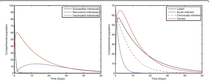
Fig. 1Solution curves of model (1) with respect to the following parameter values and initial size of the compartmental populationb= 0.0121,ξ= 0.8,η= 0.11,β= 0.012,γ= 0.46,ζ= 0.0123,σ= 0.0012,φ= 0.01,ψ = 0.012,v= 0.6,p= 0.6,γ1= 0.33,γ2= 0.009,γ3= 0.025,μ0= 0.069,μ1= 0.000532,μ2= 0.000532,S(0) = 100,

lim

t→∞ sup sup

1

t

Z t

0

ℓð ÞB dt<−2μ₀<0: ð29Þ

From eq. (29), we have

q¼ lim

t→∞ sup sup

1

t

Z t

0

ℓð ÞB dt<0: ð30Þ

Thus, the system containing the first three equations of the model (1) is globally asymptotically stable around its interior equilibrium (S1,L1,A1). Now consider the

sub-system of the model (1), such that

dB tð Þ

dt ¼pγ1A tð Þ−ðμ0þμ1þγ2ÞB tð Þ; dC tð Þ

dt ¼bξηC tð Þ þð1−pÞγ1A tð Þ− μ0þμ2þγ3

C tð Þ;

dR tð Þ

dt ¼ψA tð Þ þγ2B tð Þ þγ3C tð Þ−μ0R tð Þ; dV tð Þ

dt ¼bð1−ξÞ þvS tð Þ−ðμ0þφÞV tð Þ:

ð31Þ

By taking the limit of the system (31), we obtain

0 5 10 15 20

10 15 20 25 30 35 40 45 50 55 60

Time (Months)

Carrier individuals

ξ=0.008 ξ=0.08 ξ=0.8

0 5 10 15 20

0 2 4 6 8 10 12 14

Time (Months)

Recovered individual

s

ξ=0.008 ξ=0.08 ξ=0.8

0 5 10 15 20

10 15 20 25 30 35 40 45 50 55

Time (Months)

Vaccinated individuals

ξ=0.008 ξ=0.08 ξ=0.8

0 5 10 15 20

0 10 20 30 40 50 60 70

Time (Months)

Latant individuals

ξ=0.008 ξ=0.08 ξ=0.8

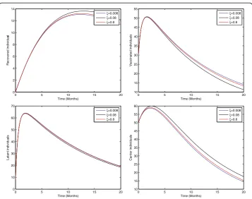
Fig. 2Sensitivity analysis of model (1) by varying the value ofξ= 0.008, 0.08, 0.8 with all other values fixed: b= 0.0121,η= 0.11,β= 0.012,γ= 0.46,ζ= 0.0123,σ= 0.0012,φ= 0.01,ψ= 0.012,v= 0.6,p= 0.6,γ1= 0.33,γ2

= 0.009,γ3= 0.025,μ0= 0.069,μ1= 0.000532,μ2= 0.000532,S(0) = 100,A(0) = 70,B(0) = 60,C(0) = 50,R(0) = 0,

dB tð Þ

dt ¼pγ1A1−ðμ0þμ1þγ2ÞB tð Þ; dC tð Þ

dt ¼bξηC tð Þ þð1−pÞγ1A1− μ0þμ2þγ3

C tð Þ;

dR tð Þ

dt ¼ψA1þγ2B1þγ3C1−μ0R tð Þ; dV tð Þ

dt ¼bð1−ξÞ þvS1−ðμ0þφÞV tð Þ:

ð32Þ

This solves the system (32) using the initial conditions B(0), C(0), R(0), and V(0). Thus, for large time t, that is, t→∞, B(t)→B1, C(t)→C1, R(t)→R1, and V(t)→V1,

which is sufficient to prove that the endemic equilibrium point E1is globally

asymptot-ically stable.

Results and discussions

Numerical results and discussion

In this section, the numerical simulations of the proposed model (1) are presented. The numerical results are obtained by using the fourth-order Runge–Kutta scheme [9, 10]. The simulation of our paper should be considered from a qualitative point of view, but not from the quantitative point of view. Therefore, for this purpose, some of the pa-rameters are taken from published articles and some are assumed with feasible values.

0 5 10 15 20

10 15 20 25 30 35 40 45 50 55 60

Time (Months)

Carrier individuals

η=0.001 η=0.2 η=0.8

0 5 10 15 20

0 2 4 6 8 10 12 14

Time (Months)

Recoverd individuals

η=0.001 η=0.2 η=0.8

0 5 10 15 20

10 15 20 25 30 35 40 45 50 55

Time (Months)

Vaccinated individuals

η=0.001 η=0.2 η=0.8

0 5 10 15 20

0 10 20 30 40 50 60 70

Time (Months)

Latant individuals

η=0.001 η=0.2 η=0.8

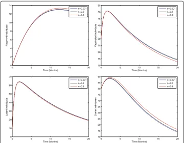
Fig. 3Sensitivity analysis of model (1) by varying the value ofη= 0.001, 0.2, 0.8 with all other parameters fixed:b= 0.0121,ξ= 0.8β= 0.012,γ= 0.46,ζ= 0.0123,σ= 0.0012,φ= 0.01,ψ= 0.012,v= 0.6,p= 0.6,γ1= 0.33,

γ2= 0.009,γ3= 0.025,μ0= 0.069,μ1= 0.000532,μ2= 0.000532,S(0) = 100,A(0) = 70,B(0) = 60,C(0) = 50,R(0) =

For our simulation, we consider the parameter values as follows:b= 0.0121,ξ= 0.8,η= 0.11, β= 0.012, γ= 0.46, ζ= 0.0123, σ= 0.0012, φ= 0.01, ψ= 0.012,v= 0.6,p= 0.6,γ1=

0.33, γ2= 0.009, γ3= 0.025, μ0= 0.069, μ1= 0.000532, and μ2= 0.000532. Some of these

parameters, the birth rate b, natural death rate μ0, and proportion of perinatally

in-fected individuals η, are taken from [13, 21, 22] and the remaining parameters are as-sumed with biologically feasible values.

Fig. 1 represents the dynamical behavior of susceptible, recovered, vaccinated, latent, acute infected, chronically infected, and vaccinated individuals, respectively. Moreover, the time interval is taken 0–50, while the initial population size for the compartmental population susceptible, latent, acute infected, chronically infected, carriers, recovered, and vaccinated individuals are taken to be 100, 10, 70, 60, 50, 0, and 30, respectively. The simulation of our proposed model shows that the susceptible, acute infected, and chronically infected individuals decrease sharply, while the latent, carrier recovered, and vaccinated increase at the beginning and then decrease, as shown in Fig. 1.

Sensitivity analysis

In the study of biological dynamics, the transmission dynamics of infectious disease sensitivity analysis play an especially important role. Using sensitivity analysis, we can investigate the role of each parameter used in the model and can easily develop a strat-egy to control the spread of infection in the community. To do this, local sensitivity analysis of the proposed model (1) has been carried out by varying parameters such as

0 5 10 15 20

0 10 20 30 40 50 60 70 80 90 100

Time (Months)

Susceptible Individuals

β=0.0012 β=0.012 β=0.12

0 5 10 15 20

0 10 20 30 40 50 60 70 80

Time (Months)

Vaccinated individuals

β=0.0012 β=0.012 β=0.12

0 5 10 15 20

0 20 40 60 80 100 120

Time (Months)

Latant individuals

β=0.0012 β=0.012 β=0.12

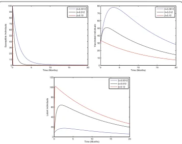
Fig. 4Sensitivity analysis of model (1) by varying the value of_β= 0.0012, 0.012, 0.12 with all other

parameters fixed:_b= 0.0121,_η= 0.8,_ξ= 0.8,_γ= 0.46,_ζ= 0.0123,_σ= 0.0012,_φ= 0.01,_ψ= 0.012,_v= 0.6,_p= 0.6, γ1= 0.33,γ2= 0.009,γ3= 0.025,μ0= 0.069,μ1= 0.000532,μ2= 0.000532,S(0) = 100,A(0) = 70,B(0) = 60,C(0) =

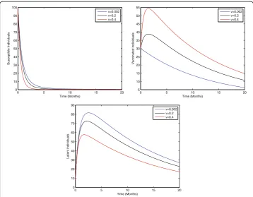
the birth rate, birth rate without successful vaccination, proportion of perinatally in-fected individuals, interaction rate of inin-fected and susceptible individuals, vaccination, and the average probability of those individuals who fail to recover in acute stage and develop the chronic stage. Thus, Figs 2–5 represents the sensitivity analysis of our pro-posed model (1) with respect to birth rate without successful vaccination, proportion of perinatally infected individuals, the interaction rate of susceptible and infected individ-uals, and vaccination.

Figure 2 shows that the birth rate without successful vaccination is directly propor-tional to carrier and inversely proporpropor-tional to susceptible and vaccinated individuals, while having no impact on acute and chronically infected individuals, which shows that the inflow of newborns without successful vaccination will increase the risk of carrier individuals. Fig. 3 represents that the rate of perinatally infected individuals is directly proportional to carrier and inversely proportional to latent and vaccinated individuals, while it has no impact on susceptible, acute infected, or and chronically infected indi-viduals. Similarly to the inflow of newborns without successful vaccination, perinatally infected individuals will also increase the risk of the carrier population. Fig. 4 shows that the transmission/contact rate is directly proportional to the number of infected in-dividuals including the latent, acute infected, chronically infected, and carrier individ-uals, while inversely proportional susceptible, recovered, and vaccinated individindivid-uals, which shows that the increasing contact rate of infected and non-infected will increase the risk of the infected population. Fig. 5 shows that the vaccination rate is directly pro-portional to recovered and vaccinated individuals and inversely propro-portional to

0 5 10 15 20

0 10 20 30 40 50 60 70 80 90 100

Time (Months)

Susceptible Individuals

v=0.002 v=0.2 v=0.4

0 5 10 15 20

5 10 15 20 25 30 35 40 45 50 55

Time (Months)

Vaccinated individuals

v=0.002 v=0.2 v=0.4

0 5 10 15 20

0 10 20 30 40 50 60 70 80 90

Time (Months)

Latant individuals

v=0.002 v=0.2 v=0.4

Fig. 5Sensitivity analysis of model (1) by varying the value ofv= 0.002, 0.2, 0.4 with all other parameters fixed:b= 0.0121,ξ= 0.8,η= 0.8,β= 0.012,γ= 0.46,ζ= 0.0123,σ= 0.0012,φ= 0.01,ψ= 0.012,p= 0.6,γ1=

0.33,γ2= 0.009,γ3= 0.025,μ0= 0.069,μ1= 0.000532,μ2= 0.000532,S(0) = 100,A(0) = 70,B(0) = 60,C(0) = 50,

susceptible and latent individuals, which illustrates that increasing vaccination will de-crease the risk of an infected population. Thus, from the above discussion it is clear that for the control of hepatitis B, we need to pay more attention to the above risk factors.

Conclusion

In this article, we established a model for the transmission dynamics of hepatitis B by taking into account the classification of different phases of individuals infected with hepatitis B. We studied different mathematical analyses, including equilibrium analysis and boundedness, and obtained the basic reproduction number by using the next-generation matrix. Moreover, we discussed the stability analysis and showed that the established model is both locally as well as globally asymptotically stable for the pos-sible equilibria. To discuss the local stability, linearization and Routh—Herwitz criteria were used, while global stability was retrieved by using the method of Castillo-Chávez et al. and a geometrical approach. Finally, the numerical simulation and sensitivity ana-lysis were presented to show the feasibility of the proposed work. Our work provides a coherent platform for studying the full dynamics of hepatitis B and an effective direc-tion for theoretical work. The techniques used in this article are also applicable to other epidemic models.

Acknowledgements

The authors would like to thank the anonymous reviewers for their valuable comments.

Funding

This work has been partially supported by the Higher Education Commission (HEC) of Pakistan under project No. 20_– 1983/R, D/HEC/11 and the Basic Science Research Program through the National Research Foundation of Korea (NRF) funded by the Ministry of Education (NRF-2015R1D1A1A02062131).

Availability of data and materials Not applicable.

Authors’contributions

TK and GZ developed the model and showed the local as well as the global stability of the proposed model, while AK and IH Jung derived the numerical simulation of the proposed model. All authors read and approved the final manuscript.

Ethics approval and consent to participate Not applicable.

Consent for publication Not applicable.

Competing interests

The authors declare that they have no competing interests.

Publisher’s Note

Springer Nature remains neutral with regard to jurisdictional claims in published maps and institutional affiliations.

Author details

1_{Department of Mathematics, University of Malakand, Khyber Pakhtunkhawa, Chakdara Dir Lower, Pakistan.} 2_{Department of Mathematics, Pusan National University, Busan 46241, South Korea.}3_{Department of Mathematics,} University of Swat, Mingora, Swat, Khyber Pakhtunkhawa, Pakistan.

Received: 31 May 2016 Accepted: 10 October 2017

References

1. WHO. Hepatitis B. Fact Sheet N°204. http://www.who.int/mediacentre/factsheets/fs204/en/. Accessed 30 Apr 2014. 2. Shepard CW, Finelli L, Bell BP. Hepatitis B virus infection: epidemiology and vaccination. Epidemiol Rev.

3. Mann J, Roberts M. Modelling the epidemiology of hepatitis B in New Zealand. J Theor Biol. 2011;269:266–72. 4. Lavanchy D. Hepatitis B virus epidemiology, disease burden, treatment, and current and emerging prevention and

control measures. J Vir Hep. 2004;11:97–107.

5. Lok AS, Heathcote EJ, Hoofnagle JH. Management of hepatitis B, 2000 summary of a workshop. Gastroen. 2001; 120:1828–53.

6. McMahon BJ. Epidemiology and natural history of hepatitis B. Semin Liver Dis. 2005;25:3–8. 7. Chang MH. Hepatitis virus infection. Semen Fetal Neonatal Med. 2007;12:160–7.

8. Thornley S, Bullen C, Roberts M. Hepatitis B in a high prevalence New Zealand population a mathematical model applied to infection control policy. J Theor Biol. 2008;254:599–603.

9. Zaman G, Kang YH, Jung IH. Stability and optimal vaccination of an SIR epidemic model. BioSys. 2008;93:240–9. 10. Zaman G, Kang YH, Jung IH. Optimal treatment of an SIR epidemic model with time delay. Biosys. 2009;98:43–50. 11. Anderson RM, May RM. Infectious disease of humans. Dynamics and control. Oxford UK: Oxford University Press; 1991. 12. Zhao SJ, Xu ZY, Lu Y. A mathematical model of hepatitis B virus transmission and its application for vaccination

strategy in China. Intern J Epidemiol. 2000;29:744–52.

13. Zou L, Zhang W, Ruan S. Modeling the transmission dynamics and control of hepatitis B virus in China. J Theor Biol. 2010;262:330–8.

14. Khan T, Zaman G, Chohan M. The transmission dynamic and optimal control of acute and chronic hepatitis B. J Biol Dynamic. 2016;11:172–89.

15. Castillo-Chavez C, Yakubu A-A. Mathematical Approaches for Emerging and Re-emerging Infectious Diseases: An Introduction (IMA vol 125). Berlin: Springer; 2002. pp. 153–63.

16. Birkoff, Rota GC. Ordinary Differential Equation. Ginn Boston. 1982.

17. Driessche PVD, Watmough J. Reproduction number and sub-threshold endemic equilibria for compartmental models of disease transmission. Math Biosci. 2002;180

18. Brauer F, van den Driessche P, Wu J, editors. Mathematical epidemiology. Berlin: Springer-Verlag; 2008. 19. Li MY, Muldowney JS. A geometric approach to global stability problems. SIAM J Math Anal Appl. 1996;27:1070–83. 20. Martin JR. Logarithmic norms and projections applied to linear differential system. J Math Anal Appl. 1974;45:4332–454. 21. Zou L, Ruan S, Zhang W. On the sexual transmission dynamic of hepatitis B virus in China. J Theor Biol. 2015;369:1–12. 22. Edmunds WJ, Medley GF, Nokes DJ. The transmission dynamics and control of hepatitis B virus in the Gambia.

Stat Med. 1996;15:2215–33.

• We accept pre-submission inquiries

• Our selector tool helps you to find the most relevant journal

• We provide round the clock customer support

• Convenient online submission

• Thorough peer review

• Inclusion in PubMed and all major indexing services

• Maximum visibility for your research

Submit your manuscript at www.biomedcentral.com/submit