Estimating Linear Models for Compositional Distributional Semantics
Fabio Massimo Zanzotto1
(1) Department of Computer Science University of Rome “Tor Vergata”
Ioannis Korkontzelos Department of Computer Science
University of York [email protected]
Francesca Fallucchi1,2
(2) Universit`a Telematica “G. Marconi”
Suresh Manandhar Department of Computer Science
University of York [email protected]
Abstract
In distributional semantics studies, there is a growing attention in compositionally determining the distributional meaning of word sequences. Yet, compositional dis-tributional models depend on a large set of parameters that have not been explored. In this paper we propose a novel approach to estimate parameters for a class of com-positional distributional models: the addi-tive models. Our approach leverages on two main ideas. Firstly, a novel idea for extracting compositional distributional se-mantics examples. Secondly, an estima-tion method based on regression models for multiple dependent variables. Experi-ments demonstrate that our approach out-performs existing methods for determin-ing a good model for compositional dis-tributional semantics.
1 Introduction
Lexical distributional semantics has been largely used to model word meaning in many fields as computational linguistics (McCarthy and Carroll, 2003; Manning et al., 2008), linguistics (Harris, 1964), corpus linguistics (Firth, 1957), and cogni-tive research (Miller and Charles, 1991). The fun-damental hypothesis is the distributional hypoth-esis (DH): “similar words share similar contexts” (Harris, 1964). Recently, this hypothesis has been operationally defined in many ways in the fields of
physicology, computational linguistics, and infor-mation retrieval (Li et al., 2000; Pado and Lapata, 2007; Deerwester et al., 1990).
Given the successful application to words, dis-tributional semantics has been extended to word sequences. This has happened in two ways: (1) via the reformulation of DH for specific word se-quences (Lin and Pantel, 2001); and (2) via the definition of compositional distributional seman-tics (CDS) models (Mitchell and Lapata, 2008; Jones and Mewhort, 2007). These are two differ-ent ways of addressing the problem.
Lin and Pantel (2001) propose thepattern dis-tributional hypothesis that extends the distribu-tional hypothesis for specific patterns, i.e. word sequences representing partial verb phrases. Dis-tributional meaning for these patterns is derived directly by looking to their occurrences in a cor-pus. Due to data sparsity, patterns of different length appear with very different frequencies in the corpus, affecting their statistics detrimentally. On the other hand, compositional distributional semantics (CDS) propose to obtain distributional meaning for sequences by composing the vectors of the words in the sequences (Mitchell and Lata, 2008; Jones and Mewhort, 2007). This ap-proach is fairly interesting as the distributional meaning of sequences of different length is ob-tained by composing distributional vectors of sin-gle words. Yet, many of these approaches have a large number of parameters that cannot be easily estimated.
es-timate parameters for additive compositional dis-tributional semantics models. Our approach lever-ages on two main ideas. Firstly, a novel way for extracting compositional distributional semantics examples and counter-examples. Secondly, an es-timation model that exploits these examples and determines an equation system that represents a regression problem with multiple dependent vari-ables. We propose a method to estimate a solu-tion of this equasolu-tion system based on the Moore-Penrose pseudo-inverse matrices (Moore-Penrose, 1955). The rest of the paper is organised as follows: Firstly, we shortly review existing compositional distributional semantics (CDS) models (Sec. 2). Then we describe our model for estimating CDS models parameters (Sec. 3). In succession, we introduce a way to extract compositional dis-tributional semantics examples from dictionaries (Sec. 4). Then, we discuss the experimental set up and the results of our linear CDS model with es-timated parameters with respect to existing CDS models (Sec. 5).
2 Models for compositional distributional semantics (CDS)
A CDS model is a functionthat computes the distributional vector of a sequence of wordssby combining the distributional vectors of its com-ponent wordsw1. . .wn. Let(s)be the
distribu-tional vector describingsandw~ithe distributional vectors describing its component wordwi. Then, the CDS model can be written as:
(s) =(w1. . .wn) =w~1. . .w~n (1)
This generic model has been fairly studied and many different functions have been proposed and tested.
Mitchell and Lapata (2008) propose the fol-lowing general CDS model for 2-word sequences
s=xy:
(s) =(xy) =f(~x, ~y, R, K) (2)
where~xand~y are respectively the distributional
vectors of x andy, R is the particular syntactic and/or semantic relation connectingxandy, and,
K represents the amount of background
knowl-edge that the vector composition process takes
vector dimensions
between gap processsocialtwo
contact <11, 0, 3, 0, 11> x:close <27, 3, 2, 5, 24> y:interaction <23, 0, 3, 8, 4>
Table 1: Example of distributional frequency vectors for the triple t = (contact, ~~ close,interaction)~
into account. Two specialisations of the gen-eral CDS model are proposed: thebasic additive
model and thebasic multiplicativemodel. Thebasic additivemodel (BAM) is written as:
(s) =α~x+β~y (3)
where α and β are two scalar parameters. The
simplistic parametrisation is α = β = 1. For
example, given the vectors ~x and ~y of Table 1, BAM(s) =<50,3,5,13,28>.
Thebasic multiplicativemodel (BMM) is writ-ten as:
si =xiyi (4)
where si, xi, and yi are the i-th dimensions of the vectors (s), ~x, and ~y, respectively. For
the example of Table 1, BM M(s) =< 621,0,
6,40,96>.
Erk and Pad´o (2008) look at the problem in a different way. Let the general distributional mean-ing of the wordwbew~. Their model computes a
different vectorw~sthat represents the specific
dis-tributional meaning ofwwith respect tos, i.e.:
~
ws=(w,s) (5)
In general, this operator gives different vectors for each wordwi in the sequences, i.e.(wi,s) 6= (wj,s)ifi 6= j. It also gives different vectors for a wordwiappearing in different sequencessk andsl, i.e.(wi,sk)6=(wi,sl)ifk6=l.
The model of Erk and Pad´o (2008) was de-signed to disambiguate the distributional mean-ing of a word w in the context of the sequence
word that is governing the sequence (c.f. Pollard and Sag (1994)). For example, the distributional meaning of the word sequence eats miceis gov-erned by the verbeats. Following this model, the distributional vector(s)can be written as:
(s)≈ (h,s) (6)
The function (h,s) explicitly uses the
re-lation R and the knowledge K of the general
equation 2, being based on the notion of selec-tional preferences. We exploit the model for se-quences of two wordss=xywhere the two words are related with an oriented syntactic relation r
(e.g. r=adj modifier). For making the
syntac-tic relation explicit, we indicate the sequence as:
s=x←−r y.
Given a word w, the model has to keep track of its selectional preferences. Consequently, each wordwis represented with a triple:
(w, R~ w, R−w1) (7)
wherew~is the distributional vector of the wordw, Rwis the set of the vectors representing the direct selectional preferences of the wordw, andR−w1is
the set of the vectors representing the indirect se-lectional preferences of the wordw. Given a set of syntactic relationsR, the setRwandR−w1contain
respectively a selectional preference vectorRw(r)
andRw(r)−1for eachr ∈ R. Selectional
prefer-ences are computed as in Erk (2007). If xis the semantic head of sequences, then the model can be written as:
(s) =(x,x←−r y) =~xRy(r) (8)
Otherwise, ifyis the semantic head:
(s) =(y,x←−r y) =~yRx−1(r) (9)
is in both cases realised using BAM or BMM. We will call these models: basic additivemodel with selectional preferences (BAM-SP) and basic multiplicative model with selectional preferences (BMM-SP).
Both Mitchell and Lapata (2008) and Erk and Pad´o (2008) experimented with few empirically estimated parameters. Thus, the general additive CDS model has not been adequately explored.
3 Estimating Additive Compositional Semantics Models from Data
The generic additive model sums the vectors ~x
and~yin a new vector~z:
(s) =~z=A~x+B~y (10)
where A andB are two square matrices
captur-ing the relationRand the background knowledge K of equation 2. Writing matrices A and B by
hand is impossible because of their large size. Es-timating these matrices is neither a simple classi-fication learning problem nor a simple regression problem. It is a regression problem with multiple dependent variables. In this section, we propose our model to solve this regression problem using a set of training examplesE.
The set of training examplesEcontains triples
of vectors(~z, ~x, ~y). ~xand~y are the two
distribu-tional vectors of the wordsxandy. ~z is the ex-pected distributional vector of the composition of
~xand~y. Note that for an ideal perfectly
perform-ing CDS model we can write~z = (xy). How-ever, in general the expected vector~zis not
guar-anteed to be equal to the composed one (xy).
Figure 1 reports an example of these triples, i.e.,
t = (contact, ~~ close,interaction)~ , with the
re-lated distributional vectors. The construction of
Eis discussed in section 4.
In the rest of the section, we describe how the regression problem with multiple dependent vari-ables can be solved with a linear equation system and we give a possible solution of this equation system. In the experimental section, we refer to our model as the estimated additive model (EAM).
3.1 Setting the linear equation system
The matrices A and B of equation 10 can be
joined in a single matrix:
~z= A B
~x ~y
(11)
For the tripletof table 1, equation 11 is:
~
contact= A B close~~ interaction
!
and it can be rewritten as:
Focusing on matrix AB, we can transpose the
matrices as follows:
Equation 14 is the prototype of our final equa-tion system. The larger the matrix AB to be estimated, the more equations like 14 are needed. Given set E that contains ntriples (~z, ~x, ~y), we
can write the following system of equations:
The vectors derived from the triples can be seen as two matrices ofnrows,Zand XYrelated to~zT
i and ~xTi ~yTi , respectively. The overall equation
system is then the following:
Z = X Y
This equation system represents the constraints that matricesAandB have to satisfy in order to
be a possible linear CDS model that can at least describe seen examples. We will hereafter call
Λ = A B andQ = X Y. The system
in equation 16 can be simplified as:
Z=QΛT (17)
AsQis a rectangular and singular matrix, it is
not invertible and the system in equation 16 has
no solutions. It is possible to use the principle of Least Square Estimation for computing an ap-proximation solution. The idea is to compute the solutionΛbthat minimises the residual norm, i.e.:
b
ΛT = arg min
ΛT kQΛ
T −Zk2 (18)
One solution for this problem is the Moore-Penrose pseudoinverseQ+ (Penrose, 1955) that
gives the following final equation: b
ΛT =Q+Z (19)
In the next section, we discuss how the Moore-Penrose pseudoinverseis obtained using singular value decomposition (SVD).
3.2 Computing the pseudo-inverse matrix
The pseudo-inverse matrix can provide an approx-imated solution even if the equation system has no solutions. We here compute theMoore-Penrose pseudoinverse using singular value decomposi-tion (SVD) that is widely used in computadecomposi-tional linguistics and information retrieval for reducing spaces (Deerwester et al., 1990).
Moore-Penrose pseudoinverse (Penrose, 1955) is computed in the following way. Let the original matrixQhavenrows and mcolumns and be of
rank r. The SVD decomposition of the original
matrixQisQ = UΣVT whereΣis a square
di-agonal matrix of dimensionr. Then, the
pseudo-inverse matrix that minimises the equation 18 is:
Q+ =VΣ+UT (20)
where the diagonal matrixΣ+is ther×r
trans-posed matrix ofΣhaving as diagonal elements the
reciprocals of the singular values 1
δ1,
Using SVD to compute the pseudo-inverse ma-trix allows for different approximations (Fallucchi and Zanzotto, 2009). The algorithm for comput-ing the scomput-ingular value decomposition is iterative (Golub and Kahan, 1965). Firstly derived dimen-sions have higher singular value. Then, dimension
kis more informative than dimensionk0 > k. We
can consider different values forkto obtain differ-ent SVD for the approximationsQ+k of the
origi-nal matrixQ+in equation 20), i.e.:
whereQ+k is a matrixnbym obtained
consider-ing the firstksingular values.
4 Building positive and negative examples
As explained in the previous section, estimating CDS models, needs a set of triples E, similar to
tripletof table 1. This setEshould contain
pos-itive examples in the form of triples (~zi, ~xi, ~yi). Examples are positive in the sense that ~zi = (xy) for an ideal CDS. There are no available
sets to contain such triples, with the exception of the set used in Mitchell and Lapata (2008) which is designed only for testing purposes. It contains similar and dissimilar pairs of sequences (s1,s2)
where each sequence is a verb-noun pair (vi,ni). From the positive part of this set, we can only de-rive quadruples where (v1n1) ≈ (v2n2) but
we cannot derive the ideal resulting vector of the composition (vini). Sets used to test multi-word expression (MWE) detection models (e.g., (Schone and Jurafsky, 2001; Nicholson and Bald-win, 2008; Kim and BaldBald-win, 2008; Cook et al., 2008; Villavicencio, 2003; Korkontzelos and Manandhar, 2009)) are again not useful as con-taining only valid MWE that cannot be used to determine the set of training triples needed here.
As a result, we need a novel idea to build sets of triples to train CDS models. We can leverage on knowledge stored in dictionaries. In the rest of the section, we describe how we build the positive example setEand a control negative example set N E. Elements of the two sets are pairs (t,s) where tis a target wordsis a sequence of words.tis the word that represent the distributional meaning of
sin the case ofE. Contrarily,tis totally unrelated
to the distributional meaning ofsinN E. The sets E andN E can be used both for training and for
testing. In the testing phase, we can use these sets to determine whether a CDS model is good or not and to compare different CDS models.
4.1 Building Positive Examples using Dictionaries
Dictionariesas natural repositories of equivalent expressions can be used to extract positive exam-ples for training and testing CDS models. The basic idea is the following: dictionary entries are
declarationsof equivalence. Words or, occasion-ally, multi-word expressionstare declared to be semantically similar to their definition sequences
s. This happens at least for some sense of the defined words. We can then observe thatt ≈ s. For example, we report some sample definitions ofcontactandhigh life:
target word (t) definition sequence (s)
contact close interaction
high life excessive spending
In the first case, a word, i.e.contact, is semanti-cally similar to a two-word expression, i.e.close interaction. In the second case, two two-word ex-pressions are semantically similar.
Then, the pairs (t,s) can be used to model
positive cases of compositional distributional se-mantics as we know that the word sequence s
is compositional and it describes the meaning of the wordt. The distributional meaning~toft is the expected distributional meaning ofs. Conse-quently, the vector~tis what the CDS model(s)
should compositionally obtain from the vectors of the componentss~1 . . .s~m ofs. This way of ex-tracting similar expressions has some interesting properties:
First property Defined words t are generally single words. Thus, we can extract stable and meaningful distributional vectors for these words and then compare them to the distributional vec-tors composed by CDS model. This is an impor-tant property as we cannot compare directly the distributional vector~sof a word sequence sand
the vector(s) obtained by composing its
com-ponents. As the word sequencesgrows in length, the reliability of the vector~s decreases since the
sequencesbecomes rarer.
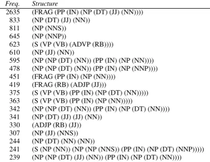
Second property Definitionsshave a large va-riety of different syntactic structures ranging from simple structures as Adjective-Noun to more com-plex ones. This gives the possibility to train and test CDS models that take into account syntax. Table 2 represents the distribution of the more frequent syntactic structures in the definitions of WordNet1(Miller, 1995).
1Definitions were extracted from WordNet 3.0 and were
Freq. Structure
2635 (FRAG (PP (IN) (NP (DT) (JJ) (NN)))) 833 (NP (DT) (JJ) (NN))
811 (NP (NNS)) 645 (NP (NNP))
623 (S (VP (VB) (ADVP (RB)))) 610 (NP (JJ) (NN))
595 (NP (NP (DT) (NN)) (PP (IN) (NP (NN)))) 478 (NP (NP (DT) (NN)) (PP (IN) (NP (NNP)))) 451 (FRAG (PP (IN) (NP (NN))))
419 (FRAG (RB) (ADJP (JJ)))
375 (S (VP (VB) (PP (IN) (NP (DT) (NN))))) 363 (S (VP (VB) (PP (IN) (NP (NN)))))
342 (NP (NP (DT) (NN)) (PP (IN) (NP (DT) (NN)))) 341 (NP (DT) (JJ) (JJ) (NN))
330 (ADJP (RB) (JJ)) 307 (NP (JJ) (NNS)) 244 (NP (DT) (NN) (NN))
241 (S (NP (NN)) (NP (NP (NNS)) (PP (IN) (NP (DT) (NNP))))) 239 (NP (NP (DT) (JJ) (NN)) (PP (IN) (NP (DT) (NN))))
Table 2: Top 20 syntactic structures of WordNet definitions
4.2 Extracting Negative Examples from Word Etymology
In order to devise complete training and testing sets for CDS models, we need to find a sensible way to extract negative examples. An option is to randomly generate totally unrelated triples for the negative examples set, N E. In this case, due to
data sparsenessN E would mostly contain triples
(~z, ~x, ~y)where it is expected that~z6=(xy). Yet,
these can be too generic and too loosely related to be interesting cases.
Instead we attempt to extract sets of negative pairs (t,s) comparable with the one used for build-ing the trainbuild-ing setE. The target word tshould
be a single word and s should be a sequence of words. The latter should be a sequence of words related by construction tot but the meaning oft
andsshould be unrelated.
The idea is the following: many words are et-ymologically derived from very old or ancient words. These words represent a collocation which is in general not related to the meaning of the target word. For example, the word philosophy
derives from two Greek words philos (beloved) and sophia (wisdom). However, the use of the word philosophyin not related to the collocation
beloved wisdom. This word has lost its origi-nal compositioorigi-nal meaning. The following table shows some more etymologically complex words along with the compositionally unrelated colloca-tions:
target word compositionally unrelated seq.
municipal receive duty
octopus eight foot
As the examples suggest, we are able to build a set N E with features similar to the features of N. In particular, each target word is paired with a related word sequence derived from its etymol-ogy. These etymologically complex words are un-related to the corresponding compositional collo-cations. To derive a setN Ewith the above
char-acteristics we can use dictionaries containing ety-mological information as Wiktionary2.
5 Experimental evaluation
In the previous sections, we presented the esti-mated additive model (EAM): our approach to es-timate the parameters of a generic additive model for CDS. In this section, we experiment with this model to determine whether it performs better than existing models: the basic additive model (BAM), the basic multiplicative model (BMM), the basic additive model with selectional pref-erences (BAM-SP), and the basic multiplicative model with selectional preferences (BMM-SP) (c.f. Sec. 2). In succession, we explore whether our estimated additive model (EAM) is better than any possible BAM obtained with parameter ad-justment. In the rest of the section, we firstly give the experimental setup and then we discuss the ex-periments and the results.
5.1 Experimental setup
Our experiments aim to compare compositional distributional semantic (CDS) modelswith re-spect to their ability of detecting statistically sig-nificant difference between sets E and N E. In particular, the average similarity sim(~z,(xy))
for(~z, ~x, ~y) ∈E should be significantly different
fromsim(~z,(xy))for(~z, ~x, ~y) ∈ N E. In this section, we describe the chosen similarity mea-suresim, statistical significance testing and
con-struction details for the training and testing set. Cosine similarity was used to compare the con-text vector~z representing the target wordz with
the composed vector(xy)representing the
con-text vector of sequencex y. Cosine similarity
tween two vectors~xand~yof the same dimension
is defined as:
sim(~x, ~y) = ~x·~y
k~xk k~yk (22)
where·is the dot product andk~ak is the magni-tude of vector~acomputed the Euclidean norm.
To evaluate whether a CDS model distinguishes positive examples E from negative examples N E, we test if the distribution of similarities sim(~z,(xy)) for (~z, ~x, ~y) ∈ E is statistically
different from the distribution of the same simi-larities for (~z, ~x, ~y) ∈ N E. For this purpose, we
used Student’s t-test for two independent samples of different sizes. t-test assumes that the two dis-tributions are Gaussian and determines the prob-ability that they are similar, i.e., derive from the same underlying distribution. Low probabilities indicate that the distributions are highly dissimilar and that the corresponding CDS model performs well, as it detects statistically different similarities for the positive setEand the negative setN E.
Based on the null hypothesis that the means of the two samples are equal, µ1 =µ2, Student’s
t-test takes into account the sizesN, meansM and
variances s2 of the two samples to compute the
following value:
t= (M1−M2)−1
s
2(s2 1+s22)
df∗Nh (23)
wheredf =N1 +N2−2stands for the degrees
of freedom and Nh = 2(N1−1 +N2−1)−1 is the
harmonic mean of the sample sizes. Given the statistictand the degrees of freedomdf, we can
compute the correspondingp-value, i.e., the
prob-ability that the two samples derive from the same distribution. The null hypothesis can be rejected if thep-value is below the chosen threshold of
statis-tical significance (usually0.1,0.05or0.01),
oth-erwise it is accepted. In our case, rejecting the null hypothesis means that the similarity values of instances ofEare significantly different from
in-stances of N E, and that the corresponding CDS
model perform well.p-value can be used as a
per-formance ranking function for CDS models. We constructed two sets of instances: (a) a set containing Adjective-Noun or Noun-Noun
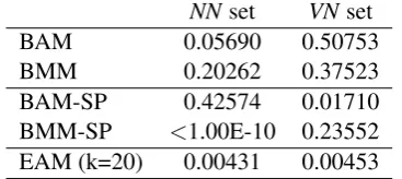
se-NNset VNset
BAM 0.05690 0.50753
BMM 0.20262 0.37523
BAM-SP 0.42574 0.01710 BMM-SP <1.00E-10 0.23552
EAM (k=20) 0.00431 0.00453 Table 3: Probability of confusingEandN Ewith
different CDS models
quences (NN set); and (b) a set containing Verb-Noun sequences (VN set). Capturing different syntactic relations, these two sets can support that our results are independent from the syntactic re-lation between the words of each sequence. For each set, we used WordNet for extracting positive examplesE and Wiktionary for extracting
nega-tive examplesN Eas described in Section 4. We
obtained the following sets: (a) NN consists of
1065word-sequence pairs from WordNet
defini-tions and 377 pairs extracted from Wiktionary;
and (b) VN consists of 161 word-sequence pairs
from WordNet definitions and111pairs extracted
from Wiktionary. We have then divided these two sets in two parts of 50% each, for training and testing. Instances of the training part ofE have
been used to estimate matricesAandBfor model EAM, while the testing parts have been used for
testing all models. Frequency vectors for all sin-gle words occurring in the above pairs were con-structed from the British National Corpus using sentences as contextual windows and words as features. The resulting space has 689191 features.
5.2 Results and Analysis
The first set of experiments compares EAM with other existing CDS models: BAM, BMM, BAM-SP, and BMM-SP. Results are shown in Table 3. The table reports thep-value, i.e., the probability of confusing the positive setE and the negative
setN Efor all models. Lower probabilities
char-acterise better models. Probabilities below 0.05 indicate that the model detects a statistically sig-nificant difference between setsEandN E. EAM
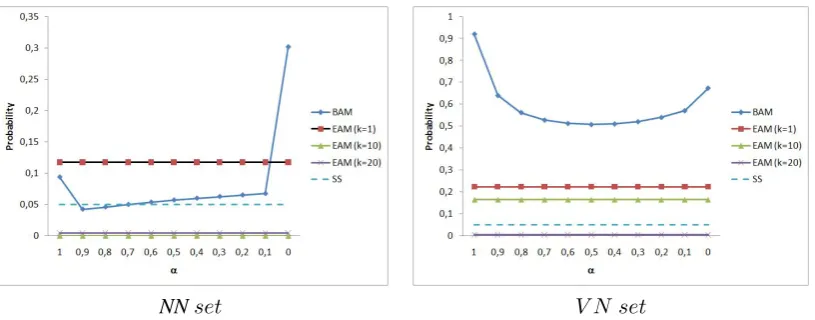
NNset V N set
Figure 1: p-values of BAM with different values for parameterα(whereβ = 1−α) and of EAM for
different approximations of the SVD pseudo-inverse matrix (k)
The first observation is that EAM models sig-nificantly separate positive from negative exam-ples for both sets. This is not the case for any of the other models. Only, the selectional prefer-ences based models in two cases have this prop-erty, but this cannot be generalised: BAM-SP on theVN set and BMM-SP on theNN set. In gen-eral, these models do not offer the possibility of separating positive from negative examples.
In the second set of experiments, we attempt to investigate whether simple parameter adjustment of BAM can perform better than EAM. Results are shown in figure 1. Plots show the basic additive model (BAM) with different values for parameter
α(whereβ = 1−α) and EAM computed for
dif-ferent approximations of the SVD pseudo-inverse matrix (i.e., with different k). The x-axis of the
plots represents parameterαand the y-axis
repre-sents the probability of confusing the positive set
Eand the negative setN E. The representation
fo-cuses on the performance ofBAM with respect to
differentαvalues. The performance of EAM for
different k values is represented with horizontal
lines. Probabilities of different models are directly comparable. Line SS represents the threshold of statistical significance; the value below which the detected difference between the E andN E sets
becomes statistically significant.
Experimental results show some interesting facts: While BAM forα >0perform better than EAM computed with k = 1in the NN set, they
do not perform better in the VN set. EAM with
k = 1 has1 degree of freedom corresponding to
1parameter, the same as BAM. The parameter of
EAM is tuned on the training set, in contrast to
α, the parameter of BAM. Increasing the number
of considered dimensions, k of EAM, estimated
models outperform BAM for all values of param-eterα. Moreover, EAM detect a statistically
sig-nificant difference between theEand theN Esets
fork ≥ 10 andk = 20for theNN set and the VNset set, respectively. Simple parametrisation
of a BAM does not outperform the proposed esti-mated additive model.
6 Conclusions
In this paper, we presented an innovative method to estimate linear compositional distributional se-mantics models. The core of our approach con-sists on two parts: (1) providing a method to es-timate the regression problem with multiple de-pendent variables and (2) providing a training set derived from dictionary definitions. Experiments showed that our model is highly competitive with respect to state-of-the-art models for composi-tional distribucomposi-tional semantics.
References
Charniak, Eugene. 2000. A maximum-entropy-inspired parser. Inproceedings of the 1st NAACL, pages 132–139, Seattle, Washington.
Deerwester, Scott C., Susan T. Dumais, Thomas K. Landauer, George W. Furnas, and Richard A. Harsh-man. 1990. Indexing by latent semantic analysis.
Journal of the American Society of Information Sci-ence, 41(6):391–407.
Erk, Katrin and Sebastian Pad´o. 2008. A structured vector space model for word meaning in context. In
proceedings of the Conference on Empirical Meth-ods in Natural Language Processing, pages 897– 906. Association for Computational Linguistics. Erk, Katrin. 2007. A simple, similarity-based model
for selectional preferences. Inproceedings of ACL. Association for Computer Linguistics.
Fallucchi, Francesca and Fabio Massimo Zanzotto. 2009. SVD feature selection for probabilistic tax-onomy learning. Inproceedings of the Workshop on Geometrical Models of Natural Language Seman-tics, pages 66–73. Association for Computational Linguistics, Athens, Greece.
Firth, John R. 1957. Papers in Linguistics. Oxford University Press, London.
Golub, Gene and William Kahan. 1965. Calculat-ing the sCalculat-ingular values and pseudo-inverse of a ma-trix. Journal of the Society for Industrial and Ap-plied Mathematics, Series B: Numerical Analysis, 2(2):205–224.
Harris, Zellig. 1964. Distributional structure. In Katz, Jerrold J. and Jerry A. Fodor, editors, The Philos-ophy of Linguistics, New York. Oxford University Press.
Jones, Michael N. and Douglas J. K. Mewhort. 2007. Representing word meaning and order information in a composite holographic lexicon. Psychological Review, 114:1–37.
Kim, Su N. and Timothy Baldwin. 2008. Standard-ised evaluation of english noun compound inter-pretation. Inproceedings of the LREC Workshop: Towards a Shared Task for Multiword Expressions (MWE 2008), pages 39–42, Marrakech, Morocco.
Korkontzelos, Ioannis and Suresh Manandhar. 2009. Detecting compositionality in multi-word expres-sions. In proceedings of ACL-IJCNLP 2009, Sin-gapore.
Li, Ping, Curt Burgess, and Kevin Lund. 2000. The acquisition of word meaning through global lexical co-occurrences. In proceedings of the 31st Child Language Research Forum.
Lin, Dekang and Patrick Pantel. 2001. DIRT-discovery of inference rules from text. In Proceed-ings of the ACM Conference on Knowledge Discov-ery and Data Mining (KDD-01). San Francisco, CA.
Manning, Christopher D., Prabhakar Raghavan, and Hinrich Sch¨utze. 2008. Introduction to Information Retrieval. Cambridge University Press, Cambridge, UK.
McCarthy, Diana and John Carroll. 2003. Disam-biguating nouns, verbs, and adjectives using auto-matically acquired selectional preferences. Compu-tational Linguistics, 29(4):639–654.
Miller, George A. and Walter G. Charles. 1991. Con-textual correlates of semantic similarity. Language and Cognitive Processes, VI:1–28.
Miller, George A. 1995. WordNet: A lexical database for English. Communications of the ACM, 38(11):39–41.
Mitchell, Jeff and Mirella Lapata. 2008. Vector-based models of semantic composition. In proceedings of ACL-08: HLT, pages 236–244, Columbus, Ohio. Association for Computational Linguistics.
Nicholson, Jeremy and Timothy Baldwin. 2008. Inter-preting compound nominalisations. Inproceedings of the LREC Workshop: Towards a Shared Task for Multiword Expressions (MWE 2008), pages 43–45, Marrakech, Morocco.
Pado, Sebastian and Mirella Lapata. 2007. Dependency-based construction of semantic space models. Computational Linguistics, 33(2):161– 199.
Penrose, Roger. 1955. A generalized inverse for ma-trices. InProceedings of Cambridge Philosophical Society.
Pollard, Carl J. and Ivan A. Sag. 1994. Head-driven Phrase Structured Grammar. Chicago CSLI, Stan-ford.
Schone, Patrick and Daniel Jurafsky. 2001. Is knowledge-free induction of multiword unit dictio-nary headwords a solved problem? In Lee, Lil-lian and Donna Harman, editors,proceedings of the Conference on Empirical Methods in Natural Lan-guage Processing, pages 100–108.