A Comparative Analysis of Hyperspectral and Multispectral Image Classification Techniques

(1)

ISSN(Online): 2320-9801

ISSN (Print): 2320-9798

I

nternational

J

ournal of

I

nnovative

R

esearch in

C

omputer

and

C

ommunication

E

ngineering

(A High Impact Factor, Monthly, Peer Reviewed Journal) Website: www.ijircce.com

Vol. 5, Issue 10, October 2017

A Comparative Analysis of Hyperspectral and

Multispectral Image Classification Techniques

P.Dolphin Devi1, Dr.K.Chitra2

Assistant Professor, Dept. of C.S., GTN Arts College (Autonomous), Dindigul, Tamilnadu, India1 Assistant Professor, Dept. of C.S., Government Arts College, Melur, Madurai, Tamilnadu, India2

ABSTRACT: In recent years, the use of remote sensing imagery has gained more popularity among the researchers to classify and map vegetation over the large spatial regions. Hyperspectral Image (HSI) and multispectral image play a vital role in the field of remote sensing. Remote sensing is used in numerous applications such as map drawing, disaster management, delimitation of land parcels, land usage planning, agriculture and studies on hydrology and forest. These applications involve the classification of pixels in an image into a number of classes. A wide range of image classification techniques is available based on the spectral and spatial information. This paper presented a comparative analysis of HSI and multispectral image classification techniques along with the advantages. It highlights the latest classification approaches and describes an experimental evaluation of a few major classification algorithms.

KEYWORDS: Classification, Hyperspectral Image (HSI), Multispectral Image, Remote Sensing I. INTRODUCTION

Remote sensing is the process of acquiring information about the earth’s environment using the images acquired by the satellite. The advantage of remote sensing is that the environmental data covering a large surface can be captured instantaneously and processed for generating map [1].

The ability for analyzing the information from the remote sensing satellite enables monitoring of the earth’s surface. The remote sensing data is used for the mapping of vegetation over the large spatial scales. The remote sensing data is available as multispectral image and HSI. In multispectral imaging, the sensors collect image data ranging between three to six spectral bands from the visible and near-infrared region. In hyperspectral imaging, the sensors collect multiple narrow spectral bands from the visible and infrared regions. These sensors collect around 200 or more spectral bands and enable construction of continuous spectral reflectance signature. The HSI data at a finer spectral resolution can be used for effective vegetation classification by detecting the structural differences in vegetation areas [2].

The classification of land cover from the captured image is an emerging research topic in the remote sensing applications. Image classification is the process of automatically categorizing the pixels in the remote sensed image into individual classes. The main objective of the image classification is to identify the features that represent the land cover. The image classification techniques are classified as supervised and unsupervised classifications. In the supervised classification, the spectral features of areas from a satellite dataset are used to form a training dataset. In unsupervised classification, the group of pixels from the image is automatically clustered based on the spectral features. Each cluster is identified as a type of separate land cover. Classification of remote sensed data is a challenging task due to the presence of complex landscape and usage of classification methodology. This paper presented a comparative analysis of HSI and multispectral image classification techniques. An overview of the HSI and multispectral image classification techniques along with the performance analysis is described in this paper.

(2)

ISSN(Online): 2320-9801

ISSN (Print): 2320-9798

I

nternational

J

ournal of

I

nnovative

R

esearch in

C

omputer

and

C

ommunication

E

ngineering

II. IMAGE CLASSIFICATIONAPPROACHES

A.Sparse Logistic Regression (SLR)

SLR selects a few discriminative input variables from the shared feature space for the approximate prediction of the system output [3]. This reduces the distribution shift and increases the classification accuracy. In the training process, the objective function of SLR is minimized as

min , ∑ log 1 + − ( + ) + ‖ ‖ (1)

Where represents the feature vector and ∈{1,−1} represents the class label of the ith training sample. indicates the regularization parameter. The computational complexity of each iteration is ( )[4]. After estimating the coefficients ‘w’ and ‘c’, the classifier operates in a probabilistic manner for labeling the input test sample ‘x’ using the feature vector

( = 1| ) = (2)

For multiclass problem, the one-vs-one voting scheme can be used. The multitask SLR (MTSLR) is used for the simultaneous training of two SLR models with the label samples in the source and target scenes. But, the two SLR models share a common discriminative feature subset. The SLR-based classifier trains a single SLR model for both scenes, the MTSLR provides strongly related and little differentiated classifier for two different scenes. This reduces the impact of residuary distribution shift after adapting the dictionary learning-based feature-level domain. Despite of training two SLR models separately, they are bound together by sharing the same sparse structure in coefficient vectors defined as

‖[ , ]‖ , =∑ ( ) + ( ) (3)

The regularization parameter controls the sparsity level in and . The MTSLR model completes the selection of combined feature and simultaneous training of two classifiers. As the ℓ , norm regularization term in the objective

function cannot be differentiable at certain points, the whole objective function cannot be minimized using the gradient descent [5-7].

B. Multiple-Feature-Based Adaptive Sparse Representation (MFASR)

In the multiple-feature case, a pixel ‘x’ is represented using four features = { } _{, , ,} where is the kth feature vector [8]. The four feature dictionaries set = { } _{, , ,} is created by extracting the pixels from these features. For the pixel of each feature, the sparse coding algorithm is used to obtain the corresponding sparse coefficient . The class label of the test pixel is determined by mutually computing the minimum residual

( ) = arg min ,…, ∑ ‖ − ‖ (4)

(3)

ISSN(Online): 2320-9801

ISSN (Print): 2320-9798

I

nternational

J

ournal of

I

nnovative

R

esearch in

C

omputer

and

C

ommunication

E

ngineering

sparse coefficients are controlled to have a same class-level sparsity pattern and can select different atoms within one class. Hence, desired sparse coefficients for the test pixels of multiple features will have a same class-level pattern and different feature-level pattern.

Each adaptive set is represented as the indexes of non-zero scalar coefficients that belong to the same class in the sparse matrix. The above optimization problem is solved using the adaptive sparse algorithm [9].After obtaining the sparse matrix, the combined residual errors are computed to determine the class to which the pixel belongs to. A spatial window for each pixel is defined for manipulating the spatial information of the HyperSpectral Image (HSI) features. This improves the classification performance. Rather than using a fixed size window, a Shape Adaptive (SA) window is chosen for the pixel of each feature. The pixels within the SA window can create a set matrix { } _{, , ,} where

= [ , , … , ]. The SA sparse matrix for the set matrix is obtained by

= arg min ∑ − . ‖ ‖ , ≤ (5)

Where = [ , , , ]. The = [ , , … , ] is the coefficient matrix associated with the feature ‘k’.

C.Bayesian logistic regression with Super Gaussians

The variational methods are applied for approximating the posterior distribution by ( )[10]. Reduction of the Kullback-Leibler (KL) divergence is the variational criterion. This is used to find ( ),

( ( )‖ ( | )) =∫ ( ) log ( )

( | ) (6)

= +∫ ( ) log _{( | )}( ) (7)

Due to the form of the prior and observation models, the integral cannot be calculated. To solve this problem, a lower bound for the distribution ( | ) is found out with a function that renders the calculation of ( ( )‖ ( | ))

to be possible when ( | ) is replaced by such function.

( )≥ − ∑ − ∗ ₌ _{( , )} ₍₈₎

Where = ( , … , ) and is a constant. To obtain a lower bound on ( | ), the variational bound is applied to the sigmoid function. Then,

log ( | ) =∑ log ≥log ( , , ) (9)

Where log ( , , ) =∑ − − − −log(1 + )

Where = ( , … , ) and ∈ ℝ with = − .

Using the lower bounds in the above equations, the joint distribution is bounded below by

( , )≥ ( , ) ( , , ) = ( , , , ) (10)

( , )is replaced by this lower bound. ( )is a Gaussian distribution with mean and covariance matrix given by

(4)

ISSN(Online): 2320-9801

ISSN (Print): 2320-9798

I

nternational

J

ournal of

I

nnovative

R

esearch in

C

omputer

and

C

ommunication

E

ngineering

〈 〉= ∑ − (12)

With Ξ= diag( ), = 1, … , . The update of auxiliary vectors ξ and is given by

= arg max 〈log ( , , , )〉 ( ) (13)

= arg max 〈log ( , , , )〉 ( ) (14)

All parameters including the distribution of the adaptive coefficients are estimated. The estimates of the adaptive coefficient vector are given by 〈 〉. If a new sample ∗ is given, it is utilized as predictive distribution of the classes

( | ∗_{) =}

〈 〉 ∗ (15)

( | ∗_{) = 1}₋ _{( |} ∗₎ ₍₁₆₎

D.Enhanced image descriptor based patch classification

 Gabor and Spectral histogram features

A multi-scale Gabor filter is the most used texture descriptors based on the wavelet transform. The Gabor representation is optimal for reducing the joint Two-Dimensional (2D) uncertainty in space and frequency [11]. This representation is well suited for the texture detection and classification process. The Gabor filter bank for = 6 = 4 . Each spectral band should be filtered for every parameter combination. The mean and standard deviation are extracted and maintained as Gabor features for each computed patch. The size of Gabor feature vector for an image patch with number of spectral bands ‘nb’ is × × × 2[12].The spectral histogram is the basic and frequently used descriptors that define the spectrum distribution in an image. By inspiring from the color histogram, this is extended to the high spectral resolution of a multispectral image. A spectral histogram descriptor captures the distribution of spectral value for image search and retrieval with sufficient accuracy [13]. For this image descriptor, the spectral histogram with ℎ = 64 number of histogram bins is computed for each number of multispectral image bands. This results in the dimensionality reduction of the feature vector [14]. The computed histogram vectors are merged together into the spectral histogram feature vector of size ℎ × .

 Concatenated Gabor-histogram features

The combination of Gabor features with the spectral histogram features computed for all spectral bands is proposed. The texture band is generated using the average of whole spectral bands available in the multispectral image. A feature vector with the size of 2 × × ×ℎ × elements is computed for a multispectral image. Here, is the number of orientations and is the number of frequencies of the Gabor filter. The term ‘hb’ denotes the number of bins for each computed histogram and ‘nb’ indicates the number of bands in the multispectral image.

 Bag of Words (BoW) framework

In the BoW model, vector quantization of the spectral descriptors in an image is performed against a visual codebook. Different classification results may be obtained based on the features used for codebook generation. For the BoW feature descriptors, the spectral indices computed for each pixel [15] are evaluated and radiance values are used for each pixel [16] with a dictionary size of 100 words. The codebook is generated on 10% of the features by using k-means clustering technique. The size of the feature vector for a patch-based BoW is equal to the number of distinct words generated [12].

E. Neural Network Ensemble Classifier

A neural network ensemble is a combination of a set of neural networks for a regression problem by computing the arithmetic mean of their outputs [17].

( ) = ∑ ( ) (17)

(5)

ISSN(Online): 2320-9801

ISSN (Print): 2320-9798

I

nternational

J

ournal of

I

nnovative

R

esearch in

C

omputer

and

C

ommunication

E

ngineering

introduced in this method. This reduces the association between the errors of the network and rest of the ensemble. In this work, Regularized NCL (RNCL) [19] is considered in this ensemble method. This method improves the performance of neural network ensemble is improved by adding a regularization term with the objective of minimizing the over-fitting problem. This regularization helps the network to increase the generalization capability.

F.Fuzzy inference system

For the multispectral image classification using Fuzzy systems, four indexes are defined as input variables to the Fuzzy Inference System (FIS) to describe each pixel. These indexes are mapped to the corresponding fuzzy sets with a given membership degree. The indexes are computed to obtain a better representation of vegetation, building, water and roads in the scene. This makes possible to obtain more separable classes in the dataset. The indexes for every pixel are computed as [20]

= (18)

= (19)

= (20)

= (21)

Where NIR, R, G and B are the near-infrared, red, green and blue spectral bands. The index varies between [-1,1] and provides an excellent representation of the vegetation. If NDVI is closer to 1, the pixel belongs to the trees or scrubs. NDVI highlights the areas involving vegetation. But, it is impossible to identify the type of vegetation in that area. BI is used to identify the buildings. The value of BI ranges from -1 to 1. If BI is closer to 1, the pixels are compatible with the building class. WI is used to identify the water and shadow classes. It is characterized by the near-infrared spectral band. The intensity values of WI are normalized from 0 to 1. RI is used to identify the roads in the scene.

G.Self-taught learning frameworks

The models with shallow and deep feature representations are used to determine the utility of self-taught training method [21]. Each model is trained on multiple unlabeled HSI datasets for adding spatiospectral variation to the filters learned by the models. After training, the models are used for extracting the features from the three labeled datasets and applied to a classification algorithm. Multiscale Independent Component analysis (MICA) learns a set of low-level feature extracting filters at multiple scales. A contrast-stretched image is applied as the input to the MICA i.e., the pixels are normalized between 0 and 1. Subsequently, mean pooling is applied to the feature response array for incorporating translation robustness into MICA. The Stacked Convolutional Autoencoders (SCAE) can extract higher level features than MICA. An autoencoder is a type of neural network that is trained in an unsupervised way for learning encoded data representation. A typical autoencoder ‘f’ is given by = ( ), where ‘x’ is the input. The autoencoder has internal constraints so that the hidden layers of neural network will learn the interesting features. After training, the output of the hidden layers can be used as an alternative encoding of data. Each autoencoder in SCAE is trained typically and individually.

H.Spectral–Spatial Shared Linear Regression Method (SSSLR)

Spatial structure is highly significant for enhancing the HSI classification performance. As the pixels within a small spatial neighborhood are susceptible to own the same thematic classes, the combinations of the spatial pixels can be discriminated than the individual pixel. If a target pixel is given, the spatial neighborhood of that pixel is denoted as

= , … … , ∈ × _{. The center pixel is} _, _{is one spatial pixel of the center pixel and ‘K’ is the}

neighborhood scale. A convex set is used to represent the spatial structure of [22]

= ℎ =∑ ∑ = 1 (27)

This can also be represented as

(6)

ISSN(Online): 2320-9801

ISSN (Print): 2320-9798

I

nternational

J

ournal of

I

nnovative

R

esearch in

C

omputer

and

C

ommunication

E

ngineering

Where = [ , … , ] and e is a column vector. For selecting a proper point ℎ from the convex set to predict the label of the sample , a Spectral-Spatial Linear Regression (SSLR) model is proposed as described below

min , ∑ ∑ − ℎ + (29)

min , ∑ ∑ − + (30)

Such that = 1, = 1, … ,

I.Gabor Superpixelbased spatial–spectral SchroedingerEigenmaps (S4E) and SVM-based multitask learning (GS4 E-MTLSVM)

For supervised HSI classification, there should be ‘C’ classes in the scene and ‘L’ number of total training samples for all classes. For each feature cube ∈ ℝ × × _{, = 1, … ,}

representedby = , , , , … , , ∈ ℝ × , the

training set of the cth class. Each column , ( = 1,2, … , ) of the training set is a K-dimensional feature vector and ∈ ℝ is a test sample. The location axes of the training and testing sequences are same for all feature cubes. In addition, let = [ , , … , ]∈ ℝ × _{denote the corresponding training samples in} _{. This is the concentration of}

‘L’ training samples from all classes, where = + +⋯+ . For the SVM-based multitask learning framework, the probability output of SVM should be estimated as follows [23]

= ( = | ), = 1, … , (31)

The one-on-one strategy used for multiclass classification in SVM is adopted. The pairwise class probability between classes ‘c’ and ‘d’ are defined as

( )

= ( = | = , ) (32)

If is the decision value of , trained by SVM from the training set , ( ) is computed by

( )

= (33)

Where ‘a’ and ‘b’ are estimated by reducing the negative log likelihood of training data. After ( ), =

1, … , = 1, … , values for all classes are calculated, the probability vector = [ , , … , ] is calculated as

min ∑ ∑ _: ( − ) (34)Such

that ≥0 c,∑ = 1

Finally, the class label of y is associated with the class with the largest probability over all the ‘T’ tasks, i.e.

( ) = arg max ∑ (35)

J.Superpixel-Based Multiple Local CNN Model

 Multiple local region feature extraction

The CNN acts as a feature extractor for each local region. The CNN is inspired by biological research results. In general, the CNN involves multiple convolution processes and fully connected process. The convolution process involves four layers such as convolution, pooling, non-linear transformation and local response normalization layers. The central region is used to describe each layer of the convolution process. Let ∈ ℝ × ×

(7)

ISSN(Online): 2320-9801

ISSN (Print): 2320-9798

I

nternational

J

ournal of

I

nnovative

R

esearch in

C

omputer

and

C

ommunication

E

ngineering

= ⊗ + (49)

Where ⊗ represents the convolution process and ∈ ℝ × ×

is the output. The rectified linear unit (ReLU) [24] is used as the non-linear transformation layer

= {0, } (50)

For the local response normalization layer [25], it is to be applied after the ReLU

, = , + ∑ ,

( , ⁄ )

( , ⁄ ) (51)

Where , values indicate the activity of a network computed by the kernel ‘i’ at the position (x, y) after applying

ReLU. , denote the activity of local response normalization, ‘N’ represents the total number of kernels, , , denote

constants and is hyperparameter. Here, the max-pooling is selected for downsampling . III.COMPARATIVE ANALYSIS

This section presents the comparative analysis of the HSI and multispectral image classification techniques.

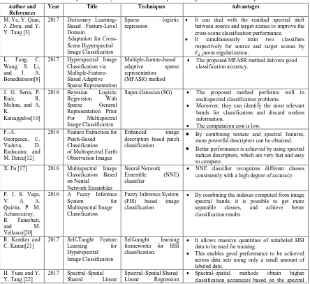
Table I Comparative Analysis of HSI and multispectral image classification techniques Author and

References

Year Title Techniques Advantages

M. Ye, Y. Qian, J. Zhou, and Y. Y. Tang [3]

2017 Dictionary Learning-Based Feature-Level Domain

Adaptation for Cross-Scene Hyperspectral Image Classification

Sparse logistic regression

 It can deal with the residual spectral shift between source and target scenes to improve the cross-scene classification performance.  It simultaneously train two classifiers

respectively for source and target scenes by

ℓ,norm regularization.

L. Fang, C. Wang, S. Li, and J. A. Benediktsson[8]

2017 Hyperspectral Image Classification via Multiple-Feature-Based Adaptive Sparse Representation

Multiple-feature-based adaptive sparse representation (MFASR) method

 The proposed MFASR method delivers good classification accuracy.

J. G. Serra, P.

Ruiz, R.

Molina, and A. K.

Katsaggelos[10]

2016 Bayesian Logistic Regression With Sparse General Representation Prior For Multispectral Image Classification

Super-Gaussian (SG)  The proposed method performs well in multispectral classification problems.

 Moreover, they can identify the most relevant bands for classification and discard useless information.

 The computation cost is low. F.-A.

Georgescu, C. Vaduva, D. Raducanu, and M. Datcu[12]

2016 Feature Extraction for Patch-Based Classification of Multispectral Earth Observation Images

Enhanced image

descriptors based patch classification

 By combining texture and spectral features, more powerful descriptors can be obtained.

 Better performance is achieved by using spectral indices descriptors, which are very fast and easy to compute.

X. Fu [17] 2016 Multispectral Image Classification Based on Neural

Network Ensembles

Neural Network

Ensemble (NNE)

classifier

 NNE classifier recognizes different classes consistently with a high degree of accuracy.

P. J. S. Vega,

V. A. A.

Quirita, P. M. Achanccaray, R. Tanscheit,

and M.

Vellasco[20]

2016 A Fuzzy Inference

System for

Multispectral Image Classification

Fuzzy Inference System (FIS) based image classification

 By combining the indexes computed from image spectral bands, it is possible to get more separable classes, and achieve better classification results.

R. Kemker and C. Kanan[21]

2017 Self-Taught Feature

Learning for

Hyperspectral Image Classification

Self-taught learning frameworks for HSI classification.

 It allows massive quantities of unlabeled HSI data to be used for training.

 This enables good performance to be achieved across data sets using only a small amount of labeled data.

H. Yuan and Y. Y. Tang [22]

2017 Spectral–Spatial Shared Linear

Spectral–Spatial Shared Linear Regression

(8)

ISSN(Online): 2320-9801

ISSN (Print): 2320-9798

I

nternational

J

ournal of

I

nnovative

R

esearch in

C

omputer

and

C

ommunication

E

ngineering

Regression for Hyperspectral Image Classification

method (SSSLR) information.

 The shared structure learning model can further help to learn a more discriminative projection for classification.

S. Jia, B. Deng, J. Zhu, X. Jia, and Q. Li [23]

2017 Superpixel-Based Multitask Learning Framework

for Hyperspectral Image Classification

Gabor Superpixelbased spatial–spectral SchroedingerEigenmaps (S4_{E) and SVM-based}

multitask learning (GS4_E-MTL

SVM)

 The proposed method can achieve more distinct features, which greatly increase the computational efficiency of the dimensionality reduction procedure.

 Minimum computational time.

W. Zhao, L. Jiao, W. Ma, J. Zhao, J. Zhao, H. Liu [26]

2017 Superpixel-Based Multiple Local CNN for

Panchromatic and Multispectral Image Classification

Superpixel-based

multiple local

convolution neural network (SML-CNN) model

 The accuracy rate is improved.

IV.CONCLUSION

Satellite image classification is an exciting area of research due to the availability of large amount of remotely sensed data and requirement in multiple applications. The main function of the classification technique is to generate land cover maps from the remote sensed data. The success of the image classification approach depends on many factors such as availability of high-quality image and design of a proper classification procedure. This survey provided a comparative analysis between different types of HSI and multispectral image classification techniques and working knowledge about these classification methods.

REFERENCES

[1] T. Sarath, G. Nagalakshmi, and S. Jyothi, "A study on hyperspectral remote sensing classifications," in International Conference on

Information and Communication Technologies (ICICT), 2014, pp. 5-8.

[2] M. Govender, K. Chetty, V. Naiken, and H. Bulcock, "A comparison of satellite hyperspectral and multispectral remote sensing imagery for improved classification and mapping of vegetation," Water SA, vol. 34, pp. 147-154, 2008.

[3] M. Ye, Y. Qian, J. Zhou, and Y. Y. Tang, "Dictionary Learning-Based Feature-Level Domain Adaptation for Cross-Scene Hyperspectral Image Classification," IEEE Transactions on Geoscience and Remote Sensing, 2017.

[4] Y. Qian, M. Ye, and J. Zhou, "Hyperspectral image classification based on structured sparse logistic regression and three-dimensional wavelet texture features," IEEE Transactions on Geoscience and Remote Sensing, vol. 51, pp. 2276-2291, 2013.

[5] A. Beck and M. Teboulle, "A fast iterative shrinkage-thresholding algorithm for linear inverse problems," SIAM journal on imaging sciences, vol. 2, pp. 183-202, 2009.

[6] A. Singh, M. Srivatsa, and L. Liu, "Search-as-a-service: Outsourced search over outsourced storage," ACM Transactions on the Web (TWEB), vol. 3, p. 13, 2009.

[7] X. Chen, Q. Lin, S. Kim, J. G. Carbonell, and E. P. Xing, "Smoothing proximal gradient method for general structured sparse regression,"

The Annals of Applied Statistics, pp. 719-752, 2012.

[8] L. Fang, C. Wang, S. Li, and J. A. Benediktsson, "Hyperspectral Image Classification via Multiple-Feature-Based Adaptive Sparse Representation," IEEE Transactions on Instrumentation and Measurement, 2017.

[9] L. Fang, S. Li, X. Kang, and J. A. Benediktsson, "Spectral–spatial hyperspectral image classification via multiscale adaptive sparse representation," IEEE Transactions on Geoscience and Remote Sensing, vol. 52, pp. 7738-7749, 2014.

[10] J. G. Serra, P. Ruiz, R. Molina, and A. K. Katsaggelos, "Bayesian logistic regression with sparse general representation prior for multispectral image classification," in IEEE International Conference on Image Processing (ICIP), 2016, pp. 1893-1897.

[11] J. G. Daugman, "Complete discrete 2-D Gabor transforms by neural networks for image analysis and compression," IEEE Transactions

on Acoustics, Speech, and Signal Processing, vol. 36, pp. 1169-1179, 1988.

[12] F.-A. Georgescu, C. Vaduva, D. Raducanu, and M. Datcu, "Feature extraction for patch-based classification of multispectral earth observation images," IEEE Geoscience and Remote Sensing Letters, vol. 13, pp. 865-869, 2016.

[13] B. S. Manjunath, J.-R. Ohm, V. V. Vasudevan, and A. Yamada, "Color and texture descriptors," IEEE Transactions on circuits and

systems for video technology, vol. 11, pp. 703-715, 2001.

[14] E. Tuncel, P. Koulgi, and K. Rose, "Rate-distortion approach to databases: Storage and content-based retrieval," IEEE Transactions on

Information Theory, vol. 50, pp. 953-967, 2004.

[15] G. Marchisio, F. Pacifici, and C. Padwick, "On the relative predictive value of the new spectral bands in the WorldWiew-2 sensor," in

Geoscience and Remote Sensing Symposium (IGARSS), 2010 IEEE International, 2010, pp. 2723-2726.

[16] S. Cui, G. Schwarz, and M. Datcu, "Remote sensing image classification: No features, no clustering," IEEE Journal of Selected Topics in

Applied Earth Observations and Remote Sensing, vol. 8, pp. 5158-5170, 2015.

(9)

ISSN(Online): 2320-9801

ISSN (Print): 2320-9798

I

nternational

J

ournal of

I

nnovative

R

esearch in

C

omputer

and

C

ommunication

E

ngineering

[18] Y. Liu and X. Yao, "Ensemble learning via negative correlation," Neural Networks, vol. 12, pp. 1399-1404, 1999.

[19] H. Chen and X. Yao, "Regularized negative correlation learning for neural network ensembles," IEEE Transactions on Neural Networks,

vol. 20, pp. 1962-1979, 2009.

[20] P. J. S. Vega, V. A. A. Quirita, P. M. Achanccaray, R. Tanscheit, and M. Vellasco, "A fuzzy inference system for multispectral image classification," in ANDESCON, 2016 IEEE, 2016, pp. 1-4.

[21] R. Kemker and C. Kanan, "Self-taught feature learning for hyperspectral image classification," IEEE Transactions on Geoscience and

Remote Sensing, vol. 55, pp. 2693-2705, 2017.

[22] H. Yuan and Y. Y. Tang, "Spectral–spatial shared linear regression for hyperspectral image classification," IEEE transactions on cybernetics, vol. 47, pp. 934-945, 2017.

[23] S. Jia, B. Deng, J. Zhu, X. Jia, and Q. Li, "Superpixel-Based Multitask Learning Framework for Hyperspectral Image Classification,"

IEEE Transactions on Geoscience and Remote Sensing, vol. 55, pp. 2575-2588, 2017.

[24] V. Nair and G. E. Hinton, "Rectified linear units improve restricted boltzmann machines," in Proceedings of the 27th international

conference on machine learning (ICML-10), 2010, pp. 807-814.

[25] A. Krizhevsky, I. Sutskever, and G. E. Hinton, "Imagenet classification with deep convolutional neural networks," in Advances in neural

information processing systems, 2012, pp. 1097-1105.

[26] W. Zhao, L. Jiao, W. Ma, J. Zhao, J. Zhao, H. Liu, et al., "Superpixel-Based Multiple Local CNN for Panchromatic and Multispectral Image Classification," IEEE Transactions on Geoscience and Remote Sensing, 2017.

BIOGRAPHY