Implementation of Back Propagation Neural Network with PCA for Face Recognition

© 2019.Md. Manik Ahmed, A F M Zainul Abadin, Md. Anwar Hossain & Md. Imran Hossain. This is a research/review paper, distributed under the terms of the Creative Commons Attribution-Noncommercial 3.0 Unported License http://creativecommons.org/licenses/by-nc/3.0/), permitting all non-commercial use, distribution, and reproduction in any medium, provided the original work is properly cited.

Global Journal of Computer Science and Technology: G

Interdisciplinary

Volume 19 Issue 3 Version 1.0 Year 2019

Type: Double Blind Peer Reviewed International Research Journal

Publisher: Global Journals

Online ISSN:

0975-4172

& Print ISSN:

0975-4350

Implementation of Back Propagation Neural Network with PCA for

Face Recognition

By Md. Manik Ahmed, A F M Zainul Abadin, Md. Anwar Hossain & Md. Imran Hossain

Rabindra Maitree University

Abstract-

Face recognition is truly one of the demanding fields of biometric image processing system.

Within this paper, we have implemented Back Propagation Neural Network for face recognition using

MATLAB, where feature extraction and face identification system completely depend on Principal

Component Analysis (PCA). Face images are multidimensional and variable data. Hence we cannot

directly apply Back Propagation Neural Network to classify face without extracting the core area of face.

So, the dimensionality of face image is reduced by the Principal Component Analysis algorithm then we

have to explore unique feature for all stored database images called eigenfaces of eigenvectors. These

unique features or eigenvectors are given as parallel input to the Back Propagation Neural Network

(BPNN) for recognition of given test images. Here test image is taken from the integrated webcam which

is applied to the BPNN trained network. The maximum output of the tested network gives the index of

recognized face image. BPNN employing PCA is more robust and reliable than PCA based face

recognition system.

Keywords:

face detection, face recognition, principal component analysis (PCA), eigenfaces, back

propagation neural network (BPNN).

GJCST-G Classification:

I.2.6

ImplementationofBackPropagationNeuralNetworkwithPCAforFaceRecognition

(

)

G

Global Journal of Computer Science and Technology Volume XIX Issue III Version I

Year

2 019

Implementation of Back Propagation Neural

Network with PCA for Face Recognition

Md. Manik Ahmed

, A F M Zainul Abadin

, Md. Anwar Hossain

& Md. Imran Hossain

Abstract- Face recognition is truly one of the demanding fields of biometric image processing system. Within this paper, we have implemented Back Propagation Neural Network for face recognition using MATLAB, where feature extraction and face identification system completely depend on Principal Component Analysis (PCA). Face images are multidimensional and variable data. Hence we cannot directly apply Back Propagation Neural Network to classify face without extracting the core area of face. So, the dimensionality of face image is reduced by the Principal Component Analysis algorithm then we have to explore unique feature for all stored database images called eigenfaces of eigenvectors. These unique features or eigenvectors are given as parallel input to the Back Propagation Neural Network (BPNN) for recognition of given test images. Here test image is taken from the integrated webcam which is applied to the BPNN trained network. The maximum output of the tested network gives the index of recognized face image. BPNN employing PCA is more robust and reliable than PCA based face recognition system.

Keywords: face detection, face recognition, principal

component analysis (PCA), eigenfaces, back propagation neural network (BPNN).

I.

I

he human face represents a significant role in our social conversation, contain people’s identity. In the past several years, Face recognition has been regarded as an important research subject in the area of Digital image processing (DIP) and Computer Vision mainly because of over growing security demand and both law or non-law enforcement.

The human face plays an important role in our social interaction; also contain people’s identity and emotions among them. The human faces represent complex, multidimensional, meaningful visual stimulant. Developing a computational model for face recognition is difficult [1].

The primary approach for face recognition is face detection. It is easy and efficient for highly correlated biological neuron in the human brain. Even a small child can perfectly authenticate a human but it is difficult task for a computer. Here we present a

Author α: Department of Information and Communication Engineering

(ICE), Rabindra Maitree University, Kushtia, Bangladesh. e-mail: [email protected]

Authors σ ρ Ѡ: Department of Information & Communication

Engineering (ICE), Pabna University of Science and Technology (PUST), Pabna, Bangladesh. e-mails: [email protected],

[email protected], [email protected]

mathematical model and computational model for face recognition that act as like as a human brain.

Due to the variational behavior of human face image, we need to extract unique feature. There are numerous strategies applied for this purpose. In this paper we have used principal component analysis algorithm to extract feature called Eigenfaces by modifying the image into one column and building a single matrix i.e. we must find the axis in which covariance matrix is diagonal or we determine a direction or a new axis where the data variation is the greatest. Then we find another direction where the remaining data variation is the greatest. But this two axes or direction is orthogonal from one another. The objective of PCA is usually to decrease the dimensionality of the image while retaining as a lot of information as possible in the original image. Using PCA we have calculated eigenface then all database face image projected on this eigenface space and we got a new face descriptor or feature vectors or weights matrix.

The eigenfaces or the principal Components of the faces are eigenvectors of the matrix and it is the eigenvectors. This combination of eigenvectors parallely given to the Back Propagation Neural Network input neuron. Training process in BPNN happens by back propagate the error and adjusting weights of each and every link. After training and testing is done by test image applied to the fully trained network. The maximum value of the tested network gives the recognized image index.

Face image is actually a biometrics physical feature which is used to verify the individuality of people. The main components involved in the face image space include mouth, nose, and eyes. Among various biometrics characteristics face is the most physical entity for identify among people [2]. Face identification can be done significantly by capturing devices using digital cameras or webcam.

II.

L

R

This section quickly discusses the pattern recognition process and after that highlights some of the current research in the area of autonomous face recognition. Traditionally, pattern recognition is split up three areas: (1) segmentation, (2) feature extraction, and (3) classification [3]. Segmentation is the first step; it is finding regions of possible signals. The second stage is feature extraction and in this task we search for the most

T

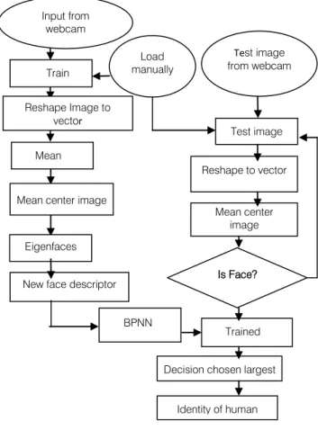
Fig.1: Proposed Block diagram

b) Eigenface Calculation and Feature Extraction by PCA

An image is a two dimensional function I(x, y); so we consider the 2D case where we have an input image and compare this with the database to achieve the recognition goal. We also consider that the images are all of the same resolution. Each pixel can be regarded as a variable thus we have a very large dimensional problem which can be simplified by PCA. In image recognition an input image or test image with n×n pixels can be considered as a point in_n2_{dimensional space called the image space. The}

coordinates of this point describes the values of each and every pixel of the image and form a column vector. This vector is formed by concatenating each column of 306×251resolution image; it will dimension 76806 so form of the vector is 76806 rows and 1 column.

After face database D is set then all images in the face database reshape to vector and forming a matrix which indicate the image matrix where number of column equal to the number of face image in database or training set. Here we have M images each with n2

pixels. We can write our entire data set as an n2_{×M data}

matrix D. Each column of D represents one image of our data set. Then concatenate column images form into one matrix. D = {Γ1,Γ2,Γ3, … … … ,ΓM} (1) Input from webcam Train Load manually Reshape Image to vector Mean

Mean center image

Eigenfaces New face descriptor

BPNN

Trained Decision chosen largest

Identity of human Mean center image Reshape to vector Test image Is Face? Test image from webcam

(

)

G

Global Journal of Computer Science and Technology Volume XIX Issue III Version I

Implementation of Back Propagation Neural Network with PCA for Face Recognition important or significant features of the regions passed

by the segmentor which can be used in the last step, classification. Classification analyzes the extracted features to those of previously identified objects and identifies the object as one of the previously identified classes.

recognition [4]. The first approach is local based, this approach based on some number of distinct feature on the face are recorded manually or through feature extraction modules. The features used in local based face recognition are the nose position, nostril position, eye brows positions, eyes position, mouth position and chin position etc. This data is then processes usually either through the neural network or some statistical method is used for the recognition process. Yullie and Cohen used deformable templates in contour extraction of face images [5]. Another approach is holistic based, in this approach; the whole face is used for face recognition instead of taking only some local data. This may include a simple template matching or more sophisticated method such as PCA based method to extract the principle components for that huge set of data and reduced it into a smaller group of data. Matthew Turk and Alex Pentland, from the Massachusetts Institute of Technology Media Lab, have implemented this system for face recognition that also makes use of the Karhunen-Lobve Transform [1].

III.

M

M

Our proposed technique based upon Principal Component analysis and Back Propagation Neural Network multilayer Classifier. Our proposed block diagram of face recognition procedure is as shown Figure 1.

a) Preprocessing and Face Database

The preprocessing of the images are Image size normalization, Histogram equalization, Median filtering and conversion RGB image to gray scale image. This module automatically takes same dimension image and perform preprocessing step in order to improve face recognition performance. The first criteria for face recognition is create a face database which contains all face images for training. There are two step to create face database: first, one is image taken from the live webcam and stored it to face database. Another one is image taken from a folder or disk storage or another external memory. Suppose total number of face image in this database is ‘M’. Another important thing we should take all images in same dimension. In our system we take all image in the dimension of 306_×251.

Then we calculated mean image of whole face image in database using the reshaped face matrix. We accomplished this by finding a mean image Ψ by averaging the columns of D matrix.

Ψ=_M1∑Mn=1 (2) Γn

The calculation process is,

Mean image =∑Column of reshaped face matrix_{Total number of column}

We need to adjust the images by subtract the computed average image from each image in the database. Consequently, the origin is moved to the mean of the data and this creates the mean centered data matrix.

Φi=Γi− Ψ (3)

So the Adjusted image matrix is,

A=[Φ1,Φ2,Φ3,Φ4………….ΦM] (4)

These Adjusted images determine how each of the images in database differs from the average face.

We need calculate the M×M matrix to find its eigenvalues and eigenvectors and we selected the k eigenvectors with the highest related eigenvalues. As a property to the eigenvector, each of them has an eigenvalue associated with it. More valuable eigenvectors with greater eigenvalues supply more information on the face variation than those with smaller eigenvalues. Here images are matrix represented so we must need to compute covariance matrix of image matrix for determine the eigenvector. It is extremely simple to compute the covariance matrix from the mean centered data matrix. So, the equation of covariance matrix is,

C =_M1∑Mn=1ΦnΦnT ₍₅₎

= AAT

But Here a little problem in the output of covariance matrix. Where matrix dimension n2_{× n}2 _{that is too big,}

even it exceeds the total quantity of face images in the database and also break the condition eigenface ≤ M. Then the correct calculation of eigen vector Vi of ATA

AT_AV

i=λi (6) ∗Ui

Eigenvectors with smaller eigenvalues lead tiny information in the data representation. Now compute the M best eigenvectors from covariance matrix and keep exactly the K eigenvectors equivalent to the K largest eigenvalues.To calculate the eigenfaces, the normalized or mean centered face multiplied with the highest eigenvector. These vectors describe the linear combinations of the M training set of stored face images which is called eigenfaces Ui.

Ui=∑Mk=1VkΦ (7) k

Once the eigenfaces are taken from the covariance matrix of a collection of faces, every single face is projected onto the eigenface space and represented with a linear combination of the eigenfaces or provide a new descriptor related to a point under the high dimensional space with the eigenfaces as axes. A new face is turned into its eigenface components. Primary we compare our input image with our mean image and multiply their difference with each eigenvector. Every single value would represent a weight and would be saved on a vector Ω.

ωk = UkT(Γ − Ψ) (8)

Where, k = 1……..M. This represents a set of point which determined by image multiplications and summations operations executed at approximately frame rate on current image processing hardware. The weights form a feature vector calculated from the above (8) where each image project on the each of the eigenfaces. So, the new face descriptor is,

ΩT =�ω1,ω2,ω3… … … .ωM� (9)

That describes the best contribution of every eigenfaces in addressing the input face image. The vector are able to be used in a conventional pattern recognition algorithm to find out what of a number of predetermined face class if any best describes the face. The face class can be calculated by averaging the weight vectors for the images of a single person face.

c) Face Detection

The image of a face when projected into the face space does not radically change, while non-face image projection is quite different. Basic idea is always to detect the existence of a face in a scene by calculating the distance from face space. If distance is low then it is a face.

For an unknown image_Γ, compute the mean centered image

Φ=Γ − Ψ (10)

Now every face inside the training database set (minus the mean), Φican be described as a linear

combination of these Eigenvectors or eigenfaces. Φi=∑ki=1(ωiUi) (11)

These weights may be computed as,

ωi= UiTΦ (12) i

Then compute the Euclidean distance ed of

unknown image from face Space.

ed =‖Φ − Φi‖ (13)

If ed is less than specific threshold thenΓ is a face

d) Face Reconstruction

Each Normalized face _Φiin A can be represented as a linear combination of the best k

(

)

G

Global Journal of Computer Science and Technology Volume XIX Issue III Version I

Year

eigenvectors. So face reconstruction is very easy process by using eigenvectors. First we need to calculate weighted sum of all eigenfaces which is the reconstructed original image is equivalent to sum of all eigenfaces with every eigenface contain a certain weight. This weight describes to what amount of specific feature is present in the original image. If one face uses all the eigenfaces which is obtained from original face images it is possible to rebuild the main images from the eigenfaces exactly. Then this reconstructed image is definitely an approximation of the original image.

Now every face inside the training database set (minus the mean), Φican be described as a linear

combination of these Eigenvectors or eigenfaces.

Φi =∑ki=1(ωiUi) (14)

These weights may be computed as,

ωi= UiTΦ (15) i

Where i = 1, 2... M. This means we have to calculate such a vector corresponding to every image in the training set and store them as template. InΦi, where

i is a number which indicates that which person face we want to reconstruct

e) Back Propagation Neural Network

In 1986, a group of scientists led by Rumelhart. J.L. McClelland and D.E. put forward a type of error back-propagation algorithm for training multilayer feedforward neural network, which is one of the widely used networks [6]. The generalized delta rule [7 8] also referred to as backpropagation algorithm criteria is explained here briefly for feed forward neural network (NN). The NN explained here consist of 3 layers. This 3 layer are input, hidden, and output Layers. During the training phase, the training data is fed parallel to the input layer. The data are propagated to the hidden layer and then to the output layer. This process is known as the forward move of the BPNN algorithm. The error involving in actual output values and target output values is calculated and propagated back toward hidden layer to input layer. This process is known as the backward move of the BPNN algorithm.

f) BPNN Algorithm

The back propagation algorithm performs like this,

Step 1: First apply the inputs to the network to get the network output simply. Now remember this initial output could be anything, as the initial weights were random numbers between -0.3 to 0.3.

Step 2: For every node of output, simply calculate the error. The error is what you want - What you actually get. In other words,

δK=ΟK(1−ΟK)(ΟK−T) (16)

The ΟK(1−ΟK) term is essential in the equation

due to the Sigmoid Function, if we were only using a threshold neuron it would just be(ΟK−T).

Step 3: Then calculate the Errors for theneurons of hidden layer.

δJ=ΟK(1−ΟK)∑kεKδKWJK (17)

Where,WJK is the weight between layers J to layer K.

Step 4: For every Iteration, Update the weights and biases are as follows

Updated weight, ∆W =−ηδlΟl−1

Updated Bias,∆θ=−ηδl

Where negative signs determine back propagate the errors and the constant ηis the learning rate is put in to speed up or slow down the learning if required.

Then apply,

W +∆W→W

θ+∆θ → θ

Step 5: Having acquired the Error for that hidden layer neurons now proceed as in step 4 to change the hidden layer weights. By reiterating this method, we can train a network of any number of layers. Back Propagation Neural network is broadly used pattern classification algorithm which reverse propagates the error and adjusts the weights to near the target output.

g) Face Recognition Using BPNN

After feature extraction we have to create neural network. We created neural network one for each person in the database. Then extracted feature vectors are fed as inputs to train each person's networks.

In training, the faces feature vectors that belong to same person are used as positive examples for the person’s network i.e. network gives 1 as output, and negative examples for the others network i.e. Network gives 0 as output which the target value were. The algorithm used to train the network is the back propagation Algorithm. The basic idea with the back propagation algorithm is to use gradient descent to update the weights so as to minimize the mean squared error between the network output values and the target output values. The update procedures are derived by taking the partial derivative from the error function with regards to the weights to find out each weight's contribution to the error. Then every weight is modified using gradient descent based on its participation to the error. The activation or transfer function use in Back Propagation neural network is sigmoid function which maps the output 0 to 1. With the effective operation of the back propagation network it is necessary for the appropriate selection of the parameters used for training. We have used initialize weights between -0.3 to 0.3 and here number of output neuron equal to number of input neuron because each network equal to the one person. In this training process we keep the learning rate 0.05 and hidden neuron 50.Also we have an option to change the hidden neuron for every execution. Here

(

)

G

Global Journal of Computer Science and Technology Volume XIX Issue III Version I

too few hidden units will prevent the network from being able to learn the required function, because it will have too few degrees of freedom. Too many hidden units may cause the network have a tendency to over fit the training data thus reducing generalization accuracy. Though learning rate is low but it gives the better accuracy than highest one. Additionally a small learning rate is used to avoid main disruption of the direction of learning when extremely unusual pair of training patterns is presented. When neural network met the stopping condition then it stops and gives the train output.

In testing, a new image is taken for recognition from face database or live webcam. We reshape this image to vector and calculated normalized image. This normalized face images are compared with the reconstructed face image. If Euclidian distance between two images is minimum or less than predefined threshold, then it is face otherwise this is not face. If this is face, then we are ready for testing the human face for recognition.

Before testing we need to extract feature of this unknown human face. Its feature vectors are determined from the eigenfaces identified before, and this image receives its new descriptors. These new descriptors are inputted to each network and also the networks are simulated using these descriptors. The network outputs are compared. If the maximum output exceeds the predefined threshold level, then this new face is decided to belong to person with this maximum output.

IV.

E

R

D

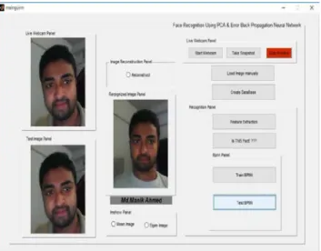
The Graphical User Interface was constructed using MATLAB GUIDE or Graphical User Interface Design Environment. Using the layout tools provided by GUIDE, we have designed the following graphical user interface figure (mainguinn.fig) for the face recognition user application.

Fig.2: Graphical interface of proposed system with test image from webcam

Training and Testing Images: Training images are taken by the webcam and we have created a database which contains 25 images under different lighting condition. Also we have an option for load image manually to create database. Here some images of our database,

Fig.3:Training images of image database taking from webcam

Also our system checks the provide test image face or not face which is the part of face detection and give a confirmation message after face recognition.

Fig.7:Face detection confirmation message

Fig.8:Face recognition confirmation message

(

)

G

Global Journal of Computer Science and Technology Volume XIX Issue III Version I

Year

2 019

Fig. 4:Test image Fig. 5: Mean image Fig. 6: Recognized image

Fig.9:Graphical interface after face recognition

Face Reconstruction: The reconstructed image is undoubtedly an approximation of the original image.

Accuracy Calculation: We have tested on 25 images which are taken from webcam and database. Accuracy can be calculated using the following formula,

Accuracy=_{Total number}Correctly_ofimagetested_tobetasted × 100 Face detection Accuracy=20₂₅× 100 = 80%

Face Recognition Accuracy when test image taken from webcam

=23_{25 × 100 = 92%}

Face Recognition Accuracy when test image taken from Database

=25₂₅× 100 = 100%

V.

C

In this paper, Eigen face represented features vectors are used for face recognition. The features are obtained from the face image to shows unique identity of human face utilized as inputs to the neural network for classification. Eigenfaces are the most significant feature and reduce the size of input of neural network. This system performs human face recognition at a very

high degree of accuracy. We encountered several problems in these experiments due to the lighting variation. However, we can overcome this issue by normalize the illumination. This is a biometric system and the work can be surely used in biometric applications like access control and verification systems.

R

R

R

1. M.A.Turk and A.P.Petland, “Eigenfaces for Recognition,” Journal of Cognitive Neuroscience, vol. 3, pp.71-86, 1991.

2. Ravi Prakash, “An Efficient Back Propagation Neural Network Based Face Recognition System Using Haar Wavelet Transform and PCA,” international Journal of research review in engineering science and technology, Vol.2, ISSUE.2, June 2013.

3. Tou, Julius C. and Rafael C. Gonzalez., “Pattern Recognition Principles,” Addison Wesley Publishing, 1974.

4. Gul, A.B., “Holistic face recognition by dimension reduction,” The graduate school of natural and applied science of the middle east technical university, p. 121, 2003.

5. Yuille, A.L., Cohen, D.S., and Hallinan, P.W.," Feature extraction from faces using deformable templates", Proc. of CVPR, 1989.

6. Yong He, “Application Research of BP neural network in face recognition,” International Conference on Information Sciences, Machinery, Materials and Energy, 2015.

7. D. E. Rumelhart, G. E. Hinton, and R. J. Williams. Leaning Internal Representaions by Ewvr Propagation in Rumelhart, D. E. and McClelland, J. L., Pamllel Distributed Processing: Explorations in the Microstructure of Cognition. MIT Press, Cambridge Massachusette, 1986.

8. Jamshid Nazari, Okan K. Ersoy, “Implementation of back-propagation neural networks with MatLab,” Jan 1992.

Fig.10:Original image Fig.11: Reconstructed image

(

)

G

Global Journal of Computer Science and Technology Volume XIX Issue III Version I