Departamento de Teor´ıa de la Se˜nal y Comunicaciones
DOCTORAL THESIS
BAYESIAN NONPARAMETRIC MODELS
FOR DATA EXPLORATION
Author: M ´
ELANIE NATIVIDAD FERN ´
ANDEZ PRADIER
Supervised by: FERNANDO P ´
EREZ CRUZ
Autor: M´elanie Natividad Fern´andez Pradier
Director: Fernando P´erez Cruz
Fecha: September 15th, 2017
Tribunal
Presidente: Joaqu´ın M´ıguez Arenas
Vocal: C´edric Archambeau
Secretario: Daniel Hern´andez Lobato
“自分を信じる力、それが運命を変える力となる。”
A mis padres, Fernando y Marie-Th´er`ese, por su apoyo incondicional. A Nii-san, por mostrarme el camino y forjarme el car´acter. A Javier, por estar siempre a mi lado.
When I was little, I remember trying to na¨ıvely decipher my elder brother’s notebook, which was full of integrals, and ending up crying because I was not able to understand such mysteries. Back then, I felt an immense wall raising in front of me, which I could finally demolish a few years later. Since then, I have vitally wandered, challenge after challenge, always seeking to confront the most fulfilling trials.1. Pick and shovel on my shoulder, I decided to leave the industry career path and start my new academic quest. Fall, winter, spring, and next was summer. The cherry trees blossomed late May, and this thesis needed to come to an end: I am ready to tear down this new facade.
But now more than ever, I am bitterly aware of the immensity of ignorance: the many things I do not know and that I will probably never get to know. Also now more than ever, I am able to comprehend the beauty of life and knowledge, and the exceptional talent of people around me, which have been an infinite (nonparametric) source of inspiration during these years. This thesis is not a masterpiece, but I have made endless sacrifices in the learning path, and put an immeasurable effort in its accomplishment, which is the best way I can now truly thank all those people who believed in me and stood by me all along.
To begin with, I would like to express my deep gratitude to my supervisor Fernando P´erez-Cruz for never losing faith in me, always granting me the freedom to pursue my own research direction, and teaching me the Yamamoto’s challenging way of “working with delight”. The signal theory and communications group at Universidad Carlos III de Madrid (UC3M) has been a fantastic learning environment where I have had the privilege to meet remarkable people. In particular, I would like to thank my academic siblings: Francisco J. R. Ruiz, for nurturing my passion for science, games and desserts; Isabel Valera, for her warm hugs and tenacity within research; Pablo M. Olmos, for his valuable mentorship in science, basketball and arcade games. Thanks to Victor Elvira for a shared complicity and feverish passion for multidisciplinary subjects; thanks to Pablo G. Moreno
1
towards science and constant good-nature. I would also like to thank Antonio Art´es for adopting me in the GTS family, and for our open discussions about different ways of living and types of wines. Also thanks to the new generation, Pablo Bonilla and Pablo Moreno, for your sparking enthusiasm and steady willingness to make your utmost. Many thanks to Grace Villacr´es, Francisco Hernando, David Ram´ırez, Gonzalo R´ıos, and Alberto Valera for sharing an uncountable number of coffees and good chats together. Thank you to Paloma Vaquero for her sunny friendship and unshakable smile no matter what the difficulties might be. I would also like to thank Harold Molina-Bulla and Ana Hernando for their constant help along these years, as well as Marcelino L´azaro, for his guidance in the art of teaching.
Outside the UC3M, I feel very thankful to the GAPS research group within the signal processing department at the Universidad Polit´ecnica de Madrid (UPM), which accepted me wholeheartedly in their scientific discussions with regularity. Thank you to Santiago Zazo for all the philosophical wanderings while running moderately across fields. Truly thanks to Sergio Valcarcel, whose positiv-ity and kindness are beyond any limit; Marta Mart´ınez, for her valuable friendship and contagious love for music; Pavle Belanovic, for showing me an endless enthousiasm for scientific and personal undertaking.
Special thanks to the European Marie Curie Initial Training Network sponsorship and colleagues within the network, with special mention to Felipe Llinarez, Dean Bodenham, Laetitia Papaxanthos, Crist´obal Esteban, Yi Zhong, Ramouna Fouladi, and Yunlong Jiao. I feel indebted for your friend-ship and enriching discussions via Skype, summer schools, research stays and conferences. I am also extremely grateful to my external collaborators: Francesca Milletti and Oscar Puig from Roche Di-agnostics in New York; Viktor Stojkoski, Zoran Utkovski and Ljupco Kocarev from the Macedonian Institute of Science and Arts; Stephanie Hyland, Stefan Stark, Julia E. Vogt and Gunnar R¨atsch from the Memorial Sloan-Kettering Cancer Center in New York; Kridsadakorn Chaichoompu, Fentaw Abegaz, and Kristel Van Steen from the University of Li`ege.
Naoki Kamimaeda and Masanori Miyahara for their incalculable guidance and support during my research internship in Japan, and towards all members of the former IAV department for receiving me with open arms in their group during a period of time that left a profound imprint on my spirit, strengthening my character and perseverance skills.
On the personal side, I would like to thank my dear friend Pedro A. De Mattos, whose antithetical vision of the world has enriched me enormously and led me to valuable compromises within soci-ety; also thanks to Luis Jou for displaying a regular, undisturbed passion for life and work. Thank you to Constanza Blanco for trying to make from the world a better place together. I am grateful to all the friends I met in Germany, specially in the kitchen from Allmandring 20C in Stuttgart (Tim-otheus, Tomoko, Simon, Haitham, Jonas, Diego, Chisato, among others),as well as my childhood friends who always believed in me (Sara, Raquel, Clara, Nuria and Alba). I cannot forget mention-ing Guillermo, Berta, Andr´es, and Elena, for the intense debates and wonderful trips together.
The achievement of this doctoral thesis would have never been possible without the unwavering support of my family and beloved ones. Thank you to my parents and brother, I owe you more than I could possibly express with words. Thanks to Pilar, Clara, and Tanis, for all their affection and understanding during these years. I would also like to thank all the little fur balls (rabbits, cats and dog) which have contributed with their expertise on stress management: Yan, Sid and Leia, Tigre and Nala, Gea, Puchi and Take, Taiko and the little Beibei. Finally, I am truly thankful to Javier Zazo for all the thoughtful discussions about physics, life, the universe, and beyond: you started ariver
of savvy words in the blazing night drift, and have been there for me since then, understanding me,
encouraging me, and suffering me during the whole PhD.
All in all, thanks to all friends, family and colleagues that have been with me at some point in my life and that - I hope - will stay connected. This doctoral thesis is hopefully just the starting door to more exciting research and inspiring encounters in the future. Hopefully, ten years from now when I look into these pages, cracking down the PhD wall might appear as a child’s play.
Making sense out of data is one of the biggest challenges of our time. With the emergence of technologies such as the Internet, sensor networks or deep genome sequencing, a truedata explosion
has been unleashed that affects all fields of science and our everyday life. Recent breakthroughs, such as self-driven cars or champion-level Go player programs, have demonstrated the potential benefits
fromexploitingdata, mostly in well-defined supervised tasks. However, we have barely started to
actuallyexploreand truly understand data.
In fact, data holds valuable information for answering most important questions for humanity: How does aging impact our physical capabilities? What are the underlying mechanisms of cancer? Which factors make countries wealthier than others? Most of these questions cannot be stated as well-defined supervised problems, and might benefit enormously from multidisciplinary research efforts involving easy-to-interpret models and rigorous data exploratory analyses. Efficient data ex-ploration might lead to life-changing scientific discoveries, which can later be turned into a more im-pactful exploitation phase, to put forward more informed policy recommendations, decision-making systems, medical protocols or improved models for highly accurate predictions.
This thesis proposes tailored Bayesian nonparametric (BNP) models to solve specific data ex-ploratory tasks across different scientific areas including sport sciences, cancer research, and eco-nomics. We resort to BNP approaches to facilitate the discovery of unexpected hidden patterns within data. BNP models place a prior distribution over an infinite-dimensional parameter space, which makes them particularly useful in probabilistic models where the number of hidden param-eters is unknown a priori. Under this prior distribution, the posterior distribution of the hidden pa-rameters given the data will assign high probability mass to those configurations that best explain the observations. Hence, inference over the hidden variables can be performed using standard Bayesian inference techniques, therefore avoiding expensive model selection steps.
This thesis is application-focused and highly multidisciplinary. More precisely, we propose an automatic grading system for sportive competitions to compare athletic performance regardless of age, gender and environmental aspects; we develop BNP models to perform genetic association and biomarker discovery in cancer research, either using genetic information and Electronic Health Records or clinical trial data; finally, we present a flexible infinite latent factor model of international trade data to understand the underlying economic structure of countries and their evolution over time.
Uno de los principales desaf´ıos de nuestro tiempo es encontrar sentido dentro de los datos. Con la aparici´on de tecnolog´ıas como Internet, redes de sensores, o m´etodos de secuenciaci´on profunda del genoma, una verdaderaexplosi´on digitalse ha visto desencadenada, afectando todos los campos cient´ıficos, as´ı como nuestra vida diaria. Logros recientes como pueden ser los coches auto-dirigidos o programas que ganan a los seres humanes al milenario juego del Go, han demostrado con creces los posibles beneficios que podemos obtener de laexplotaci´on de datos, mayoritariamente en tareas supervisadas bien definidas. No obstante, apenas hemos empezado con laexploraci´on de datosy su verdadero entendimiento.
En verdad, los datos encierran informaci´on muy valiosa para responder a muchas de las pregun-tas m´as importantes para la humanidad: ¿C´omo afecta el envejecimiento a nuestras aptitudes f´ısicas? ¿Cu´ales son los mecanismos subyacientes del cancer? ¿Qu´e factores explican la riqueza de ciertos pa´ıses frente a otros? Si bien la mayor´ıa de estas preguntas no pueden formularse como proble-mas supervisados bien definidos, ´estas pueden ser abordadas mediante esfuerzos de investigaci´on multidisciplinar que involucren modelos f´aciles de interpretar y an´alisis exploratorios rigurosos. Ex-plorar los datos de manera eficiente abre potencialmente la puerta a un sinn´umero de descubrimientos cient´ıficos en diversas ´areas con impacto real en nuestras vidas, descubrimientos que a su vez pueden llevarnos a una mejor explotaci´on de los datos, resultando en recomendaciones pol´ıticas adecuadas, sistemas precisos de toma de decisi´on, protocolos m´edicos optimizados o modelos con mejores ca-pacidades predictivas.
Esta tesis propone modelos Bayesianos no-param´etricos (BNP) adecuados para la resoluci´on es-pec´ıfica de tareas explorativas de los datos en diversos ´ambitos cient´ıficos incluyendo ciencias del deporte, investigaci´on contra el c´ancer, o econom´ıa. Recurrimos a un planteamiento BNP para fa-cilitar el descubrimiento de patrones ocultos inesperados subyacentes en los datos. Los modelos BNP definen una distribuci´on a priori sobre un espacio de par´ametros de dimensi´on infinita, lo cual los hace especialmente atractivos para enfoques probabil´ısticos donde el n´umero de par´ametros la-tentes es en principio desconocido. Bajo dicha distribuci´on a priori, la distribuci´on a posteriori de los par´ametros ocultos dados los datos asignar´a mayor probabilidad a aquellas configuraciones que mejor explican las observaciones. De esta manera, la inferencia sobre el espacio de variables ocultas puede realizarse mediante t´ecnicas est´andar de inferencia Bayesiana, evitando el proceso de selecci´on de modelos.
List of Acronyms 7
1 Introduction 9
1.1 Motivation . . . 9
1.2 Scientific Aims and Perspective . . . 11
1.3 Contributions . . . 12
1.4 Organization . . . 14
2 Overview of Bayesian Nonparametrics 15 2.1 Introduction . . . 15
2.2 Intuition behind Bayesian Nonparametric Models . . . 18
2.3 Random Measures . . . 21
2.3.1 Dirichlet Process . . . 23
2.3.2 Beta Process . . . 27
2.4 Inference Methods . . . 30
2.5 Summary . . . 31
3 Atom-Dependent Dirichlet Process for Marathon Modeling 33 3.1 Introduction . . . 34
3.2 Dependent Dirichlet Processes . . . 34
3.3 Our Approach . . . 36
3.3.1 Atom-Dependent Dirichlet Process Mixture Model . . . 36
3.3.2 Further Model Extensions . . . 38
3.4 Results . . . 40
3.4.1 Density Estimation . . . 41
3.6.3 Simulations . . . 64
3.7 Summary . . . 66
4 Case-Control Indian Buffet Process for Analysis of Clinical Trials 67 4.1 Introduction . . . 68
4.2 General Latent Feature Model . . . 69
4.3 Our Approach . . . 71
4.3.1 Modeling . . . 72
4.3.2 Inference . . . 73
4.3.3 Statistical Methodology . . . 74
4.4 Results . . . 77
4.4.1 Antibody Treatment for Hepatocellular Carcinoma . . . 78
4.4.2 Identified Subpopulations . . . 78
4.4.3 Discovered Biomarkers . . . 80
4.4.4 Discussion . . . 83
4.5 Summary . . . 83
4.A Appendix: General Latent Feature Modeling Toolbox . . . 85
4.B Appendix: Details on the phase II Clinical Trial for Codrituzumab . . . 94
5 Hierarchical Indian Buffet Process for Discovery of Genetic Associations 99 5.1 Introduction . . . 100
5.2 Genetic Association Studies . . . 101
5.2.1 Standard Approach: Case-Control Setup . . . 103
5.2.2 Confounder Correcting Approach: Linear Mixed Model . . . 103
5.3 Our Approach . . . 104
5.3.1 Bernoulli Process Poisson Factor Analysis . . . 104
5.4 Results . . . 106
5.4.1 Database Description . . . 106
5.4.2 Experimental Setup . . . 107
5.4.3 Identification of Clinico-Genetic Associations . . . 107
5.5 Summary . . . 112
5.A Appendix: Complete List of Associations . . . 115
6 Flexible Indian Buffet Process Priors for Understanding International Trade 121 6.1 Introduction . . . 122
6.2 Flexible IBP Extensions . . . 124
6.2.1 Three-Parameter Indian Buffet Process . . . 124
6.2.2 Restricted Indian Buffet Process . . . 124
6.3 Static Scenario . . . 125
6.3.1 Three-Parameter Restricted Bernoulli Process Poisson Factor Analysis . . . . 125
6.3.2 Inference . . . 127
6.4 Time-varying Scenario . . . 128
6.4.1 Dynamic Bernoulli Process Poisson Factor Analysis . . . 128
6.4.2 Inference . . . 129 6.5 Results . . . 130 6.5.1 Static Scenario . . . 131 6.5.2 Time-varying Scenario . . . 137 6.6 Summary . . . 143 7 Conclusions 145 7.1 Summary . . . 145 7.2 Future Work . . . 147 7.3 Discussion . . . 151
8 Inference Details for Poisson Factor Analysis Models and Extensions 155 8.1 Poisson Factor Analysis . . . 155
8.2 Bernoulli Process Poisson Factor Analysis . . . 156
8.3 Spike and Slab Bernoulli Process Poisson Factor Analysis . . . 164
8.4 Dynamic Bernoulli Process Poisson Factor Analysis . . . 167
3P-IBP tree-parameter Indian buffet process.
3RBeP-PFA three-parameter restricted Bernoulli process Poisson factor analysis.
ADCC antibody-dependent cytotoxicity. ADDP atom-dependent Dirichlet process. AGS accelerated Gibbs sampling.
BeP Bernoulli process.
BeP-PFA Bernoulli process Poisson factor analysis.
BNP Bayesian nonparametric.
BP Beta process.
C-IBP case-control Indian buffet process.
CC case-control.
CRF Chinese restaurant franchise. CRM completely random measure. CRP Chinese restaurant process.
dBeP-PFA dynamic Bernoulli process Poisson factor analysis. DDP dependent Dirichlet process.
DNA deoxyribonucleic acid.
DP Dirichlet process.
GLFM general latent feature model.
GMM Gaussian mixture model.
GP Gaussian process.
GPC3 Glypican-3.
GWAS genome-wide association study.
H-ADDP hierarchical atom-dependent Dirichlet process. H-PFA hierarchical Poisson factor analysis.
HCC hepatocellular carcinoma. HDP hierarchical Dirichlet process.
HS harmonized system.
IBP Indian buffet process. IMoE infinite mixture of experts.
IMoGGP infinite mixture of global Gaussian processes.
LLH log likelihood.
LMM linear mixed model.
MCMC Markov chain Monte Carlo. mIBP Markov Indian buffet process.
ML machine learning.
MSE mean square error.
NNMF non-negative matrix factorization.
PFS progression free survival.
PGAS particle Gibbs with ancestor sampling. PGDS Poisson Gamma dynamical system. PMF probabilistic matrix factorization.
R-IBP restricted Indian buffet process. RCA revealed comparative advantage.
sBeP-PFA sparse Bernoulli process Poisson factor analysis. SITC standard international trade classification. SNP single-nucleotide polymorphism.
sp-DDP single-p dependent Dirichlet process. SVD singular value decomposition.
tGaP-PFA thinned Gamma process Poisson factor analysis.
UMLS unified medical language system.
1
Introduction
1.1
Motivation
We are living an exciting new era of science characterized by massive amounts of data. Every second, 2.9M emails are sent, 73 products are ordered on Amazon, and 20 minutes of video are uploaded to Youtube.1 According to IBM, healthcare data double every 24 hours, from which around 80% is unstructured, waiting to be analyzed [166]. Recent advances in the field of deep learning have proved efficient inexploitingsuch huge amounts of data, bringing solutions to well-defined supervised tasks. Nonetheless, we are still far from getting the utmost out of data, specially in unsupervised scenarios,
byexploringit and extracting valuable insights from reality so far unknown.
This is specially manifest in the field of medicine: although tons of data are available for each patient, most diagnoses and treatments still remain untailored to the needs of each individual. A much bigger gain might be expected if we manage to turn data into meaningful,interpretable knowledge first. This thesis contributes to this endeavor by focusing on probabilistic methods and inference algorithms fordata exploration.
1
models are thus particularly suitable for collaboration across fields, as they allow for a bi-directional communication between domain experts and machine learning researchers, e.g., for model design and validation. These models have additionally the potential of delivering previously known infor-mation together with novel aspects of the data that were so far unknown. If a model is interpretable, that is, if a model can provide explanations or easy-to-understand information concerning its behav-ior, researchers will trust more its predictions [104, 175].
The second problem refers to havingsmall data within big data. Observations never have the ex-act same contextual properties. In healthcare applications, disease evolution or drug effects strongly depend on individual characteristics, to the point that most major drugs are known to be effective in only 25 to 60 percent of patients, and more than 2 million cases of adverse drug reactions occur annually in the United States, including 100,000 deaths [218]. Small data also appear in the shape of outliers (e.g., patients suffering from rare diseases), or just due to missing observations. Fur-thermore, privacy and ethical concerns might difficult gathering huge amounts of data, e.g., we will never be able to run clinical trials of arbitrary sizes. Bayesian approaches address this issue through integration to compute posterior estimates, eliminate nuisance variables or missing data, and average models for prediction [11]. Within this framework, dependency structures can be incorporated to efficiently share information across varying observations.
The last challenge is that the number and complexity ofstatistical hypotheses grow with data, due to the so-called “curse of dimensionality” [18]. As a consequence, most exploratory studies in empirical sciences are not easy to replicate, once simulation conditions are slightly different. The growing number of statistical hypotheses might lead to a rising amount of false positives, e.g., artifact discoveries due to either chance or undesirable confounding factors. To address this problem, ma-chine learning approaches should be able to generalize to unseen observations, without over-fitting. We may address this problem by incorporating tools from classical statistical methods, including assessment of statistical significance, multiple hypothesis testing or confounder correction [216].
2
1.2
Scientific Aims and Perspective
This doctoral thesis deals with Bayesian nonparametric (BNP) models for data exploration. The Bayesian framework is particularly appealing in its ability to capture uncertainty of inferred parame-ters and avoid overfitting. Moreover, the nonparametric property refers to the ability of such models to automatically adapt their complexity depending on the amount of available data [61]. The number of latent variables is potentially unbounded, a priori unknown, and is also learned from the data. Another interesting aspect concerns the discrete nature of the random measures underlying BNP models, which make them sparse, and thus, naturally easy to interpret.
Ultimately, our objective is to develop BNP models and their corresponding inference algorithms to help experts in other fields get valuable insights from their data, in applications that have a strong impact on society. This research is application-driven, in the sense that we first understand the needs and challenges in a certain field and then try to give solutions through model abstractions. To reach that goal, we might need to improve existing models or design new ones, together with their respective inference algorithms. These resulting models might then generalize to other interesting applications which we did not consider in a first place. In short, we find inspiration for new models and inference approaches in real important problems for society.
Data exploratory purposes. Data exploration comes in different forms in the machine learning community: Principal component analysis and factor analysis are linear methods that provide non-sparse solutions with strong Gaussianity assumptions. Local-linear embedding [181], Isomap [205] and Gaussian process latent variable models [111] learn non-linear manifolds in high dimensional spaces with non-sparse features; non-negative matrix factorization [91] provides a low dimensional sparse representation of the data. Also, BNP models can be used for clustering [50] and sparse feature analysis [72], in which the underlying latent dimension is unknown. There are many applications that have benefited from data exploratory analyses, including market basket analysis [38], computer vision [220], genomics [27, 107, 28], social sciences [132], and psychiatry [182].
Although the flexibility of BNP models makes them particularly attractive for experts in other fields, obtaininginterpretableresults might be an even stronger requirement. In this thesis, we refer
tointerpretabilityas the “ability to explain or to present novel information in understandable terms
to a human” [41]. Most BNP models are described as general priors [188, 125, 72] that might not give easy-to-interpret solutions if applied blindly, even if they provide accurate predictions. In order to additionally obtain interpretable results, e.g., meaningful structures for data exploration, we need to specify the priors and likelihood in a way that points towards the sought explanation by including
using BNP models can be found in psychiatry [182], genetics [222], biostatistics [46], computer vision [64], econometry [144] or musicology [174]. In this thesis, we are interested in practical data exploration applications of BNP models that specially benefit from their flexibility. This thesis puts special focus on model design and encoding of appropriate assumptions, which are crucial to bring an interpretable solution for each problem at hand.
1.3
Contributions
This thesis is multidisciplinary, bringing novel solutions to deal with real-world problems in the fields of sport sciences, cancer research and economics. Throughout this thesis, we address the following points:
(A) improve model interpretability via prior and likelihood design, e.g., imposing structure or spar-sity in the solution space.
(B) increase model flexibility and ability to share information across samples through the imple-mentation of dependent models.
(C) get replicable results by combining Bayesian approaches with classical statistical methods. The contributions of this thesis have also been or will be partially published in [159, 157, 160, 154, 158, 210, 208, 161]. These correspond to extensions of existing BNP models across diverse research areas, with application to the problems of fairness in athletic competitions, biomarker and genetic association discovery in cancer research, and analysis of the economic structure of countries via their export portfolios.3 We summarize our contributions below.
Fairness in Athletic Competitions
In order to study the impact of age, gender and environment on runner performance, we present a dependent infinite mixture model for density estimation of stratified data [159]. The novelty of
3
this work relies not only on the application, but also on the technical steps (non-trivial structural as-sumptions) to obtain interpretable results and share information across athletes. Our analysis delivers valuable information for sport science experts, as well as a fair system to compare runners, regardless of their age and gender, that could be directly incorporated in regular sport events. The presented methodology is general to compare group densities in applications having a certain evolutionary or competitive trait, such as in pediatrics (e.g., comparison of children population according to weight and height), social sciences (e.g., analysis of gender impact on actual salary income across coun-tries), or epistemology (e.g., assessment of environment effect on scientific output). This work has additionally led to the development of computational structures using Hadoop and Spark to speed up inference [155],4 and opened a new research line on non-linear regression problems [157], as described in Section 3.6.
Meaningful Discoveries in Cancer Research
Drug effect assessment through biomarker discovery in clinical trials. We propose a general BNP approach for biomarker discovery and subpopulation characterization in clinical trials. Our model has been used to help expert oncologists understand conditions for drug effectiveness. It also incorporates statistical techniques to account for false positives, and it separates drug effects from natural prognostic factors by sharing information among patients in a structured manner. We demonstrate the usefulness of our novel approach on a randomized phase II case-control study of a cutting-edge immunotherapy treatment against liver cancer, in collaboration with Roche Diagnostics. Not only did our method find already well-known statistically significant biomarkers, but it also discovered new ones that could not be found with previous approaches, opening the door to the development of a new drug for a subgroup of liver cancer patients [158]. The proposed model is an extension of the general latent feature model [210], for which we have also contributed with further empirical validation analyses [208] and a user-friendly C++ software release with wrappers for Matlab and Python (an R package is currently under development) on Github.5
Finding genetic associations with clinical features for enhanced diagnosis. In order to under-stand cancer mechanisms and their interactions with patients’ phenotypes and environment, we an-alyze cancer-patients data from the Memorial Sloan-Kettering Cancer Center in New York. The database contains information from electronic health records and detailed genetic data obtained through deep genome sequencing. We look for associations between gene mutations and clinical
4
This research line is out of scope of this thesis.
5
Analysis of World Trade
Finally, we propose a BNP approach to analyze international trade. Our objective is to understand economic growth of countries, i.e., which factors make countries wealthier than others, and how these countries acquire such capabilities over time, with the ultimate goal of issuing economic policy recommendations. We first propose a flexible scheme for the static scenario, that incorporates relaxed prior assumptions on the activation of features in the latent space, in agreement with reality [161]. The relaxed prior allows each country to exhibit wider variations in the number of active features (re-flecting rich vs poor countries), as well as more flexiblea prioridistributions in the global activation of features (accounting for simple vs specific capabilities). Second, we propose a dynamic extension to analyze the temporal evolution of countries’ economies over time. We incorporate a Markovian structure over the features to account for time-varying feature activations for each country.
1.4
Organization
The remainder of this thesis is organized as follows. In Chapter 2 reviews the basics behind BNP models. In particular, we introduce the stochastic processes that will be used as building blocks along this thesis: the Dirichlet process (DP), and the Beta process (BP). The rest of the chapters are devoted to our contributions. Chapter 3 describes a dependent BNP model for marathon modeling. Chapter 4 and 5 develop BNP approaches for data exploratory analyses in the context of personalized medicine for cancer research. In Chapter 4, we focus on the clinical trials scenario, and bring a powerful tool to characterize subpopulations and identify valuable biomarkers to help expert oncologists in their research. In Chapter 5, we propose a joint hierarchical model for both clinical records and genetic data, in order to identify novel genetic associations with clinical features across different types of cancer. Chapter 6 develops static and dynamic Poisson factor analysis (PFA) schemes to understand the economic structure of countries via international trade. Finally, Chapter 7 is devoted to the conclusions and future lines of research.
6
2
Overview of Bayesian Nonparametrics
2.1
Introduction
Data in the real world typically involves some source of uncertainty. This uncertainty may come from noisy measurements, incomplete information, or from the finite size of datasets [62]. Proba-bility theory has proven to be effective for understanding such data in terms ofdegrees of belief1, establishing a consistent framework for quantification and manipulation of uncertainty. Models that incorporate random variables and probability distributions to quantify degrees of certainty are called
probabilistic Bayesian models, and are at the foundation of pattern recognition. Such models
con-stitute an important tool in all areas of science as a way to develop statistical algorithms for making predictions and learning hidden structures from data [18].
Bayesian approaches consider model parameters as unobserved random variables instead of de-terministic values. The Bayesian paradigm allows to incorporate a priori knowledge of the world and desirable constraints over the solution space through the prior, as well as to account for uncertainty in the estimation of model parameters [11]. Within Bayesian models,latent variable modelsconsist
1
An alternative interpretation of probability is the frequentist point of view, where the probability of an event corre-sponds to the limit of its relative frequency in a large number of trials.
priorp(Θ). The Bayes theorem can be stated as:2
p(Θ|X) = p(X|Θ)p(Θ)
p(X) , (2.1)
where p(Θ|X)is the posterior distribution, i.e., the conditional distribution of the latent variables given the observed data, and p(X) is the evidence or marginal distribution of the data under this model [18]. The posterior distribution can be used to explore, summarize, and form predictions about the data [20]. When the number of observations tends to infinity, the likelihood termp(X|Θ) dominates over the prior.3 In that respect, a prior can be understood as a “constraint” over the solution space whose influence might become weaker the more data we see.
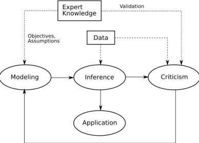
This thesis focuses on latent variable models developed according to the “Box’s loop” probabilis-tic pipeline [20], illustrated in Figure 2.1. This is an iterative loop process for data analysis, which consists of three fundamental stages: model formulation, inference, and model criticism. According to this scheme, we should first formalize our assumptions into a simple model to fit knowledge do-main of the problem at hand, including hidden structure which we believe exists in the data. Second, we can use an inference algorithm to approximate4 the posterior distribution and analyze the data under the assumptions encoded through the priors and likelihood. Finally, we should assess whether the analysis succeeds or fails, i.e., revise whether the model gives accurate predictions or insights that are consistent with current expert knowledge, and repeat the cycle if required.
Why nonparametrics? Most machine learning problems consist in learning an appropriate fixed set of parameters within a model class given the training data. Typically, practitioners fit several models with a different number of parameters, and use a separate validation set to determine the most adequate number of parameters. Determining appropriate model classes is referred to asmodel
2
Note that the Bayes theorem is a general expression for any two random variables. We here further incorporate an asymmetric interpretation of the theorem, which lies at the foundation of Bayesian statistics.
3This does not mean that the posterior distribution will be consistent, i.e., that its mean will tend to the true values.
Additional conditions would be necessary for this to hold.
4
Modeling Inference Criticism Application Data Expert Knowledge Objectives, Assumptions Validation
Figure 2.1: Box’s loop probabilistic pipeline for research. First, we formalize the problem, and include appropriate assumptions based on expert knowledge. Second, we perform inference to learn the posterior distribution of the hidden variables. We can then use the posterior, i.e., apply the model, to make predictions and explore the data. Third and last, we revise the model using expert knowledge, accounting for weaknesses and strengths, eventually repeating the Box’s loop if necessary.
selection in the literature [18]. Model selection is of fundamental concern for machine learning
practitioners, not only for avoidance of over-fitting and under-fitting, but also for discovery of the appropriate causes and structures underlying data. Some examples of model selection and adaptation include: selecting the number of clusters in a clustering problem, the number of latent features in a matrix factorization problem, or the complexity (degrees of freedom) of a certain function in nonlinear regression.
Addressing model selection by fitting multiple models of varying complexity is computationally expensive. Nonparametric models constitute an alternative approach where model complexity is also learned from data. While parametric models are fully characterized by a fixed number of parameters, the number of parameters in nonparametric models grows with the amount of training data [135]. Nonparametric approaches are memory-based, in the sense that the amount of stored information into the model is proportional to the number of observations. For instance, thek-nearest neighbors method is nonparametric in the sense that it classifies the unseen instance based on thekpoints in the training set which are nearest to it (we need to store the whole training set for classification).5
Also, fitting a Gaussian mixture model (GMM) with a fixed number of Gaussians is a parametric approach for density estimation. A nonparametric version would be the Parzen window estimator, which centers a Gaussian at each observation, and hence uses one mean parameter per
observa-5
Note that nonparametric refers to the nature of the method, it does not mean that the method has no parameters, e.g., thek-nearest neighbors has one parameterk.
2.2
Intuition behind Bayesian Nonparametric Models
Bayesian nonparametric (BNP) models made their debut in the 70s, with the seminal papers of Fer-guson [53] and Antoniak [12] among others,6. Although mathematically elegant, inference was too problematic at that time, so BNP models did not pick up much attention in the community until the 90s, thanks to the introduction of Markov chain Monte Carlo (MCMC) methods [59]. Around ten years later, variational inference made its appearance in the field [102], and allowed BNP models to further scale to higher amounts of data, making them even more popular in the 2010s [21, 42]. Recent advances in the field of deep learning have taken the main interest of the machine learning community, putting BNP models in the background. Although powerful, the spread of BNP models is still moderate, for computational complexity still remains an important drawback. Several lines of research address this issue, both from the perspective of MCMC approaches (by including adaptive subsampling or stochastic gradient dynamics) [11] or scaling up variational inference techniques via noisy stochastic gradients [90].
BNP models combine the benefits of Bayesian methods with the flexibility of nonparametric approaches [61]. Instead of specifying a closed-form model, BNP techniques place probability mass on an infinite range of models and let the inference procedure select those configurations that best fit the data, in order to provide competitive predictions or density estimations [143]. Thus, BNP models provide a useful tool for problems in which the number of unknown hidden variables is itself unknown and can be learned using standard Bayesian inference techniques. Given our prior beliefs, the posterior in a parametric model is constrained to a closed family, whereas BNP models allow for more flexible shapes in the posterior distribution. Although a BNP model is characterized by an infinite-dimensional parameter space, only a finite subset of the available parameters is used for any given finite dataset. This subset will generally grow with the dataset size.
6
De Finetti’s theorem (which will be described later) dates from the 30s [35] but this was not fully exploited in the context of BNP approaches until decades later.
An illustrative example. In order to get a better intuition for BNP models, let us consider a finite GMM and its non-parametric Bayesian counterpart. For simplicity, we will assume unknown mixture means and known covariance matrix, e.g.,Σ=σxIwhereIrefers to the identity matrix. LetX =
[x1,x2, . . . ,xN]>be the input matrix forN input observationsxn ∈ RD×1, wheren = 1, . . . , N.
A finite GMM ofKclusters assumes the following likelihood distribution:
p(x1,x2, . . . ,xN|Φ) = K
X
k=1
πkN(µk, σxI), Φ={(πk,µk)Kk=1}, (2.2)
whereΦrefers to the set of hidden variables, µk is the k-th cluster parameter (mean vector), and
πkis the mixture weight for clusterk. GivenX, our aim is to learn the distribution ofΦ. Inferring
the joint posterior distribution p(Φ|X) directly is an intractable problem which cannot be solved analytically. To address such issue, a common practice is to introduce an auxiliary cluster assignment variableznfor each observationxnthat indicates the mixture to whichxnbelongs, e.g.,p(xn|zn) =
N(µzn, σxI). Equation 2.2 can then be rewritten as:
p(x1,x2, . . . ,xN|Φ) = N
Y
n=1
p(xn|zn,µ1:K), Φ={(πk,µk)Kk=1, (zn)Nn=1}, (2.3)
If we now assume a prior distribution overΦ, we can write the complete joint probability as
p(x1,x2, . . . ,xN,Φ) = YN n=1 p(xn|zn,µ1:K)p(zn|πk) YK k=1 p(µk) p(π), (2.4) and formulate a sequential generative process forXsuch thatp(X|Φ)is given by (2.2) or (2.3),
π∼Dirichlet(a1, . . . , aK) (2.5) ∀k= 1, . . . , K µk ∼ N(µ0,Σ0) (2.6) ∀n= 1, . . . , N zn∼Categorical(π) (2.7) xn|zn∼ N(µzn, σxI). (2.8)
πrefers to the vector of mixture weights[π1, . . . , πK],µ0,Σ0 anda={a1, . . . , aK}are the model
Figure 2.2:Graphical representation for a finite GMM.Nodes in a circle are random variables, grey nodes are observed ones, and white nodes are unobserved variables. Model (hyper)parameters are not circled. An infinite GMM has the same graphical representation but replacingk= 1. . .∞.
distribution is equivalent to a Multinomial distribution with number of draws equal to one. In this example, we have two types of latent variables: global variables (πk andμk for each k-th
clus-ter) and local variables (one cluster assignmentznfor each observationxn). Figure 2.2 shows the
corresponding graphical representation for a finite GMM withKclusters.
In contrast, a non-parametric GMM allows for a potentially unbounded number of clustersK, and can be obtained by using an infinite-dimensional distribution over the parameter space, i.e., by replacing (2.5) and (2.6) jointly by a stochastic process called the Dirichlet process (DP). The generative formulation in this case is given by:7
G= ∞ k=1 πkδμk ∼DP(α, H) (2.9) ∀n= 1, . . . , N θn∼G (2.10) xn|θn∼ N(θn, σxI), (2.11)
whereθnis the observation-specific cluster mean vector corresponding to observationn(using the previous cluster assignment variables, θn = μzn), andGis a random measure corresponding to a realization of the DP which can be written as an infinite sum of sticks oratoms of weights πk at
locationsμk, wherek = 1, . . . ,∞and∞k=1πk = 1. A DP is a stochastic process parameterized
by a concentration parameterαand base measureH(further details can be found in Section 2.3.1). Figure 2.3 shows a draw example G ∼ DP(α, H), where H defines a distribution for the atom locations, e.g., in our particular example H =. N(μ0,Σ0), and α plays the role of an “inverse variance” parameter, such that small values of α result in fewer sticks with high weights, whereas bigger values ofα“spread” the probability mass all over, resulting in a bigger number of sticks with
Figure 2.3: A draw exampleGfrom a Dirichlet process. We only depict the sticks with highest weights, although the number of sticks in infinite. DrawingGis equivalent to independently drawing eachμk ∼H,
andπfrom a certainstick-breaking process, which will be introduced in 2.3.1.
smaller weights. GivenG, the generative process consists of sampling one local variableθnfor each data pointxn. SinceGis discrete with probability one, θnwill take repeated values in proportion
toπ, resulting in different clusters of observations. Even if the number of atoms inGis infinite, a dataset is ultimately finite, and thus, the number of non-empty clusters (locationsμk for which∃j
s.t.θj =μk) will be bounded. In a streaming application, sampling an observation-specific variable
θ∗for a new observationx∗could either return a cluster mean from which we have already sampled
before, or a completely new cluster with some probabilityπnewthat is proportional toα.
Generally speaking, the central idea behind BNPs is the replacement of classical finite-dimensional prior distributions with general stochastic processes, allowing for a potentially infinite number of pa-rameters, i.e., an open-ended number of degrees of freedom in the model [203]. Thus, BNP models rely on random measures to induce an infinite-dimensional distribution over the parameter space, which we will define more rigorously in the next section.
2.3
Random Measures
A random measureM can be understood as a stochastic process indexed by a sigma algebra. Let
(Φ,FΦ)be a measurable space, whereΦis a set, andFΦ is a σ-algebra overΦ, for instance Φis the real line andFΦrefer to the Borel sets. A random measure defines a distribution over measures on that measurable space; it corresponds to a collection of random variablesM(A) ∈ [0,∞), one for each setA ∈ FΦ. The expectation of a random measure is called the mean measure, which we denote byν(A)=. E[M(A)].
Completely random measures. A completely random measure (CRM) refers to a random measure such that the massesG(A1),G(A2), . . .assigned to disjoint subsetsA1,A2,. . . ∈ FΦ by a draw
Gfrom the CRM are independent random variables [105]. The class of CRM includes important stochastic processes such as the Beta process (BP), Gamma Process, Poisson Process, and the stable
G= ∞ X
k=1
πkδφk ∼CRM(ν), (2.12)
where (φk)∞k=1 is the set of atom locations, and(πk)∞k=1 is the set of atom weights, which do not
necessarily sum to one. IfP∞k=1πk = 1holds, this CRM is then referred to as normalized random
measure. Further details on CRMs can be found in [105].
Normalized random measures. Given a completely random measure G ∼ CRM(ν), we can construct a normalized random measure P based on an underlying probability measure on Φ as follows P = ∞ X k=1 πk P∞ j=1πj δφk ∼NRM(ν). (2.13)
The most common example of normalized random measure is the DP, which can be obtained by normalization of the Gamma Process. Distributions over probability measures are of great impor-tance in Bayesian statistics and machine learning, and normalized random measures have been used in many applications including topic modeling, image segmentation, or monitoring of genetic popu-lations [200, 204].
Exchangeability and De Finetti’s theorem Random measures are at the heart of BNP models via
theDe Finetti’s theorem. Indeed, the theorem establishes a link between random measures and the
so-calledexchangeabilityproperty of the data. An infinitely exchangeable sequence of observations
x1,x2, . . . ,xN is a sequence whose probability is invariant under finite permutationsρof the firstN
elements, for allN ∈N[54], i.e.,
p(x1,x2, . . . ,xN) =p(xρ(1),xρ(2), . . . ,xρ(n)), ∀N ∈N. (2.14)
8
In probability theory, a L´evy process is a stochastic process with independent, stationary increments, which can be viewed as the continuous-time analog of a random walk [105].
According to De Finetti’s theorem, any infinitely exchangeable sequencex1,x2, . . . ,xN can be
writ-ten as a mixture of i.i.d. samples as follows:
p(x1,x2, . . . ,xN) = Z φ N Y n=1 Q(xn|φ)P(dφ), ∀N ∈N, (2.15)
whereQ(·|φ)is a family of conditional distributions andP is a random measure overΦcalled the
De Finetti mixing measure(or directing measure).
For instance, ifP is a discrete random measure drawn from a DP, andQ(·|φ) =. N(φ, σxI), we
recover the example of the Gaussian mixture model described in Section 2.2. Also, ifP is a DP, andQ(·|φ)is the discrete probability distribution described by the probability measureφ, we obtain a distribution over exchangeable partitions known as the Chinese restaurant process (CRP) [6]. As another example, ifP is a BP andQ(·|φ) is a Bernoulli process, we obtain a distribution over ex-changeable binary vectors; such construction defines the so-called Indian buffet process (IBP) [206]. In the following, we describe the two basic random measures that will be used along this thesis, to-gether with their corresponding collapsed processes: the DP and the BP, giving rise to the CRP and IBP respectively.
2.3.1 Dirichlet Process
The Dirichlet process (DP) is a stochastic process whose realizations are random infinite discrete probability distributions [53]. Let G0 be a probability random measure on the measurable space
(Φ,FΦ). A random probability measureGover(Φ,FΦ)is said to be a DP if, for any finite measur-able partition(A1, A2, . . . , Ar)ofΦ, the random vector
G(A1), G(A2), . . . , G(Ar)
is distributed as a finite-dimensional Dirichlet distribution of the form
G(A1), G(A2), . . . , G(Ar) ∼DirichletαG0(A1), αG0(A2), . . . , αG0(Ar) . (2.16)
We then writeG∼DP(α, G0), whereG0 is referred to as the base measure (which is the expected value of the process) andα∈ R+is the concentration parameter, which plays the role of an inverse variance. Thus, the weak distribution of a DP, i.e., the set of all its finite-dimensional marginals follow a Dirichlet distribution. The first two cumulants of the DP are given by
E[G(A)] =G0(A), and Var[G(A)] =
G0(A)(1−G0(A))
with a countably infinite number of clusters. However, since the weightsπkdecrease exponentially
quickly, only a small number of clusters will be used to describe the data a priori. In fact, the expected number of mixtures grows logarithmically with the number of observations. In the DP mixture model, the actual number of clusters describing the data is not fixed, and can be automatically inferred from the data using the usual Bayesian posterior inference framework. The DP mixture model has been widely studied in the literature [12, 50, 124].
In the following, we describe other closely-related processes and explicit representations of the DP, including the stick-breaking process and culinary metaphor of the CRP. Explicit representations of stochastic processes directly describe a random draw from the stochastic process, rather than describing its distribution.
Stick-Breaking Representation
The discrete random measureGin (2.18) is uniquely determined by two infinite sequences,{πk}k∈N
and{φk}k∈N. As stated in [188], the stick-breaking representation of the DP generates these two
sequences by drawingφk ∼G0 independently, and by drawing a set of auxiliary variables(vk)∞k=1
such that
vk∼Beta(α,1), and πk =vk kY−1
`=1
(1−v`). (2.19)
Note that the sequence of atom weights{πk}k∈Nconstructed by (2.19) satisfiesP∞k=1πk= 1with
probability one. We write π ∼ GEM(α) if π is a random probability measure over the positive integers defined by 2.19 (GEM stands for the authors Griffiths, Engen and McCloskey) [153].
Figure 2.4 illustrates a sequential construction of the sequence{πk}k∈N. Starting with a stick of
unit length, at each iterationk= 1,2, . . . ,∞, a piece of relative lengthvkis “broken off” (relative
1 . . . k= 1 k= 2 k= 3 π1 π2 π3
Figure 2.4:Illustration of the stick-breaking construction for the DP.DrawingG∼DP(α, G0)is equiva-lent to drawingπ∼GEM(α)andφk∼G0,∀k= 1, . . . ,∞independently.
Chinese Restaurant Process
The CRP is typically found in the literature of DPs. This process defines a distribution on infinite partitions of the data [6], and takes the name from a standard culinary metaphor that vividly illustrates how the DP operates [204]. In this metaphor, the atom locationsφkare referred to as “dishes” in a
restaurant, and observations that are clustered together are viewed as customers sitting on the same table, therefore eating from the same dish. In this generative process, customers enter the restaurant one at a time, and they can either sit on an existing table, with probability proportional to the number of previous customers that are already sitting on that table, or open a new table, with probability proportional toα. In the latter case, they also sample a new dish from the prior, i.e.,φknew ∼H.
The implicit representation of the DP, which is closely-related to the CRP, is the P´olya urn scheme[19]. Letθ1, . . . , θN be a sequence of i.i.d. random variables distributed according toG. That
is, all variablesθnare conditionally independent givenG, and hence exchangeable. The successive
conditional distribution ofθngivenθ1, . . . , θn−1takes the form
θn|θ1, . . . , θn−1, α, G0∼ i−1 =1 1 i−1 +αδθ+ α i−1 +αG0. (2.20)
This expressions shows thatθnhas non-zero probability of being equal to one of the previous draws.
This leads to a “rich gets richer” effect, in which the more often a point is drawn, the more likely it is to be drawn in the future. Let{φk}Kk=1denote a sequence containing the unique values of variables
θn. By definingmkas the number of valuesθnwhich are equal toφk, we can rewrite (2.20) as
θn|θ1, . . . , θn−1, α, G0 ∼ K k=1 mk i−1 +αδφk + α i−1 +αG0. (2.21)
Note that, despite this “richer gets richer” effect, the probability ofθn being drawn fromG0 (and
k
tables at which the customers sit. Then-th customer sits at the tableφ
kwith probability proportional
to the number of customersmkalready seated there (in which case we setθn=φk), or sits at a new
table with probability proportional toα(therefore increasingKby one, drawing thenφ
K ∼G0, and
settingθn=φK).
Finally, let us explicitly relate the P´olya urn scheme to the CRP. For that, let us now introduce auxiliary random variablesz1, z2, . . . ,∞to indicate the assigned atom index of each random draw, e.g.,θn = φzn = φ
k. Compared to the P´olya urn scheme in which we considered the conditional
distribution of theactual colorof each new drawn ball, we now consider the colorindexindicating that color. In other words, the CRP describes the sequential probability of each cluster assignment variable, zn|z1, . . . , zn−1, α, G0 ∼ K k=1 mk i−1 +αδk+ α i−1 +αδknew. (2.22) wherek= 1, . . . , Kcorrespond to the atom indexes of the already observed clusters (colors that have already appeared in the P´olya urn model or non-empty tables in the CRP), andknewcorresponds to a
completely new index. The iterative process in Eq. 2.22 defines a distribution over infinite partitions. See Figure 2.5 for a sketch of the CRP. INDIANBUFFETPROCESS
... 2 10 6 7 9 3 1 4 8 5
Figure 2: A partition induced by the Chinese restaurant process. Numbers indicate customers (ob-jects), circles indicate tables (classes).
it is identical to the extended Polya urn scheme introduced by Blackwell and MacQueen 1973).
Imagine a restaurant with an infinite number of tables, each with an infinite number of seats.2The
customers enter the restaurant one after another, and each choose a table at random. In the CRP
with parameterα, each customer chooses an occupied table with probability proportional to the
number of occupants, and chooses the next vacant table with probability proportional toα. For
example, Figure 2 shows the state of a restaurant after 10 customers have chosen tables using this
procedure. Thefirst customer chooses thefirst table with probabilityα
α=1. The second customer
chooses thefirst table with probability 1
1+α, and the second table with probability
α
1+α. After the
second customer chooses the second table, the third customer chooses thefirst table with probability
1
2+α, the second table with probability
1
2+α, and the third table with probability2+αα. This process
continues until all customers have seats, defining a distribution over allocations of people to tables,
and, more generally, objects to classes. Extensions of the CRP and connections to other stochastic processes are pursued in depth by Pitman (2002).
The distribution over partitions induced by the CRP is the same as that given in Equation 5. If
we assume an ordering on ourNobjects, then we can assign them to classes sequentially using the
method specified by the CRP, letting objects play the role of customers and classes play the role of
tables. Theith object would be assigned to thekth class with probability
P(ci=k|c1,c2, . . . ,ci−1) = mk
i−1+α k≤K+
α
i−1+α k=K+1
wheremkis the number of objects currently assigned to classk, andK+is the number of classes for
whichmk>0. If allNobjects are assigned to classes via this process, the probability of a partition
of objectscis that given in Equation 5. The CRP thus provides an intuitive means of specifying a
prior for infinite mixture models, as well as revealing that there is a simple sequential process by
which exchangeable class assignments can be generated.
2.4 Inference by Gibbs Sampling
Figure 2.5: Illustration of the Chinese restaurant process. Circles correspond to tables in the restaurant, while numbers correspond to customers sitting on tables.
Hierarchical Dirichlet Process
The hierarchical Dirichlet process (HDP) is a well-known BNP prior which is useful for modeling grouped data [204]. The HDP is a distribution over a set of random probability measures. The process defines a set of random probability measuresGj (one for each group of data), and a global
random probability measure G. The global measure G is distributed as a DP with concentration parameterγ and base probability measureG0, i.e.,G∼DP(γ, G0). Hence, it can be written as
G= ∞ X
k=1
ρkδφk. (2.23)
The random measures Gj are conditionally independent givenG, and they are distributed as DPs
with concentration parameterαand base probability measureG, i.e., Gj ∼DP(α, G). SinceGis
a discrete probability measure with support at the points{φk}k∈N, each probability measureGj has
support on the same set of points and, therefore, we can write
Gj =
∞ X
k=1
πjkδφk. (2.24)
In other words, the atom weights9πjkare different for each groupj, but the atom locations are shared
across groupsj.
Let(A1, A2, . . . , Ar)be a measurable partition ofΦ. SinceGj ∼DP(α, G)for eachj, we have
by definition that the random vector Gj(A1), Gj(A2), . . . , Gj(Ar) is distributed as Gj(A1), Gj(A2), . . . , Gj(Ar) ∼DirichletαG(A1), αG(A2), . . . , αG(Ar) . (2.25)
This will be useful to establish the connection between the weightsπjkand the weights of the global
measure,ρk. Note that Eq. 2.24 defines an infinite mixture model for each group of observationsj.
Furthermore, all groups share the atom locationsφk(which do not depend onj), and they also share
statistical strength on the weightsπjk.
2.3.2 Beta Process
A BP is a CRM which is often used as a Bayesian nonparametric prior for sparse collections of binary features [206]. BPs are defined on an abstract measurable space(Φ,FΦ)and have the property that the mass of any particular atom lies in the interval [0,1]. The BP can be constructed based on a random measureΠ ∼ PP(ν) of a Poisson Process defined on (Φ×[0,1],FΦ× F[0,1]), whereν refers to its mean measureν(dφ, dπ) =απ−1(1−π)(α−1)dπP(dφ)[145]. The first dimension of
9
We use the notationπ = [π1, π2, . . .]to refer to the atom weights of the global probability measureG, andπj = [πj1, πj2, . . .]to refer to the atom weights of each group-level probability measureGj.
BeP(G). When the BP is marginalized out, we obtain the IBP [206]. Stick-Breaking Construction
The stick-breaking construction of the BP in [202] is an useful representation for some inference al-gorithms. In this construction, a sequence of independent Beta-distributed random variables{vk}k∈N
are used to obtain the atom weights{πk}k∈N. These are generated according to
vk ∼Beta(α,1), πk= k
Y
`=1
v`, (2.26)
resulting in a decreasing sequence of probabilitiesπk. This construction can be understood with the
stick-breaking process illustrated in Figure 2.6. Starting with a stick of length 1, at each iteration
k = 1,2, . . ., a piece is broken off at a pointvk relative to the current length of the stick. The
variableπkcorresponds to the length of the stick just “broken off”, and the other piece of the stick is
discarded. 1 . . . k= 1 k= 2 k= 3 ⇡1=v1 ⇡2=⇡1v2 ⇡3=⇡2v3
Figure 2.6:Illustration of the stick-breaking construction for the BP.
Indian Buffet Process
The IBP is a stochastic process defining a probability distribution over equivalence classes of sparse binary matrices with a finite number of rows and an unbounded number of columns [72]. Although the number of columns is potentially infinite, only a finite number of those will contain non-zero entries due to the finite nature of the observed data. Another important property of IBP-generated
matrices is that they are exchangeable both in rows and columns. The IBP can be derived taking the limit asK → ∞of a finite binary matrixZ∈ {0,1}N×K, whose elementsz
nk are distributed
according to:
πk∼Beta(α/K,1), znk ∼Bernoulli(πk), (2.27)
where πk is the probability of observing a non-zero value in column k, zn• is the n-th row for samplenandz•k is thek-th column of matrixZ. We say that a featurekis active for samplenif
znk = 1. WhenK → ∞, the above process is equivalent to the IBP. We denote:
Z∼IBP(α), (2.28)
whereαis the concentration parameter controling the a priori activation probability of new features. The expected number of active features per row is distributed according toPoisson(α)and the actual numberKof features with non-zero elements is distributed asPoisson α·PNi=1
1
i . The
param-eterα has thus an effect on both, the a priori number of columns inZand degree of sparseness of the matrix, e.g., a bigger value forαresults in a higher number of expected latent features and more active features per row a priori.
As discussed previously, the underlying De Finetti’s representation of the IBP is a mixture of BePs directed by a BP as follows:10
G∼BP(1, α, H) (2.29)
Zn·∼BeP(G), (2.30)
whereGis the directing measure, andH is the probability base measure for the BP [206]. The IBP can also be directly obtained by combining the previously described stick-breaking construction with an infinite collection of Bernoulli-distributed random variables (one for each atom) as:
vk ∼ Beta(α,1), πk= k Y i=1 vi, znk ∼ Bernoulli(πk). (2.31)
Similarly to the culinary metaphor for the CRP, there exists a sequential stochastic process that defines a conditional distribution p(znk|Z−nk) which can be illustrated using a new culinary
metaphor that gives the name to this stochastic process. Imagine an Indian restaurant whose buffet 10
Eq. 2.29 and 2.30 employ a common slight misuse of notation by ignoring the features’ position of the beta and Bernoulli processes.
ture activation probability, although any feature permutation will have the same probability given the exchangeability property over columns. The actual distribution over the equivalence matrixZis independent of the arrival order of customers entering the restaurant [202].
2.4
Inference Methods
The main computational problem in BNP modeling (as in most of Bayesian statistics) is computing the posterior distribution. For most interesting models, the posterior is computationally not tractable (not available in closed form), thus requiring inference algorithms to compute an approximation. The two most popular inference approaches are MCMC and variational inference techniques.
MCMC methods refer to iterative algorithms in which groups of latent variables are sampled given all the rest (such distributions are called the conditional distributions). This approach has asymptotic theoretical guarantees: it consists in defining a Markov chain on the different states of the hidden variables whose asymptotic distribution (equilibrium distribution) is known to converge to the posterior distribution. Samples obtained from this Markov chain will eventually correspond to samples from the posterior as the number of iterations tends to infinity [177]. A simple form of MCMC sampling is Gibbs sampling, where the Markov chain is constructed by considering the con-ditional distribution of each hidden variable given the rest of hidden variables and the observations. The CRP construction is particularly amenable to Gibbs sampling inference, as obtaining these con-ditional distributions is straightforward. A detailed survey of Gibbs sampling for inference in DP mixture models can be found in [140]. Gibbs sampling for the IBP is described in [72].
In contrast, variational inference resorts to transforming the inference problem into an optimiza-tion task [102]. The idea here is to approximate the posterior distribuoptimiza-tion by a simpler family of dis-tributions and searching for the member of that family that is closest to it (according to the Kullback-Leibler divergence). This is also equivalent to maximizing a certain lower bound on the marginal distribution of the data, called the “Evidence Lower Bound” (ELBO). Unlike MCMC methods,
vari-ational inference algorithms are not guaranteed to recover the posterior, but they are typically faster than MCMC, and convergence assessment is straightforward. These methods have been applied to DP mixture models [21] and IBP latent feature models [42].
2.5
Summary
In this chapter, we have given a gentle introduction to Bayesian nonparametric and intuition, in-cluding concepts such as exchangeability, De Finetti’s theorem, completely random measures and normalized random measures. We have presented the basic building blocks (stochastic processes) which will be used within this thesis, i.e., the Dirichlet process, and the Beta process, as well as the additional processes resulting from integrating the De Finetti’s mixing random measure in a Dirichlet process and a hierarchical Beta process–Bernoulli process construction: the Chinese restaurant pro-cess and the Indian buffet propro-cess. Finally, we have given an overview of the most common inference approaches to fit BNP models, i.e, to approximate the posterior distribution. The remaining chapters are devoted to our contributions.
3
Atom-Dependent Dirichlet Process
for Marathon Modeling
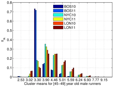
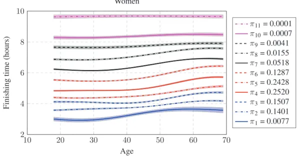
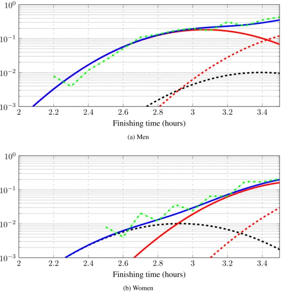
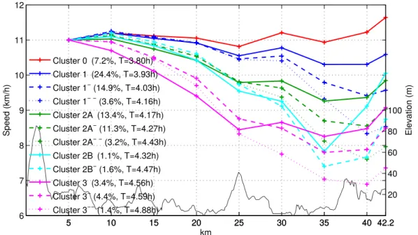
This chapter presents a novel application of Bayesian nonparametrics (BNPs) for density estimation of stratified data, with application to data from marathon runners. In particular, we make use of the dependent Dirichlet process (DDP) [125], which is a powerful tool that encompasses the Dirichlet process (DP) and the hierarchical Dirichlet process (HDP). However, the DDP is very general and it cannot be directly applied to data without additional constraints. Here, we specify a way to tie the parameters across groups using a Gaussian process (GP) [172], thus making the DDP a practical prior for our problem at hand. Additionally, we rely on the HDP to model intermediate running times for each runner, uncovering different running patterns within athletes. This model is also used to predict the finishing time in the race. Finally, we relate the proposed model to the literature of infinite mixture of experts (IMoE) in the context of non-linear regression [171].
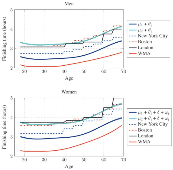
the only way that a participant can gain entry to the race, while other paths are available in New York, Chicago or London.1 Our objective is to propose a methodology that can be used to equalize entry requirements for different marathons, which vary considerably for one event to the next, as there is no widely accepted standard method to specify them. Furthermore, the world master of athletics (WMA) has an age-grading system for equalizing the finishing time according to the age and gender of athletes.2 They lobby for this measure to be taken into consideration for selecting the winners of each race, even though that procedure is based on world records, i.e., outliers that may not be very representative, or even realistic, for most races. Our method also provides an alternative way to reward runners fairly regardless of their age and gender.
Our approach consists in adapting a single-p dependent Dirichlet process (sp-DDP) to cluster the finishing time for each runner according to his/her age and sex [125]. We propose a Gaussian process to control how the clusters (representing marathon finishing time) change from one group to the next (different ages or gender). We find that the means of these clusters are directly comparable to the marathon entry requirements and the age-graded tables from the WMA. Additionally, direct comparisons for any finishing time are straightforward, since we find a full distribution for all ages and both genders. The sp-DDP can simultaneously deal with different races and/or the same race on different years, providing a unified ranking for all the races that may differ on elevation profile, temperature or humidity.
3.2
Dependent Dirichlet Processes
The DDP is a generalization of the DP that can be applied for clustering of groups of data [124]. For each groupj, we have an infinite mixture model of the form
Gj = ∞ X k=1 πjkδφjk, (3.1) 1
Complete information for each ma