King’s Research Portal
DOI:
10.1016/j.scitotenv.2018.08.122
Document Version
Peer reviewed version
Link to publication record in King's Research Portal
Citation for published version (APA):
Miller, T. H., Gallidabino, M. D., MacRae, J. R., Owen, S. F., Bury, N. R., & Barron, L. P. (2018). Prediction of bioconcentration factors in fish and invertebrates using machine learning. Science of the Total Environment. DOI: 10.1016/j.scitotenv.2018.08.122
Citing this paper
Please note that where the full-text provided on King's Research Portal is the Author Accepted Manuscript or Post-Print version this may differ from the final Published version. If citing, it is advised that you check and use the publisher's definitive version for pagination, volume/issue, and date of publication details. And where the final published version is provided on the Research Portal, if citing you are again advised to check the publisher's website for any subsequent corrections.
General rights
Copyright and moral rights for the publications made accessible in the Research Portal are retained by the authors and/or other copyright owners and it is a condition of accessing publications that users recognize and abide by the legal requirements associated with these rights. •Users may download and print one copy of any publication from the Research Portal for the purpose of private study or research.
•You may not further distribute the material or use it for any profit-making activity or commercial gain •You may freely distribute the URL identifying the publication in the Research Portal
Take down policy
If you believe that this document breaches copyright please contact [email protected] providing details, and we will remove access to the work immediately and investigate your claim.
1 PREDICTION OF BIOCONCENTRATION FACTORS IN FISH AND 1
INVERTEBRATES USING MACHINE LEARNING 2
Thomas H. Millera*, Matteo D. Gallidabinob, James R. MacRaec, Stewart F. Owend, 3
Nicolas R. Buryef, Leon P. Barrona* 4
5
aDepartment of Analytical, Environmental & Forensic Sciences, School of Population 6
Health & Environmental Sciences, Faculty of Life Sciences and Medicine, King’s 7
College London, 150 Stamford Street, London, SE1 9NH, UK. 8
bDepartment of Applied Sciences, Northumbria University, Newcastle Upon Tyne, NE1 9
8ST, UK. 10
cMetabolomics Laboratory, The Francis Crick Institute, 1 Midland Road, London, NW1 11
1AT, UK. 12
dAstraZeneca, Global Environment, Alderley Park, Macclesfield, Cheshire SK10 4TF, 13
UK. 14
eDivision of Diabetes and Nutritional Sciences, Faculty of Life Sciences and Medicine, 15
King’s College London, Franklin Wilkins Building, 150 Stamford Street, London, SE1 16
9NH, UK. 17
fFaculty of Science, Health and Technology, University of Suffolk, James Hehir 18
Building, University Avenue, Ipswich, Suffolk, IP3 0FS, UK. 19
20
*Corresponding authors 21
Email: [email protected] (Tel: +44 20 7848 4978) or [email protected]; 22
(Tel.: +44 20 7848 3842) 23
24 25
2 GRAPHICAL ABSTRACT 26 27 28 29
3 Abstract
30
The application of machine learning has recently gained interest from ecotoxicological 31
fields for its ability to model and predict chemical and/or biological processes, such as 32
the prediction of bioconcentration. However, comparison of different models and the 33
prediction of bioconcentration in invertebrates has not been previously evaluated. A 34
comparison of 24 linear and machine learning models is presented herein for the 35
prediction of bioconcentration in fish and important factors that influenced 36
accumulation identified. R2 and root mean square error (RMSE) for the test data (n = 37
110 cases) ranged from 0.23 – 0.73 and 0.34 – 1.20, respectively. Model performance 38
was critically assessed with neural networks and tree-based learners showing the best 39
performance. An optimised 4-layer multi-layer perceptron (14 descriptors) was 40
selected for further testing. The model was applied for cross-species prediction of 41
bioconcentration in a freshwater invertebrate, Gammarus pulex. The model for G. 42
pulex showed good performance with R2 of 0.99 and 0.93 for the verification and test 43
data, respectively. Important molecular descriptors determined to influence 44
bioconcentration were molecular mass (MW), octanol-water distribution coefficient 45
(logD), topological polar surface area (TPSA) and number of nitrogen atoms (nN) 46
among others. Modelling of hazard criteria such as PBT, showed potential to replace 47
the need for animal testing. However, the use of machine learning models in the 48
regulatory context has been minimal to date and is critically discussed herein. The 49
movement away from experimental estimations of accumulation to in silico modelling 50
would enable rapid prioritisation of contaminants that may pose a risk to environmental 51
health and the food chain. 52
Keywords modelling, PBT, pharmaceutical, bioconcentration, BCF, machine 53
learning 54
4 Introduction
55
Both terrestrial and aquatic environments experience pollution from a wide 56
range of chemical contaminants. The presence of these contaminants is a cause for 57
concern as they may elicit adverse effects to environmental and public health. 58
Bioaccumulation of chemicals is critically important for understanding the risk of 59
chemicals in the environment. The complexity of confounding factors that affect uptake 60
make simple relationships that can confidently predict the accumulation elusive; but it 61
may not have to be that way. 62
Live animal exposure studies are currently the norm, using many hundreds of 63
fish for each assessment [1]. Across the European Union (EU), various guidelines 64
have been established for industry to minimise the risk posed by their chemical 65
products. For pharmaceuticals in the EU this is regulated by the European Medicines 66
Agency (EMA) and for other chemicals substances the regulations are outlined by the 67
Registration, Evaluation, Authorisation and restriction of CHemicals (REACH) [2, 3]. 68
According to REACH, any manufacturer of a chemical that exceeds quantities of 10 69
tonnes per annum must submit a chemical safety assessment (CSA). For 70
environmental risk assessment, part of the CSA includes persistence, 71
bioaccumulation and toxicity (PBT) assessments. Alternatively, for pharmaceuticals 72
environmental risk assessment (ERA) follows an initial screening (Phase I) where 73
physico-chemical properties of the compound are determined (e.g. logP) and the 74
expected exposure is estimated. The Phase I exposure estimation is calculated as the 75
predicted environmental concentration (PEC). If the PEC is >0.01 µg L-1 then the 76
pharmaceutical must undergo further testing to assess environmental fate and toxicity. 77
However, it should be noted that substances with a logP >4.5, will trigger a PBT 78
assessment (following REACH guidelines) regardless of the Phase I PEC. 79
5 For PBT assessments, existing available screening data and prior assessment 80
information are used to determine whether a chemical is bioaccumulative (B) or very 81
bioaccumulative (vB) by estimation of a bioconcentration factor (BCF) or 82
bioaccumulation factor (BAF). Currently, pharmaceuticals are not restricted or 83
replaced as would normally be defined under REACH. Furthermore, whilst PBT 84
assessments are implemented, the persistence and bioaccumulation outcome of 85
these assessments are not taken into consideration for authorisation purposes, as no 86
legal provisions specifically cover persistent, bioaccumulative and toxic substances 87
for pharmaceuticals [4]. 88
Laboratory testing for PBT brings with it a significant level of planning, quality 89
control and cost [1]. Therefore, in silico methodologies to predict BCF or BAF offers a 90
potential advantage to more intelligently use data to characterise potential exposure 91
and risk. Quantitative Structure Activity Relationships (QSARs) are becoming 92
increasingly popular within ecotoxicological fields as they represent, perhaps, the only 93
realistically feasible scenario to assess the environmental risk of the several thousand 94
chemicals that are available on the market [5]. In addition, such models can be used 95
to ethically reduce or replace animal testing and falls under the replacement, reduction 96
and refinement (3Rs) framework [6]. Further, effective in silico models could also be 97
utilised to help shape future drugs in terms of ‘green by design’ ambitions [7]. 98
More recently, more complex machine learning-based QSAR models involving 99
artificial neural networks (ANNs), tree-based learners or support vector machines 100
(SVMs) have been used to model BCF in fish [8-11]. However, several variations of 101
machine learning-type models exist and wider applications of such models for 102
bioaccumulation prediction have not yet been evaluated to identify any added benefits. 103
Furthermore, current QSAR models have only been applied to modelling fish 104
6 bioaccumulation data and do not incorporate pharmaceutical data. The potential for 105
application to other taxa such as invertebrates is also non-existent, mainly due to a 106
shortage of available data. 107
The aim of this work was to develop and critically evaluate several machine 108
learning-based modelling tools for prediction of bioconcentration factor (BCF) in both 109
a fish (Cyprinus carpio) and an invertebrate species (Gammarus pulex) for the first 110
time. An open access fish BCF dataset was used in the first instance to build and 111
compare 24 different models for 352 different compounds. Subsequently, the best 112
model was applied to both a set of fish and invertebrate BCF data to assess its 113
potential for cross-species prediction. The invertebrate dataset also contained mainly 114
pharmaceuticals. In parallel, independent models were developed ab initio on a 115
smaller set of invertebrate BCF data alone to assess the degree of commonality with 116
the model developed on fish BCF data. Finally, the importance of molecular 117
descriptors to understand the potential for a chemical to accumulate in biota was 118
assessed. The use of such rapid and flexible modelling approaches is now critical to 119
support the 3Rs, aid greener design and to help meet the demand for PBT 120
assessments of potentially large numbers of compounds, which could be expanded to 121
new and emerging environmental contaminants across different species. 122
123
Materials and Methods 124
Dataset generation and pre-processing 125
Bioconcentration factors were collated from the European Chemical Industry 126
Council Long-range Research Initiative (Cefic LRI) project EC07 in collaboration with 127
European Academy for Standardisation e.V (EURAS) which established the BCF gold 128
standard database across multiple fish species and is freely available at 129
7 http://ambit.sourceforge.net/euras/. BCFs were down-selected to reduce variability 130
between different species and experimental conditions within the database. The BCF 131
data used herein were specific to C. carpio and were included by the Chemicals 132
Inspection and Testing Institute [12]. Out of all BCF data, this sub-selection resulted 133
in the largest dataset with a single fish species (n=352) for modelling purposes. The 134
reported BCFs represented whole-body values only and included pigments, 135
pesticides, fungicides, herbicides, insecticides, polyaromatic hydrocarbons (PAHs) 136
and polychlorinated biphenyls (PCBs), organochlorines, nitroaromatics, alkylphenols, 137
aromatic hydrocarbons, organosulfurs and organotins. Approximately 36 % of the 138
dataset contained ionisable compounds (estimated from ACD labs, Percepta 139
software). The invertebrate BCF dataset (n=34) was collated from literature reported 140
data [13-17] for the benthic freshwater organism, G. pulex. This species was selected 141
as there was a relatively large amount of BCF data available when compared with 142
other invertebrate species. For these, BCF data were only available for 143
pharmaceuticals and pesticides and, again, represented whole-body values. 144
Simplified molecular input line entry system (SMILES) strings were generated 145
for each compound using Chemspider (Royal Society of Chemistry, UK). Molecular 146
descriptors were generated from SMILES strings using Parameter Client (Virtual 147
Computational Chemistry Laboratory, Munich, Germany), and ACD Labs Percepta 148
(Advanced Chemistry Development Laboratories, ON, Canada). Approximately 450 149
descriptors were initially generated covering constitutional, topological, geometrical 150
and physico-chemical properties. The fish and invertebrate datasets were pre-151
processed to remove any zero variance descriptors or descriptors that were 152
erroneous. All BCF data used for modelling was log transformed for improved 153
predictive accuracy. 154
8 155
Feature selection 156
Descriptors were down-selected using three different feature selection 157
algorithms, the first of which was a genetic algorithm (GA). The GA parameters were 158
set to population = 500, generations = 250, mutation rate = 0.1 and cross-over rate = 159
1. The remaining two selection methods were part of stepwise regression which 160
included a forward selection algorithm (FA) and backwards selection algorithm (BA). 161
The feature selection algorithms used a generalised regression neural networks 162
(GRNN) to monitor the error associated with the selected descriptors, where descriptor 163
sets were optimised when the error showed no improvement. The use of GRNN for 164
descriptor selection is very fast and requires minimal processing power. The 165
performance of each feature selection algorithm was characterised by then testing 166
several thousand neural networks and evaluating the predictive performance of the 167
models based on the error of the predictions. The best feature selection method was 168
the GA, which resulted in the down-selection of descriptors to a total of 14 that included 169
6 topological descriptors; radial centric information index (ICR), Narumi harmonic 170
topological function (Hnar), ramification index (Ram), superpendentic index (SPI), 171
spanning tree number (STN), topological polar surface area (TPSA), 4 constitutional 172
descriptors; number of hydrogens (nH), number of carbons (nC), number of nitrogens 173
(nN), molecular weight (MW), 3 electrotopological descriptors; maximal 174
electrotopological negative variation (MAXDN), maximal electrotopological positive 175
variation (MAXDP), mean atomic Sanderson electronegativity (Me) and 1 physico-176
chemical property; the octanol-water distribution coefficient (logD) (See SI, Table S3). 177
178
Modelling approaches 179
9 Two different software packages were used to assess the applicability of 180
several in silico models in predicting bioconcentration. Trajan 6.0 (Trajan Software 181
Ltd., Lincolnshire, UK) was used to build and evaluate artificial neural networks. In 182
addition, this software was also used for the feature selection and the same 183
descriptors were used in both modelling software packages. Models developed and 184
optimised in Trajan included generalised regression neural networks (GRNN), radial 185
basis function networks (RBF) and 3-/4-layer multilayer perceptrons (MLP). Training 186
of the MLPs used two training algorithms referred to as back propagation (BP) and 187
conjugate gradient descent (CGD), models were trained for 100 iterations. The 188
optimised model was a four-layer MLP. The first and fourth layers were the inputs 189
(molecular descriptors) and outputs (logBCF), respectively. The second and third 190
layers (hidden layers) contained 14 and 10 nodes, respectively. Regularisation was 191
performed with the use of early stopping to prevent over-training of the dataset. 192
Parameter tuning was performed by changing the number of hidden layers and nodes 193
and assessing the model performance on the verification and test subsets. The 194
subsets of cases presented to the neural networks were split so that 242 compounds 195
(70 %) were used for training, 55 compounds (15 %) for verification and 55 compounds 196
(15 %) for testing the networks. Normalisation of the input features showed no 197
improvement in performance of the networks and training was performed without 198
centred or scaled descriptors. 199
In the second software package, modelling was performed using the R 200
statistical computing language (freely available from https://www.r-project.org). Here, 201
19 predictive models from different kinds of learner categories including both linear 202
and non-linear models were trained and tested. These included, ordinary least-203
squares regression (OLM, package: stats), partial least-squares (PLS, package: pls), 204
10 ridge regression (RR, package: elasticnet), elastic net (EN, package: elasticnet), 205
quantile regression with LASSO penalty (QRL, package: rqPen) multivariate adaptive 206
regression splines (MARS & B-MARS, package: earth), k-nearest neighbours 207
regression (KNN, package: caret), extreme learning machines (ELM, package: 208
elmNN), support vector machines with radial basis function (SVM-R, package: 209
kernlab) and polynomial (SVM-P, package: kernlab) kernels, random forest exploiting 210
classification and regression trees (RF-CART, package: randomForest) and 211
conditional inference trees (RF-CIT, package: party) algorithms as base learners, 212
boosted trees (BT, package: gbm) and Cubist regression (CR, package: Cubist). MLPs 213
(3-5 layers) with 1 hidden layer (ANN-1HL, package: nnet), averaged 1 hidden layer 214
(ANN-a1HL, package: nnet), 2 hidden layers (ANN-2HL, package: RSNNS) and 3 215
hidden layers (ANN-3HL, package: RSNNS) were also tested. For this modelling 216
approach, the same molecular descriptors and logBCF were used again as input and 217
output variables. The dataset was split into two subsets, training data (70 %) and test 218
data (30 %). Normalisation of the data was required for the modelling application and 219
the dataset was both centred and scaled. Parameter tuning was performed by 220
resampling of the training subset following a 10-fold cross-validation scheme repeated 221
five times and implemented through the caret package. Performance of each model 222
was assessed from the root-mean square error (RMSE) and the correlation coefficient 223
(R2). The best model for each regression method was then selected, retrained on the 224
entire training dataset and used to predict cases in the test dataset. Final datasets 225
used for modelling the optimised models are given in the SI (Table S1 & S2). The 226
finalised models were all tested according to OECD guidelines [18] for QSAR model 227
validation. 228
11 Results and Discussion
230 231
Down-selection of input features for modelling BCFs in fish 232
The down-selection of the input features was assessed using three different 233
feature-selection algorithms. Stepwise methods that included forwards or backwards 234
selection (FA/BA) reduced the number of descriptors from 180 down to 72, whilst the 235
GA reduced the number of descriptors to 66. The GA showed better correlation 236
between selected descriptors with logBCF compared to stepwise algorithms (Figure 237
S1). For both BA and FA, the selection process converged to the same local minima 238
indicating that there was no difference in using either algorithm. The improved 239
performance of the GA is due to selection of descriptors from multiple points in the 240
descriptor space, as opposed to FA or BA that start selection from a single point. Thus, 241
approaching global minima is more likely to arise when using the GA over stepwise 242
selection methods. 243
From the 66 descriptors selected by the GA, the top 22 descriptors plus an 244
additional two user curated descriptors were selected for further modelling (See SI, 245
Table S3). These additional descriptors were logD and number of hydrogen acceptor 246
groups (nHAcc) and were chosen for their previously demonstrated influence on 247
accumulation in biota [19, 20]. All descriptors were then tested across several 248
thousand MLPs (three and four-layer) where the Trajan software sub-selected the best 249
from the group of 24 descriptors based on model performance (MLPs yielded the best 250
performance over other model types in terms of R2 and RMSE). The descriptors were 251
down-selected to a total of 14 that showed relatively good performance across MLPs 252
tested and were subsequently used in both modelling approaches discussed herein 253
(Table S3). Given the scale of BCF data used for training (n=242), the 5:1 Topliss 254
12 threshold set out by the OECD guidelines [18] for the ratio of numbers of cases to 255
descriptors was acceptable at 17:1. 256
257
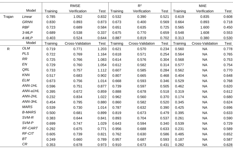
Comparison of model performances for prediction of fish BCFs 258
The results of both modelling approaches are shown in Table 1. For models 259
trained in R, the highest RMSE values were observed for OLM (1.203), followed by 260
PLS (1.164) and then QRL (1.112). The relatively poor performance of such linear 261
models may be expected as modelling such a biologically complex process is not likely 262
to follow linear relationships using simple molecular descriptors. Even with well-263
studied descriptors, such as logP, there is a non-linear trend with accumulation over 264
a specific threshold (generally, logP >6) [21]. However, when used as a sole 265
descriptor, logP may exclude processes that are also important for accumulation. For 266
example, elimination and metabolism rates may impact net accumulation as well as 267
more specific physiology such as carrier mediated transport and protein binding [22] 268
will also influence accumulation, especially for emerging contaminant classes such as 269
pharmaceuticals. By comparison, better performance was achieved using higher 270
complexity models. The lowest RMSEs were observed for RF-CART (0.771), followed 271
by BT (0.789) and RF-CIT (0.821), i.e. three tree-based machine learners. Next, ANNs 272
and SVMs performed very similarly to tree learners, e.g. SVM-R (0.841), ANN-a1HL 273
(0.859) and ANN-3HL (0.880). 274
Models tested in Trajan showed particularly good performance, in comparison 275
to those built in R. The lowest RMSE value was observed for a 4-layer MLP (0.524), 276
followed by 3-layer MLP (0.538), RBF (0.689), GRNN (0.893) and Linear (1.052). In 277
absolute terms, definitive conclusions cannot be drawn from direct comparison of 278
modelling approaches (i.e., Trajan vs. R), as tuning and training methods between 279
13 modelling software packages are slightly different. However, overall results converged 280
to support the higher reliability of non-linear approaches for modelling logBCF from 281
molecular descriptors. 282
Model complexity does not necessarily mean better predictive performance by 283
default, as several non-linear machine learners did not perform well at all. These 284
included ELM and SVM-P, where the RMSE values observed on the test set were >1. 285
Although ELM is a feedforward neural network, the weights associated with the 286
neurons in the network are not updated and thus the initialisation of the network is a 287
random selection of weights that may not model the output reliably. The EN 288
outperformed QRL and RR models, where the EN is a combination of the penalties 289
(L1 and L2 regularisation) used by both models that usually leads to better predictive 290
performance. The RR model RMSE for the test set data was also lower than the RMSE 291
for the QRL model. This can be observed when comparing RR and QRL methods, as 292
the penalty associated with LASSO can lead to the omission of highly correlated 293
covariables and thus lead to lower model robustness. 294
Limitations of predictive performance may also stem from the raw data. For 295
example, the dataset used herein did not report individual experimental pH, but instead 296
reported a range from 6.0 to 8.5. Therefore, descriptors such as logD that require pH 297
data may become limited and especially where molecular pKa lies within this 2.5 pH 298
unit range. LogD has been shown in several works to influence uptake and 299
accumulation [23-25]. As a compromise, we calculated logD at pH 7, but this may have 300
been different to the exact experimental pH and may have added to predictive 301
inaccuracy across the whole analyte set. Lastly, it is also likely that BCF/BAF 302
prediction will be influenced by variance in biotic factors such as ventilation rates, age, 303
14 genetic factors and metabolism and lay beyond our ability to determine in more detail 304
[26, 27]. 305
MLP models trained in Trajan offered the best performance. Consequently, this 306
model was chosen for further investigation in line with the OECD validation guidelines 307
to assess validity of QSAR modelling. The mean absolute error (MAE) corresponded 308
to 0.38 logBCF units for the verification subset (internal validation set) and 0.53 309
logBCF for the test subset (external validation set), as shown in Table 1. The RMSE 310
for verification and test subsets were 0.524 and 0.644, respectively. The predictive 311
performance of this model was better or comparable to all models in the literature that 312
have attempted to model accumulation processes. Dearden and Shinnawei [28] used 313
a linear QSAR approach to predict BCFs for 135 chemicals with an R2 of 0.637 and 314
RMSE of 0.661 logBCF units. Another QSAR model by Sahu and Singh [29] used 315
multiple linear regression to predict BCFs for 131 organic compounds with a RMSE of 316
0.556 log units. However, this model was not validated against a test subset and 317
therefore generalised applicability of the model performance is arguably limited. 318
In alternative approaches to linear QSAR models, other machine learning 319
approaches have also been reported [8-10]. A MLP predicted BCFs for 9 test 320
compounds with an average absolute error of 0.33 ±0.22 log units [8]. Whilst the errors 321
were low, too few compounds were tested to provide a reliable assessment of its 322
generalisability. In another approach, Zhao et al., [10] used SVM, RBF and MLR 323
models individually. Better performance was observed when two RBF models (using 324
different descriptors) were combined into a ‘hybrid’ model to predict logBCF. The 325
developed model showed an R2 of 0.6917 for an external test set with a reported 326
RMSE of 0.69 logBCF units for 119 compounds showing similar performance to the 327
fish-based MLP presented here, using a single MLP. The hybrid model also showed 328
15 a limitation in the training set, where several cases were not modelled correctly 329
between the ranges of logBCF 4 to 5 and was observed by a plateau in the regression 330
analysis. 331
332
A remark on outliers and the applicability domain 333
Training and testing of all models led to the observation of several common 334
outliers. The reason for poor prediction for such cases may stem from under 335
representation in the dataset used for modelling. The spread of input and output data 336
between training and validation subsets showed that there was no significant 337
difference between the spread or skew of the data (Figure S2). However, using PCA 338
analysis and distances between the descriptor spaces there were several cases that 339
did not cluster well with the remaining data (Figure 1a). For example, logBCF for 340
perfluorotributylamine was predicted poorly across the majority of trained models. The 341
use of PCA and descriptor data spacing in this way enabled characterisation of the 342
applicability domain (AD) for a given model. A threshold may then be used to 343
determine cases that fall outside the domain and are likely to have higher predictive 344
error (Figure 1b) [30, 31]. 345
According to the OECD QSAR model validation guidance [18], consideration of 346
models for regulatory purposes must be associated with a defined domain of 347
applicability under Principle 3. However, one key consideration in the use of distance-348
based ADs is that input descriptors are not used equally by the model [32]. Therefore, 349
such ADs may not accurately identify those cases having a greater predictive error in 350
every case. This was observed for outliers in the PCA analysis, but where logBCF was 351
predicted relatively well and vice versa. For example, di-2-naphthyldisulfide was not 352
an outlier in the AD but was poorly predicted across all models. On the other hand, 353
16 pigment yellow-12 was an AD outlier, but logBCF was predicted well by the majority 354
of models. 355
Poor predictive accuracy for molecularly similar compounds could be also 356
caused by other factors such as poor quality raw data or too few representative training 357
cases for the model to learn from. It has been shown previously that experimental BCF 358
data can vary from 0.42 to 0.75 log units [9, 33, 34]. Nevertheless, even with the 359
limitations associated with defining an AD, it is useful and important to identify any 360
cases that might not be reliably predicted so that rapid prioritisation of compounds can 361
begin. Only for these cases, may it then be appropriate to revert to experimental 362
testing. 363
364
Machine learning in a regulatory context 365
Several of the developed machine learning tools in Table 1 showed potential 366
for the replacement and reduction in animal use. However, it is important to recognise 367
the complexities of machine learning approaches from the outset, especially where 368
they are intended for use in regulation. Under Principle 2 of the OECD guidelines, 369
models used in this way must be based on “unambiguous algorithms”. In particular, it 370
is highlighted that two significant limitations exist regarding artificial neural networks, 371
for example. These are: (a) the necessity for large (BCF) datasets to develop suitable 372
models (which do not exist for some classes of compounds, like pharmaceuticals) and 373
also (b) that these types of machine learning tools are more ambiguous than other 374
types of model, especially those that are linear in nature. For the latter, the guidance 375
is vague concerning appropriateness of ANNs for use under this specific principle but 376
infers that it is an acceptable limitation. Furthermore, the definition of an unambiguous 377
algorithm is in fact ambiguous and should be further refined to prevent confusion to 378
17 the reader. This principle could be applied in different ways to different models and 379
may cover the generation of molecular descriptors, the feature selection algorithms 380
used, the learning process (for machine learners where the ambiguity lies) and the 381
final model [35]. The majority of the literature seems to have focused on linear models 382
perhaps as a result, mainly to aid in mechanistic understanding and to allow expert 383
interpretation of individual chemicals to provide extra assurance in predicted data 384
(linked to Principle 5). 385
Principle 5 of the OECD guidelines relates to mechanistic interpretability of 386
QSAR models (if possible). This can be considered a limitation for machine learning 387
algorithms if the aim is to achieve an interpretable model, such as would normally be 388
expected of linear models such as OLS or PLS regression. The OECD guidelines also 389
remain vague regarding mechanistic interpretation of machine learners. However, 390
whist linear relationships may not be apparent, descriptor sensitivity analyses can 391
indicate the importance of individual descriptors and thus enables interpretation of 392
factors that influence the modelled process. Bioconcentration processes are not 393
simple and extensive datasets are extremely impractical to curate experimentally. 394
Therefore, complex non-linear models may provide a more rapid solution to regulatory 395
decision-making meantime. Therefore, we suggest that guidelines for QSAR model 396
validation need to be expanded to better define the scope of applicability of all the 397
different types of machine learning tools and their fitness for purpose in a regulatory 398
context. 399
For PBT testing, the same regulations are triggered when a threshold for 400
bioaccumulation is reached, regardless of the extent to which the threshold is 401
exceeded. Thus, if the value is classified within the correct category of non-402
bioaccumualtive (nB), bioaccumulative (B) or very bioaccumulative (vB), the model will 403
18 be useful in the context of PBT assessments. Variability in measurement can arise 404
from kinetic modelling approaches [17], biological/physiological variability (age, health, 405
lipid content etc.) [27, 36-39] and experimental conditions (pH, temperature, etc.) [23, 406
40]. As such, reported BCFs have been shown to differ by 1-2 orders of magnitude 407
even within the same species [27]. 408
The 4-layer MLP here showed a correct classification rate of 90 % across the 409
verification and test subsets. The 10 % misclassification of cases was split to 6 % of 410
cases predicted as false negatives and 4 % of cases predicted as false positives (See 411
SI, Figure S3). This is consistent with the hybrid model developed by Zhao et al. which 412
has shown classification accuracies ranging from 91 % to 98 % [9, 10]. It is possible 413
that using QSARs for classification instead of regression analysis may improve the 414
accuracy and without the need for the application of a bias. This would be particularly 415
suitable for bioaccumulation assessments where only a threshold value determines 416
the level of regulation enforced. 417
Some studies have reported the application of models for classification of 418
bioaccumulation thresholds, with accuracies ranging from 84.5 – 91.1 % (depending 419
on model type) [41] and 91.7 % [11]. The authors that used tree-based learners also 420
used these models for quantitative prediction achieving RMSE of 0.554 and R2 of 421
0.836 on the test set data [11]. The models tested across the literature have tended to 422
achieve similar performance for both classification and prediction. The agreement in 423
performance between different works and the comprehensive model evaluation here, 424
support that in silico methods should be adopted for chemicals where environmental 425
uptake data are limited to enable flexible, cheap and rapid PBT assessment for 426
compound prioritisation. Furthermore, it suggests that the use of chemical descriptors 427
may only be able to achieve a certain level of predictive or classification performance 428
19 for modelling approaches where other variables become important as mentioned 429
above. 430
431
Can the developed model be used for cross phylum prediction? 432
There is little understanding of whether accumulation will be similar across the 433
invertebrate phylum. The dominant site of uptake for waterborne micropollutants in 434
fish is across the gills and therefore accumulation across taxa may be significantly 435
different for differing modes of respiration. Other factors such as size, enzyme 436
speciation and lipid content may also influence the accumulation potential [27]. The 437
optimised model for fish was applied to the prediction of logBCF in a freshwater 438
invertebrate, Gammarus pulex (Figure 3a). The accumulation data in G. pulex 439
predominantly covered pharmaceuticals and pesticides. The fish-based MLP showed 440
relatively low predictive performance for the invertebrate accumulation factors. The 441
correlation between observed and predicted BCF was R2 0.3295 with a MAE of 0.80 442
±0.65 log units, which indicated that the model generalisations between species were 443
limited. The largest predictive error was for the compound imipramine that was 444
overestimated by 2.7 logBCF units. This compound in a previous study had 445
considerable variation in the estimated BCF (212 – 4533) depending on the method 446
of estimation used [17]. 447
A significant difference in BCFs between trophic levels has been shown with 448
higher trophic levels displaying increased BCFs [42]. This trend would suggest that 449
the BCF predictions of the invertebrates might be overestimated but the opposite was 450
observed (62 % of cases were underestimated). In addition to the biological complexity 451
between species, another confounding factor to affect the predictive accuracy and 452
generalisability is the compound class. The fish model included no pharmaceutical 453
20 compounds whereas the invertebrate BCF data contained 18 cases (~53%). 454
Inspection of the molecular similarity between the datasets indicated that the 455
invertebrate and fish datasets were dissimilar (Figure S4). Thus, the bioconcentration 456
potential may not follow the same relationships with neutral hydrophobic organic 457
contaminants. 458
The fish-based model was subsequently reinitialised and trained on the 459
invertebrate dataset only (using the same descriptors) (Figure 3b). The invertebrate 460
model showed good correlation with R2 of 0.9605 with 0.972 for the training set, 0.9932 461
for the verification set and 0.9323 for the test set. The model demonstrated good 462
accuracy across the verification and test subset with a MAE of 0.07 ±0.08 logBCF 463
units for the verification set and 0.29 ±0.27 logBCF units for the test set. The 464
successful retraining of the model to invertebrate data suggests that case 465
representation (i.e. compound class) is likely to limit models that are applied across 466
taxa. An alternative approach to overcome this could involve development of a model 467
with two or more outputs to represent different species, but commonality in BCF cases 468
would be required for both species. Whilst the predictive accuracy of the retrained 469
model was very good, it is also limited by the small number of cases used. 470
Generalisability is also likely to be limited given the ratio of cases to descriptors 471
(Topliss ratio of ~2.5:1) Nevertheless, and as new BCF data emerges, this approach 472
holds excellent potential by using the same molecular descriptors for BCF predictions 473
in two very different species. In addition, to using the fish-based model to predict 474
invertebrate BCFs we also used the invertebrate-based model to predict fish BCFs of 475
pharmaceuticals reported in the literature (Figure S5). The invertebrate model was 476
able to predict BCFs within the reported range for 45 % of the compounds selected (n 477
= 11). The remaining compounds, with the exception of sertraline and gemfibrozil, 478
21 were predicted relatively well even though they were not within the reported ranges. 479
Sertraline is an interesting case as although it has not shown very high 480
bioconcentration in fish (BCFs: <1 – 626) [43-47] there have been reported BCF values 481
of up to 32,022 in invertebrates (namely, Lasmigona costata [48] and 990 in Planorbid 482
sp. [49]). As the model used here was trained on BCFs from an invertebrate species, 483
it may not correlate well with fish BCF data, suggesting that cross-phylum predictive 484
modelling may be limited by both case representation and biological variation. 485
However, as the models here used the same descriptors this enables flexibility in 486
retraining optimised models and inevitably as more BCF data is generated for the 487
same compounds in different species, this technology could be used to map 488
accumulation across taxa more effectively. It is critically important to understand 489
uptake (internal concentration) across taxa as the conservation of pharmaceutical 490
targets extends widely [50]. 491
492
Model sensitivity to descriptors: interpreting accumulation through chemistry 493
Whilst machine learning models are more difficult to interpret due to the non-494
linear functionality, collinearity and/or curvilinearity; the importance of the 14 495
descriptors described here still offered some mechanistic understanding of the 496
processes involved (Figure 4). For the fish-based model, the most important descriptor 497
was TPSA with an error ratio of 2.08. Higher error ratios correspond to increased 498
predictive error for all compounds upon removal of this descriptor from the dataset. 499
Previous investigations have demonstrated that descriptors related to polarisability, 500
hydrophobicity and hydrogen bonding of the molecule is important to modelling BCFs 501
[10, 28, 51]. TPSA is defined as the surface area occupied by nitrogen and oxygen 502
atoms including connected hydrogen atoms [52]. Polar surface area has also been 503
22 shown to influence drug absorption in humans, where increasing polar surface area 504
decreases the drug fraction absorbed [19, 53]. The relationship between 505
bioconcentration and TPSA may be dependent on several factors such as permeation 506
through the lipid bilayer, binding of polar functional groups to epithelial membranes 507
and the size of hydration shell around a molecule [54]. 508
Permeation through cellular membranes was further supported by the 509
importance of MW to the model. The size of a molecule also affects permeation and 510
diffusion through membranes (Lipinski’s rule of five [55]). It has previously been 511
demonstrated that dye pigments did not show bioaccumulation in fish due to their large 512
molecular size [56]. In another study, it was suggested that there is a threshold 513
diameter value of 1.5 nm which governed bioconcentration in addition to 514
hydrophobicity [57]. Strempel et al., [11] also found that molecular weight, molecular 515
diameter, TPSA and logD were important for classification and prediction of 516
bioaccumulation. 517
Topological descriptors such as STN, Hnar, Ram, SPI and ICR were also found 518
to be important. These indices are useful especially for differentiating constitutional 519
isomers (except enantiomers) [58]. Error ratios for STN, Hnar, ICR, SPI and Ram 520
spanned from 1.31 – 1.72. These indices are related to molecular branching/shape 521
and the importance of these descriptors relate to molecular size which can influence 522
bioconcentration [59, 60]. MAXDN and MAXDP relate to the partial charges on atoms 523
relative to their topological position within the molecule and therefore relate to the 524
nucleophilicity and electrophilicity of a molecule [61]. Aside from polarity-related 525
accumulation across cellular membranes, it is also possible that these are associated 526
with metabolic activity (from nucleophilic or electrophilic attack). The importance of 527
23 other electrotopological descriptors (along with molecular flexibility) has been 528
previously shown for modelling bioconcentration [62]. 529
Interpretation of the relative importance of descriptors is affected by collinearity 530
or multicollinearity (See SI, Table S4 & S5). The collinearity of the descriptors showed 531
that molecular weight was collinear with SPI (R=0.794) and Ram (R=0.696). The 532
descriptor Ram was also collinear with SPI (R=0.787) and STN was collinear with 533
HNar (R=0.748). The relation between these topological descriptors and molecular 534
weight is that they all describe molecular size (shape, volume, weight) to some extent. 535
Therefore, the rank importance of these particular descriptors should be approached 536
with some caution. Whilst the error ratio is higher for certain descriptors that are 537
collinear, their removal from the network model may not correctly determine the ratio 538
value due to redundant information. Nevertheless, the descriptor sensitivity can still be 539
useful for directing mechanistic and experimental studies. This was shown recently in 540
a neural network application to passive sampling [63] which was later followed by a 541
mechanistic study [64], that supported the interpretation of the model. 542
The invertebrate-based MLP used the same descriptors as the fish-based 543
model, but the network was reinitialised and retrained. The retraining of the network 544
also showed that the importance of the descriptors changed from the fish-based 545
model. The most important descriptor was HNar (error ratio = 5.75) followed by nN 546
(error ratio = 5.09) and logD (error ratio = 4.71). The increased importance of the 547
number of nitrogen atoms likely reflected the number of pharmaceutical compounds 548
in the dataset. In addition, logD increased in rank to the top three descriptors in the 549
invertebrate model. The increased sensitivity of the model to logD also relates to 550
training of the model with ionisable pharmaceuticals and is in agreement with other 551
studies showing logD to be important in accumulative processes [11, 64]. Whilst 552
24 hydrophobicity may be a principal factor of bioconcentration, it is possible that carrier-553
mediated transport may also play an important role. Both models here demonstrated 554
that other variables also strongly influence BCF prediction. Thus, QSAR models that 555
rely solely on logP or logD in our opinion are limited in their application. 556
It is important to consider that descriptors not used in this work may also have 557
a potential for BCF modelling. For example, the major mechanism of transport across 558
epithelia tissue is passive diffusion and so it is also possible that diffusion coefficients 559
could potentially be an important descriptor for consideration among others, however 560
these descriptors are difficult to acquire and therefore reduce the practicability of a 561
model based on these. 562
Conclusions 563
The work presented herein has shown that in silico modelling approaches are 564
a powerful approach to predict bioconcentration of environmental contaminants, 565
enabling rapid prioritisation of compounds during ERA. The approach could be used 566
to better understand bioaccumulation, and the molecular descriptors that drive it; 567
moving the science beyond simple hydrophobicity models that poorly account for the 568
complexity of pharmaceuticals. Cross-species prediction of accumulation warrants 569
further investigation as the results indicate both case representation and biological 570
variability might limit prediction of accumulation between different taxonomic groups. 571
Nevertheless, the use of machine learning has been increasing within the field and is 572
necessary to improve our understanding of biological processes that affect 573
environmental health. The interpretation of descriptors here is critical as it 574
demonstrates that, in addition to rapid prediction of bioconcentration factors, in silico 575
models are useful for mechanistic understanding which in turn can be used to direct 576
further work. This is particularly true for pharmaceutical uptake in biota, where the 577
25 mechanisms that govern uptake, elimination and accumulation processes are still not 578
fully understood. Excellent potential exists for rapid screening using machine learning 579
technology in future ERA, without the need for costly and ethically challenging animal 580
experiments. Finally, the OECD QSAR validation guidelines for machine learners are 581
inexplicit and we suggest these guidelines should be expanded with more focus on 582
this type of modelling approach. This will begin to address the applicability and 583
usefulness of these models for regulatory schemes such as REACH where PBT 584
assessments are required for several thousand chemicals. 585
Acknowledgements 586
This work was conducted under funding from the Biotechnology and Biological 587
Sciences Research Council (BBSRC) CASE industrial scholarship scheme 588
(Reference BB/K501177/1), iNVERTOX project (Reference BB/P005187/1) and 589
AstraZeneca Global SHE research programme. AstraZeneca is a biopharmaceutical 590
company specialising in the discovery, development, manufacturing and marketing of 591
prescription medicines, including some products reported here. SFO is an employee 592
of AstraZeneca and a partner of the Innovative Medicines Initiative Joint Undertaking 593
under iPiE grant agreement n° 115735, resources of which are composed of financial 594
contribution from the European Union's Seventh Framework Programme (FP7/2007-595
2013) and EFPIA companies’ in-kind contribution. Funding bodies played no role in 596
the design of the study or decision to publish. The authors thank Jason Snape 597
(AstraZeneca) for critical review and declare no financial conflict of interest. 598
References 599
1. Rovida, C. and T. Hartung, Re-evaluation of animal numbers and costs for in vivo tests to 600
accomplish REACH legislation requirements for chemicals-a report by the Transatlantic Think 601
Tank for Toxicology (t4). ALTEX-Alternatives to animal experimentation, 2009. 26(3): p. 187-602
208. 603
2. Commission, E., Regulation (EC) No 1907/2006 of the European Parliament and of the 604
Council of 18 December 2006 concerning the Registration, Evaluation, Authorisation and 605
26 Restriction of Chemicals (REACH), establishing a European Chemicals Agency, amending 606
Directive 1999/45/EC and repealing Council Regulation (EEC) No 793/93 and Commission 607
Regulation (EC) No 1488/94 as well as Council Directive 76/769/EEC and Commission 608
Directives 91/155/EEC, 93/67/EEC, 93/105/EC and 2000/21/EC. 2006: Official Journal of the 609
European Union. p. 1 - 849. 610
3. Agency, E.M., Guideline on the environmental risk assessment of medicinal products for 611
human use. 2006, European Medicines Agency 612
4. Agency, E.M., Reflection paper on the authorisation of veterinary medicinal products 613
containing (potential) persistent, bioaccumulative and toxic (PBT) or very persistent and very 614
bioaccumulative (vPvB) substances. 2016. 615
5. Gissi, A., et al., Integration of QSAR models for bioconcentration suitable for REACH. Science 616
of The Total Environment, 2013. 456–457: p. 325-332. 617
6. de Wolf, W., et al., Animal use replacement, reduction, and refinement: Development of an 618
integrated testing strategy for bioconcentration of chemicals in fish. Integrated 619
Environmental Assessment and Management, 2007. 3(1): p. 3-17. 620
7. Lockwood, S. and N. Saïdi, Background document for public consultation on pharmaceuticals 621
in the environment. 2017. 622
8. Fatemi, M.H., M. Jalali-Heravi, and E. Konuze, Prediction of bioconcentration factor using 623
genetic algorithm and artificial neural network. Analytica Chimica Acta, 2003. 486(1): p. 101-624
108. 625
9. Lombardo, A., et al., Assessment and validation of the CAESAR predictive model for 626
bioconcentration factor (BCF) in fish. Chemistry Central Journal, 2010. 4(1): p. 1. 627
10. Zhao, C., et al., A new hybrid system of QSAR models for predicting bioconcentration factors 628
(BCF). Chemosphere, 2008. 73(11): p. 1701-1707. 629
11. Strempel, S., et al., Uusing conditional inference tress and random forests to predict the 630
bioaccumulation potential of organic chemicals. Environmental Toxicology and Chemistry, 631
2013. 32(5): p. 1187-1195. 632
12. Institute, C.I.a.T., Biodegradation and Bioaccumulation data of existing chemicals based on 633
the CSCL Japan. 1992, Japan: Chemical Industry Ecology-Toxicology & Information Center. 634
13. Ashauer, R., A. Boxall, and C. Brown, Uptake and Elimination of Chlorpyrifos and 635
Pentachlorophenol into the Freshwater Amphipod Gammarus pulex. Archives of 636
Environmental Contamination and Toxicology, 2006. 51(4): p. 542-548. 637
14. Ashauer, R., et al., Bioaccumulation kinetics of organic xenobiotic pollutants in the 638
freshwater invertebrate Gammarus pulex modeled with prediction intervals. Environmental 639
Toxicology and Chemistry, 2010. 29(7): p. 1625-1636. 640
15. Meredith-Williams, M., et al., Uptake and depuration of pharmaceuticals in aquatic 641
invertebrates. Environmental Pollution, 2012. 165(Supplement C): p. 250-258. 642
16. Miller, T.H., et al., Uptake, biotransformation and elimination of selected pharmaceuticals in 643
a freshwater invertebrate measured using liquid chromatography tandem mass 644
spectrometry. Chemosphere, 2017. 183(Supplement C): p. 389-400. 645
17. Miller, T.H., et al., Assessing the reliability of uptake and elimination kinetics modelling 646
approaches for estimating bioconcentration factors in the freshwater invertebrate, 647
Gammarus pulex. Science of The Total Environment, 2016. 547(Supplement C): p. 396-404. 648
18. OECD, Guidance Document on the Validation of (Q)SAR Models. 2007. 649
19. Palm, K., et al., Polar Molecular Surface Properties Predict the Intestinal Absorption of Drugs 650
in Humans. Pharmaceutical Research, 1997. 14(5): p. 568-571. 651
20. Kah, M. and C.D. Brown, LogD: Lipophilicity for ionisable compounds. Chemosphere, 2008. 652
72(10): p. 1401-1408. 653
21. Devillers, J., et al., Fish Bioconcentration Modelling With LogP. Toxicology Methods, 1998. 654
8(1): p. 1-10. 655
27 22. Dobson, P.D. and D.B. Kell, Carrier-mediated cellular uptake of pharmaceutical drugs: an 656
exception or the rule? Nature Reviews Drug Discovery, 2008. 7: p. 205. 657
23. Nakamura, Y., et al., The effects of pH on fluoxetine in Japanese medaka (Oryzias latipes): 658
Acute toxicity in fish larvae and bioaccumulation in juvenile fish. Chemosphere, 2008. 70(5): 659
p. 865-873. 660
24. Rendal, C., K.O. Kusk, and S. Trapp, Optimal choice of pH for toxicity and bioaccumulation 661
studies of ionizing organic chemicals. Environmental Toxicology and Chemistry, 2011. 30(11): 662
p. 2395-2406. 663
25. Karlsson, M.V., et al., Novel Approach for Characterizing pH-Dependent Uptake of Ionizable 664
Chemicals in Aquatic Organisms. Environmental Science & Technology, 2017. 51(12): p. 665
6965-6971. 666
26. Mackay, D. and A. Fraser, Bioaccumulation of persistent organic chemicals: mechanisms and 667
models. Environmental Pollution, 2000. 110(3): p. 375-391. 668
27. Rubach, M.N., et al., Toxicokinetic variation in 15 freshwater arthropod species exposed to 669
the insecticide chlorpyrifos. Environmental Toxicology and Chemistry, 2010. 29(10): p. 2225-670
2234. 671
28. Dearden, J.C. and N.M. Shinnawei, Improved prediction of fish bioconcentration factor of 672
Hydrophobic Chemicals. SAR and QSAR in Environmental Research, 2004. 15(5-6): p. 449-673
455. 674
29. Sahu, V.K. and R.K. Singh, Prediction of the Bioconcentration Factor of Organic Compounds in 675
Fish. CLEAN – Soil, Air, Water, 2009. 37(11): p. 850-857. 676
30. Aalizadeh, R., et al., Quantitative Structure–Retention Relationship Models To Support 677
Nontarget High-Resolution Mass Spectrometric Screening of Emerging Contaminants in 678
Environmental Samples. Journal of Chemical Information and Modeling, 2016. 56(7): p. 679
1384-1398. 680
31. Weaver, S. and M.P. Gleeson, The importance of the domain of applicability in QSAR 681
modeling. Journal of Molecular Graphics and Modelling, 2008. 26(8): p. 1315-1326. 682
32. Netzeva, T.I., et al., Current status of methods for defining the applicability domain of 683
(quantitative) structure-activity relationships. ATLA, 2005. 33: p. 155-173. 684
33. Dimitrov, S., et al., Base-line model for identifying the bioaccumulation potential of 685
chemicals. SAR and QSAR in Environmental Research, 2005. 16(6): p. 531-554. 686
34. Arnot, J.A. and F.A.P.C. Gobas, A review of bioconcentration factor (BCF) and 687
bioaccumulation factor (BAF) assessments for organic chemicals in aquatic organisms. 688
Environmental Reviews, 2006. 14(4): p. 257-297. 689
35. Gramatica, P., Principles of QSAR models validation: internal and external. QSAR & 690
Combinatorial Science, 2007. 26(5): p. 694-701. 691
36. Verhaar, H.J.M., J. de Jongh, and J.L.M. Hermens, Modeling the Bioconcentration of Organic 692
Compounds by Fish: A Novel Approach. Environmental Science & Technology, 1999. 33(22): 693
p. 4069-4072. 694
37. Hendriks, A.J., et al., The power of size. 1. Rate constants and equilibrium ratios for 695
accumulation of organic substances related to octanol-water partition ratio and species 696
weight. Environmental Toxicology and Chemistry, 2001. 20(7): p. 1399-1420. 697
38. Buchwalter, D.B., J.J. Jenkins, and L.R. Curtis, Respiratory strategy is a major determinant of 698
[3H]water and [14C]chlorpyrifos uptake in aquatic insects. Canadian Journal of Fisheries and 699
Aquatic Sciences, 2002. 59(8): p. 1315-1322. 700
39. Rubach, M.N., D.J. Baird, and P.J. Van den Brink, A new method for ranking mode-specific 701
sensitivity of freshwater arthropods to insecticides and its relationship to biological traits. 702
Environmental Toxicology and Chemistry, 2010. 29(2): p. 476-487. 703
40. Karara, A.H. and W.L. Hayton, A pharmacokinetic analysis of the effect of temperature on the 704
accumulation of di-2-ethylhexyl phthalate (DEHP) in sheepshead minnow. Aquatic 705
Toxicology, 1989. 15(1): p. 27-36. 706
28 41. Sun, X., et al., Classification of bioaccumulative and non-bioaccumulative chemicals using 707
statistical learning approaches. Molecular Diversity, 2008. 12(3): p. 157. 708
42. LeBlanc, G.A., Trophic-Level Differences in the Bioconcentration of Chemicals: Implications in 709
Assessing Environmental Biomagnification. Environmental Science & Technology, 1995. 710
29(1): p. 154-160. 711
43. Grabicova, K., et al., Tissue-specific bioconcentration of antidepressants in fish exposed to 712
effluent from a municipal sewage treatment plant. Science of The Total Environment, 2014. 713
488-489: p. 46-50. 714
44. Lajeunesse, A., et al., Distribution of antidepressants and their metabolites in brook trout 715
exposed to municipal wastewaters before and after ozone treatment – Evidence of biological 716
effects. Chemosphere, 2011. 83(4): p. 564-571. 717
45. Tanoue, R., et al., Simultaneous determination of polar pharmaceuticals and personal care 718
products in biological organs and tissues. Journal of Chromatography A, 2014. 1355: p. 193-719
205. 720
46. Togunde, O.P., et al., Determination of Pharmaceutical Residues in Fish Bile by Solid-Phase 721
Microextraction Couple with Liquid Chromatography-Tandem Mass Spectrometry 722
(LC/MS/MS). Environmental Science & Technology, 2012. 46(10): p. 5302-5309. 723
47. Xie, Z., et al., Occurrence, bioaccumulation, and trophic magnification of pharmaceutically 724
active compounds in Taihu Lake, China. Chemosphere, 2015. 138: p. 140-147. 725
48. de Solla, S.R., et al., Bioaccumulation of pharmaceuticals and personal care products in the 726
unionid mussel Lasmigona costata in a river receiving wastewater effluent. Chemosphere, 727
2016. 146: p. 486-496. 728
49. Du, B., et al., Pharmaceutical bioaccumulation by periphyton and snails in an effluent-729
dependent stream during an extreme drought. Chemosphere, 2015. 119: p. 927-934. 730
50. Verbruggen, B., et al., ECOdrug: a database connecting drugs and conservation of their 731
targets across species. Nucleic Acids Research, 2018. 46(D1): p. D930-D936. 732
51. Gramatica, P. and E. Papa, QSAR Modeling of Bioconcentration Factor by theoretical 733
molecular descriptors. QSAR & Combinatorial Science, 2003. 22(3): p. 374-385. 734
52. Pajouhesh, H. and G.R. Lenz, Medicinal Chemical Properties of Successful Central Nervous 735
System Drugs. NeuroRX, 2005. 2(4): p. 541-553. 736
53. Kelder, J., et al., Polar Molecular Surface as a Dominating Determinant for Oral Absorption 737
and Brain Penetration of Drugs. Pharmaceutical Research, 1999. 16(10): p. 1514-1519. 738
54. Skyner, R., et al., A review of methods for the calculation of solution free energies and the 739
modelling of systems in solution. Physical Chemistry Chemical Physics, 2015. 17(9): p. 6174-740
6191. 741
55. Tice, C.M., Selecting the right compounds for screening: does Lipinski's Rule of 5 for 742
pharmaceuticals apply to agrochemicals? Pest Management Science, 2001. 57(1): p. 3-16. 743
56. Anliker, R., P. Moser, and D. Poppinger, Advances in Environmental Hazard and Risk 744
Assessment 1987 Bioaccumulation of dyestuffs and organic pigments in fish. Relationships to 745
hydrophobicity and steric factors. Chemosphere, 1988. 17(8): p. 1631-1644. 746
57. Dimitrov, S.D., et al., Predicting bioconcentration factors of highly hydrophobic chemicals. 747
Effects of molecular size, in Pure and Applied Chemistry. 2002. p. 1823. 748
58. Randić, M., et al., A rational selection of graph-theoretical indices in the QSAR. International 749
Journal of Quantum Chemistry, 1988. 34(S15): p. 267-285. 750
59. Anliker, R., P. Moser, and D. Poppinger, Bioaccumulation of dyestuffs and organic pigments 751
in fish. Relationships to hydrophobicity and steric factors. Chemosphere, 1988. 17(8): p. 752
1631-1644. 753
60. Opperhulzen, A., et al., Relationship between bioconcentration in fish and steric factors of 754
hydrophobic chemicals. Chemosphere, 1985. 14(11): p. 1871-1896. 755
29 61. Gramatica, P., M. Corradi, and V. Consonni, Modelling and prediction of soil sorption
756
coefficients of non-ionic organic pesticides by molecular descriptors. Chemosphere, 2000. 757
41(5): p. 763-777. 758
62. Wang, Y., et al., Estimation of bioconcentration factors using molecular electro-topological 759
state and flexibility. SAR and QSAR in Environmental Research, 2008. 19(3-4): p. 375-395. 760
63. Miller, T.H., et al., The First Attempt at Non-Linear in Silico Prediction of Sampling Rates for 761
Polar Organic Chemical Integrative Samplers (POCIS). Environmental Science & Technology, 762
2016. 50(15): p. 7973-7981. 763
64. Morin, N.A.O., et al., Kinetic accumulation processes and models for 43 micropollutants in 764
“pharmaceutical” POCIS. Science of The Total Environment, 2018. 615(Supplement C): p. 765
197-207. 766