Anomaly detection in a Mobile Data Network
Jason Paul Salzwedel
University
of
Cape
The copyright of this thesis vests in the author. No
quotation from it or information derived from it is to be
published without full acknowledgement of the source.
The thesis is to be used for private study or
non-commercial research purposes only.
Published by the University of Cape Town (UCT) in terms
of the non-exclusive license granted to UCT by the author.
University
of
Cape
University of Cape Town
Data Science Minor Dissertation
STA5079W
Anomaly detection in a Mobile Data
Network
Author:
Jason
Salzwedel
Supervisor:
Mzabalazo
Ngwenya
April 4, 2019
Contents
1 Introduction 5
1.1 Anomaly Detection . . . 5
1.2 Mobile Network Environment . . . 7
1.3 Related Work . . . 10
2 Feature Engineering and Data Mining 13 2.1 Data Source . . . 13
2.2 SGW Data Description . . . 16
2.3 Methods . . . 20
2.3.1 Dimensionality Reduction . . . 20
2.3.2 K-Nearest Neighbours . . . 26
2.3.3 One-Class Support Vector Machine (OCSVM) . . . 30
2.3.4 Density-Based Local Outlier Factor (LOF) . . . 37
2.3.5 Multivariate Gaussian Distribution . . . 41
2.4 Comparison of the Results of the Unsupervised Approaches . . . 43
2.5 Creating an Anomaly Free Data Set . . . 43
3 Autoencoder for Anomaly detection 49 3.1 Neural Network Based Approach . . . 49
3.2 Analysis of the New Data Set . . . 52
3.3 Data Description . . . 52
3.4 Results . . . 52
3.4.1 Reconstruction MSE Greater Than One . . . 52
3.4.2 SGWs With Reconstruction MSE Less Than 0.002 . . . 56
3.4.3 Reconstruction MSEs Less Than One . . . 57
3.5 Usability in Industry . . . 60
4 Conclusion 61 4.1 Future Work . . . 61
A SQL For Data Extraction 63 B r Code 67 B.1 SGW data investigation . . . 67
B.2 PCA analysis . . . 72
B.3 K Nearest Neighbors . . . 76
B.4 One-Class Support Vector Machines . . . 90
B.5 Local Outlier Factor . . . 104
B.6 Anomaly Section . . . 111
B.7 Anomaly Selection . . . 115
B.9 Analysis of Results . . . 123
Bibliography 131
List of Figures 135
Chapter 1
Introduction
This project investigated and tested anomaly detection in a mobile network operating in South Africa. This introduction starts with an overview of anomaly detection followed by a brief description of the mobile network with a focus on the network elements that this project focused on. An overview of how anomaly detection has been historically done in the network along with its strengths and weaknesses is given. This is followed by a overview of some non-model based approaches that has been investigated in the industry.
1.1
Anomaly Detection
Anomaly detection or outlier detection is the process of identifying observations within
a data set that differ substantially from the majority of the other observations. An
outlier is defined by [1] as “An outlying observation, or outlier, is one that appears to
deviate markedly from other members of the sample in which it occurs”. This definition is
taken a step further in [2] with the following definition “an outlier is an observation that
deviates so much from other observations as to arouse suspicions that it was generated by a different mechanism”. It is this “different mechanism” which the outlier points to which is ultimately of interest. This “different mechanism” in the context of this project is potentially a network fault or network performance issue which needs to be addressed to prevent a degraded service. An alternative reason for the the presence of the outlier is error. This could be be due to any number of errors in the process of measuring, collecting, processing or storing the data.
There is a vast amount of literature covering anomaly detection available. An overview
is given in a survey of anomaly detection in [3]. This discusses different anomaly
detection approaches taken in different environments. More recently, [4] focuses on
comparing different unsupervised anomaly detection algorithms on various publicly
available multivariate datasets. Both [3] and [4] discuss three topics in their introductions.
These include the type of anomaly, the data labels available and the output of the anomaly detection technique. Five different categories of anomalies are covered. These are local, global, point, collective and contextual. An illustration of a local and a global anomaly
are shown in Figure 1.1. Point x is far from any other groups of data points making it a
global outlier. Pointo is close to the cluster on the right of the diagram, but is far enough
away from the local cluster to be able to identify it as a local outlier. Both the local and global anomalies are examples of point anomalies as they are separable from the other observations through their distances from the other observations. Collective anomalies are represented by a set of observations that are not normally observed together. Individually these observation are not considered anomalous, but as they are not normally observed
● ● ● ● ● ● ● ● ● ● ● ● ● ● ● ● ● ● ● ● ● ● ● ● ● ● ● ● ● ● ● ● ● ● ● ● ● ● ● ● ● ● ● ● ● ● ● ● ● ● ● ● ● ● ● ● ● ● ● ● ● ● ● ● ● ● ● ● ● ● ● ● ● ● ● ● ● ● ● ● ● ● ● ● ● ● ● ● ● ● ● ● ● ● ● ● ● ● ● ● ● ● ● ● ● ● ● ● ● ● ● ● ● ● ● ● ● ● ●●● ● ● ● ● ● ● ● ● ●● ● ● ● ●● ● ● ● ● ● ● ● ● ● ● ● ●● ● ● ● ● ● ● ● ● ● ● ● ● ● ● ● ● ● ● ● ● ● ● ● ● ● ● ● ● ● ● ● ● ● ● ● ● ● ● ● ● ●● ● ● ● ● ● ● ● ● ● ● ● ● ● ● ●● ●● ● ● ● ● ● ● ● ● ● ● ● ● ● ● ● ● ● ● ● ● ● ● ● ● ● ● ● ● ● ● ● ● ● ● ● ● ● ● ● ●● ●
Figure 1.1: Example of a Global (x) and Local (o) outlier.
examples of data points that fall within the expected range, but not for that particular type of observation. For example, the outside temperature ranges between 4 and 40 degrees Celsius. An observation with a value of 40 degrees may not be an outlier if it was observed in Summer time, but if it was observed in Winter time, it would be an anomaly. Within the context of time the observation is an anomaly. The point marked as a * in
the middle of the cluster on the left hand side of Figure 1.1is an example of a contextual
anomaly. This is in the way that all the observations are dots and the star differs in
the context of shape. According to [4] most unsupervised anomaly detection algorithms
cater for detecting point anomalies. It is possible to address the contextual and collective anomalies with these approaches through features engineering and the inclusion of the context as a feature of the data set.
Different approaches to anomaly detection can be taken dependent of the labels available in the dataset. If there are labels that indicate whether the observation is normal or
anomalous, then supervised learning approaches can be used. As anomalies are by
definition rare, supervised learning approaches would need to cater for unbalanced data sets. If the dataset contains only normal data points, semi-supervised approaches can be used. Here the model is trained to identify normal behavior and when presented with an anomalous observation a deviation from normal is detected. Lastly, if there are no labels available, then unsupervised anomaly detection methods are to be used. This last category is most prevalent due to the scarcity of labeled data sets. This study falls in this latter category as the data contains no labels.
The output given by the anomaly detection techniques can either be a label, indicating that a observation is normal or an outlier, or it can be a score, indicating how much of an outlier an observation is.
Unsupervised-learning approaches can be subdivided based on the underlying intrinsic characteristics of the dataset that are leveraged to identify outliers. Statistical based,
density based, distance based and deviation based approaches are identified in [5].
According to [6] statistical-based approaches assume the data comes from a specific
distribution. Outliers are identified through a discordancy test, with different tests being applied depending on the availability of the distribution parameters, the predetermined number of outliers and the types of outliers expected. The majority of these discordancy tests only cater for a univariate datasets. A second statistics based approach referred to as a depth based approach, where observations are assigned a depth in a multidimensional space, with outliers tending to have smaller depths. Density based approaches including
Local Outlier Factor [7] make use of the local densities of the observations. Observations
that are in a lower density area than the surrounding neighborhood are identified as outliers. A score or, a factor is assigned to each observation. Observations assigned factors near to one are considered normal with outliers assigned values greater than one. The higher the value the more of an outlier it is considered to be. Distance based approaches make use of the relative distance between the observations. The first such
approach was introduced in [6] where outliers were identified as observations that had
the highest distances to the kth nearest neighbor. Deviation based approaches base the
outlier identification on the feature characteristics of the observations.
1.2
Mobile Network Environment
This study took place in the context of a mobile network operator operating in South
Africa. The network architecture follows the 3GPP [8] specifications and provides voice
and data services to over 40 million voice and data customers [9]. The network provides
services through various radio access technologies, including UMTS, HSPA, HSPA+, LTE, as well as fixed network technologies including fiber to the home. An overview, as from
[10], of a basic 3GPP Access PLMN supporting Circuit Switched and Packet Switched
services is shown in Figure 1.2. This study focuses on the data consisting of two weeks
worth of data generated by the SGW elements in the network. The functions of the SGW
according to [10] are listed in Table 1.1.
Table 1.1: SGW Functions listing in Technical Specification (TS) 23.002, 3rd Generation Partnership Project (3GPP).
SGW Functions
The local Mobility Anchor point for inter-eNodeB handover Mobility anchoring for inter-3GPP mobility
ECM-IDLE mode downlink packet buffering and initiation of network triggered SRPs Lawful Interception
Packet routeing and forwarding
Transport level packet marking in the uplink and the downlink Accounting on user and QCI granularity for inter-operator charging Event reporting (change of RAT, etc.) to the PCRF
Uplink and downlink bearer binding towards 3GPP accesses
Uplink bearer binding verification with packet dropping of “misbehaving UL traffic” Mobile Access Gateway (MAG) functions if PMIP-based S5 or S8 is used
Support necessary functions in order for enabling GTP/PMIP chaining functions. Operations an maintenance of the network is provided using the FCAPS framework. FCAPS is an acronym for fault, Configuration, accounting/administration, performance and security. The current approach taken to monitor the network for faults or performance
BSS BSC RNS RNC CN Node B Node B IuCS IuPS Iur Iub USIM ME MS Cu Uu MSC server SGSN Gs GGSN GMSC server Gn HSS (HLR, AuC) Gr/S6d Gc C D E EIR F Gf Gi PSTN IuCS IuPS VLR B Gp VLR G BTS BTS Um RNC Abis SIM SIM-ME i/f or MSC server B PSTN cell CS-MGW CS-MGW CS-MGW Nb Mc Mc Nb PSTN PSTN Nc Mc A Gb Rx Nc PCRF Gx eNB eNB E- UTRAN-Uu PDN-GW MME S-GW E-UTRAN X2 S4 S8 S5 SGi S9 S1-U S1-MME S6a S13 Gx Gxc S11 S12 S3
degradations start with the definition of key performance indicators (KPIs) based on
domain knowledge. These KPIs can be grouped into 3 main categories [11], including
success rate indicators such as the PDP activation success rate, failure rate indicators such as the call drop rate and neutral indicators such as the number of concurrently attached subscribers. This manual process of defining the KPIs starts with understanding of the network architecture, the element capacities, the redundancy strategy, the functions and procedures to be performed by the network elements, the signaling flows between the network elements required to perform these functions, the services provided and the associated traffic models as well as the customer life cycle. After the key performance indicators have been defined, the relevant counters required to report these KPI are identified within the data generated by the network elements. The next step is defining the thresholds for alarming on each KPI. The advantage of this approach is that it is tailored to the specific network configuration deployed and the equipment used. A disadvantage of this approach is that not all network functions are actively monitored, leaving blind spots. Added to this, the network is dynamic, the KPIs monitored as well as the associated thresholds need to be updated. Both these shortcomings could be addressed by increasing
the size of the team that performs this task, but this is cost prohibitive. Table 1.2 [9]
shows that the network is having to support more subscribers each year, while the average
revenue per subscriber is decreasing each year. As stated in [11], the complexity of mobile
networks is increasing, this together with the reducing ARPU drives the need to reducing the human workload needed for fault detection and performance management of the network. This increasing network complexity can be attributed in part to the following list of factors.
• Increasing number of subscribers using the network with an increase in the usage
per subscriber
• Higher smart-phone penetration and associated application usage
• Higher penetration of Voice over LTE services
• Increasing number of services and complexity of services supported by the networks
• Increasing number of network element types with each successive network generation
deployed and supported in parallel as well as the increase in complexity associated with the inter-working between each successive networking generation.
• Increasing number of network elements deployed in the network
• Increased demand for IoT support
• Complexity added with the deployment of NFV and SDN in parallel with traditional
architectures.
This combination of increasing network complexity as well as the downward pressure on the costs associated with network management was the motivation for this study. It aims to address the first of the short comings of the model based approach currently used, namely to provide visibility on the blind spots on the network through anomaly detection in the high dimensional data generated by the network.
Table 1.2: ARPU and Subscriber base counts.
Year ARPU Active Subscribers Data Subscribers IOT subscribers
2011 R183 22 880 000 2012 R157 28 941 000 2013 R129 30 348 000 2014 R125 31 520 000 15 172 000 1 443 000 2015 R113 32 115 000 16 595 000 1 760 000 2016 R112 34 178 000 18 704 000 2 264 000 2017 R111 37 131 000 19 549 000 2 979 000 2018 R101 41 635 000 20 347 000 3 628 000
1.3
Related Work
The following section focuses on anomaly detection in the field of communication networks, with an emphasis on mobile networks. The main aspects considered are; the network environment, the data source and associated data sets, what are considered to be anomalies, the goal to be achieved and lastly the detection techniques used.
An improved anomaly detection and diagnosis Framework for Mobile Network Operators
is introduced in [11]. The study aims to expand on the authors previous framework created
in [12] by automatically creating the normal profiles based on anomaly free data. This is
achieved through a statistical primitive, derived from the two sample Kolmogorov-Smirnov test. An anomaly free data set obtained from 3G cell performance data, consisting of 12 performance indicators that were manually categorized as success indicator, failure or Neutral indicators. The study considered anomalies to be states that do not match a
predefined normal profile. The main difference taken between [11] and this study, is that
the data available in this cannot be considered to be anomaly free. Using the approach
taken in [11] on this data set would result in any anomalous data to be considered as a
normal in all future data sets.
An ensemble learning approach referred to as a “super learner” for detecting three predefined DNS anomalies in a European Mobile Network Operator (MNO) is proposed
in [13]. The machine learning and production environment is based on Big-DAMA which
supports the training of different models in parallel. It is based on the Hadoop ecosystem, using Apache Spark Streaming for streamed data and Apache Spark for batched data. Casandra is then used for query and storage. The data source consists of one minute summary records containing counts per dimension group. The dimension groups included time stamp, Device, APN, OS,FQDN and DNS transaction flag. The data was obtained through DNS traces done on the MNO. Anomaly free intervals are manually selected and rearranged. It is not clear from the article what the process for manually removing the anomalies is, this aligns with the approach taken in this study, where unsupervised learning approaches are used to remove anomalies. Synthetically generated anomalous data points, corresponding to the three predefined DNS anomalies were added. The three types of anomaly were observed in the MNO prior to model creation. These included short lived high intensity anomalies seen on the same devices/OS, low intensity anomalies lasting several days and short lived variable intensity anomalies for all devices on a specific
APN. The “super learner” approach is stacking learning algorithm. A series of first
level supervised learning algorithm (SVM with a linear kernel, decision trees, KNN, NN and naive Bayes) are used to produce the meta data input to the meta learners (linear regression, CART). The results proved marginally better than when compared to other ensemble techniques (Random Forest, Bagging Tree and AdaBoost Tree), and the first
level learners. This approach assumes that the type of anomalies to be identified are known up front. Only anomalies like the ones that are predefined will be detected by this approach.
Another study focusing on identifying anomalous DNS traffic is covered in [14]. Here the
goal is to detect anomalies in popular applications such as YouTube and Facebook through
identifying two manually identified anomalies in the DNS traffic profile. The study
focuses on using decision trees as the main detection technique. These are compared to two statistical-based detection approaches namely Distribution-based Anomaly Detection (DAD) and Entropy-based Anomaly Detection, using an Exponentially Weighted Moving Average change detector (H-EMMA). Added to this five standard supervised ML-based
approaches are considered for comparison purposes: Multi-Layer Perceptron Neural
Networks, Naive Bayes, Locally-Weighted based Learning, Support Vector Machines, and Random Forest. The semi synthetic data used consisted of 10 minute level aggregations sourced from traces on DNS traffic. Six features are selected based on expert knowledge, including Device OS, Device Manufacturer, APN, FQDN of Remote Service, the Status of the DNS transaction and the time interval. The data points are then manually labeled and anomalous events are removed. The removal process is not perfect as the ground truth is not fully known. The data points are randomized, keeping the day type and time of day unaltered. Anomalies were manually generated and inserted into the data set making it possible to use supervised learning techniques. Once again, this approach also requires prior knowledge of the anomalies to be detected.
A study into mobile network subscriber activity analysis and subscriber anomaly detection
is described in [15]. The aim of the study was to identify anomalies, the root cause of
the anomaly as well as predicting anomalies. Anomalies were considered to be “abnormal or unusual behavior or activity patterns of user”. The source data consisted of call data records (CDRs) for voice and SMS traffic which were stored in a Hadoop file store. The Voice and SMS activity in the CDRs were aggregated into one hour intervals and into geographical areas. The techniques used included K-means and Hierarchical Clustering for anomaly detection and Neural Networks for traffic predictions. Ground truth data was obtain to identify the cause of the anomalies. The approach managed to successfully identify anomalous subscriber activity including for example increased traffic due to a concert performed in one of the geographical areas. A concern with following this approach and using K-means as the anomaly detection algorithm is that as will be seen later, the data set we use consists of data with a much higher level of dimensionality (1000 compared to 4) with the many variables being highly correlated. Although this study took the time of day into account as one of the input parameters, it didn’t take the sequential nature of
time into account. This sequential nature of time was leveraged in [16]. Here an extended
version of the incremental clustering algorithm, Growing Neural Gas (GNG), namely Merge Growing Neural Gas algorithm (MGNG) takes into consideration the history of
input data. This is an incremental clustering/profiling model that incorporates time
as a dimension. Anomalies are considered to be performance counters, performance
counter combinations or sequences that are not normal. That is abnormal states as
well as abnormal state changes such as going from one normal state to another normal state that does not normally follow the first state. Staying in one normal state for too long is also considered an anomaly. The data used in the study is hourly 3G Cell level performance stats consisting of 6 randomly selected Counters. 3 weeks of data for two cells (one control and one test). In the first two week’s worth of data neither cell sees degraded service. This constitutes one week of training data and one week of anomaly free test data. The last week’s data contains anomalies on only the test cell. The study successfully demonstrated the models ability to identify unusual cell state changes. Once
again [16] requires portions of the input data to be anomaly free for the approach to be successful.
The use a One-class SVM to detect malicious network attacks by identifying chances in IP
traffic profiles of an ISP in Luxembourg is discussed in [17]. The data set was synthesized
by combining the IP flow records generated by the network routers (Netflow records), which were considered to be anomaly free, with IP flow records from the Flame website. These records represented a series of attacks. An average accuracy of 92% was achieved while keeping the false positive rate below 2%. As with the majority of the studies we have reviewed up to now, this approach also required prior knowledge of what anomalies are as well as anomaly free training data.
A study [18] based on data from China Mobile Cellular Network, Baiyin, Gansu, aims
at identifying traffic patterns that deviate from the average. 3 weeks of performance management data was collected from one Radio Network Controller (RNC). This covered 80 Base stations (340 Cells). 582 Performance Attributes were included (only 1, user plane traffic volumes were discussed, implying that anomaly detection is done per KPI
individually and doesn’t take any interaction between KPIs into account). Data is
aggregated on 3 levels, spatially (RNC, BS and Cell), temporal (15min and hourly levels) and then lastly into temporal groups based on a user plane volume threshold. Anomalies are considered to be outliers after seasonal and secular trends have been removed. No ground truth information is take into account. The values are compared to the averages of the data on the same aggregation dimension. To reduce the amount of false alarms at low
traffic periods [18] proposes that data be aggregated using a volume threshold. It continues
on this path of reducing granularity by using K-means to cluster Base Stations based on similarity of KPIs compared temporally. The Silhouette coefficient is used to evaluate the quality of the clustering results. A concern about the aggregation approach used here, which requires a predefined minimum threshold of user plane data to be exceeded before alarms are triggered, is that some fault conditions could result in the cessation or retardation of user plane traffic. Faults of this nature would not be identified.
Chapter 2
Feature Engineering and Data
Mining
The first part of this chapter describes the source and structure of the data used in this study as well as the cleaning of the data. The second half of the chapter goes on to describe various methods used to identify and extract the anomalies in the the data with the aim of creating an anomaly free data set.
2.1
Data Source
The section describes the source, format, flow, aggregation and storage of the data used in
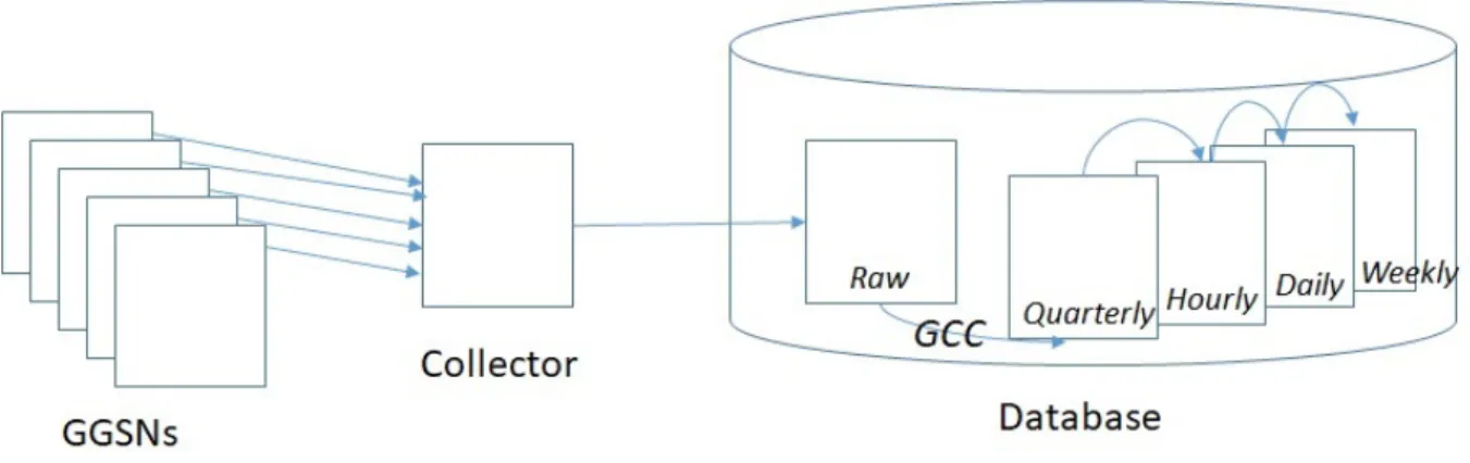
this study. Figure 2.1gives an overview of what is covered. This investigation was required
to understand the content of the data as well to as identify potential data corruption and data completeness issues which themselves can be presented as anomalies.
The source of the data are the GGSN/SGW/PGW nodes in the mobile network. Each node has been configured to measure and record the activities it is involved in. This data is saved locally to a file referred to as a “Bulkstats” file. Each node generates a new “Bulkstats” file every 15 minutes to capture the data associated with that 15 minute interval. Each file is divided up into groups of counters referred to as schema. There is one schema for each major function performed by each node. For example the “RADIUS” schema holds all the counters associated with the RADIUS function while the “Diameter” Schema holds counters associated with the Diameter function.
Each schema holds two types of data. The first are referred to as the “Statistics” and the
second are referred to as the “Key Variables” [19]. The statistics can be one of three types.
The first is of type “counter”, which increments with each event counted, until the counter limit is reached and the counter rolls-over back to zero. An example of this would be the count of the number of bytes going through an interface. The second is of type “Gauge”, which gives an absolute value at a point in time. An example of this is the number of data session supported at one point in time. The last type is “information” which is used to differentiate sets of statistics. An example of this would be an IP address. The second type of data held in a schema are the “key variables”. These identify the dimensions that
the “Statistics” are associated with and vary from schema to schema. Table 2.1 on page
15 lists the number of “statistics” and “key variables” associated with each schema.
Both the “Statistics” and “Key Variables” are stored in one of 4 data types. These are int32, which is a 32 bit integer, which rolls over at 4,294,967,295, Int64 which rolls over at 18,446,744,073,709,551,615, Float, which include decimal points and lastly String, which is used to represent characters.
Figure 2.1: Flow of data from Generation through GCC and Aggregation to Storage.
“Bulkstats” files from the GGSN/SGW/PGW nodes and passes them on to the the database function. The Database function loads the data into “Raw” tables, joining all the schema from the individual nodes together. This results in there being a table or
a set of tables per schema. Table 2.1 on page 15lists the 26 schema.
As part of the loading process, the GGSN/SGW/PGW ID, the geographical region that the node is located in and the start time of the 15 min interval are added to each line of the table or tables. The data base function creates a “QTR” table associated with each “RAW” table by gauge counter correcting (GCC) the statistics of type “Counter”. This process involves subtracting the counter value of the previous interval from the current interval to obtain the absolute value associated with that 15 minute period. The “statistics” of type “Gauge” are copied directly from the “Raw” tables to the “QTR” tables . The Database function is then responsible for aggregating data up in the time domain to hourly, daily, weekly, monthly and yearly tables. The database function is lastly responsible for deleting old data. The retention periods for each table type is given
in table Table 2.2.
An investigation of the data flow reveals that there are several anomalies that arise in the data as a result of issues in processing of the data. These anomalies are described below, starting with the generation of the data on the GGSN/SGW/PGW nodes and ending with the aggregation of the data in the time domain. When generating the “statistics” of type “counter”, it is expected that the counter value will roll over back to zero when it exceeds the maximum value that can be represented by the data types described above. Two scenarios have been identified where this is not the case. The first case presents itself when the process responsible for managing the counters restarts. When this happens all the counter increments for the associated 15 minute interval are reset. This results in counters being reset more frequently. This varies in frequency between the nodes. The nodes carrying more traffic have higher number of occurrences. The second case where the roll over occurs too frequently are in the cases where the data type used for the counter
is not large enough to represent the increase in the statistic. Figure 2.2 on page16shows
an example of the happening with counter G25M0C2. Sub-figure a shows the values for GGCT03 as a monotonically increasing function in the raw stats for all data points except for the first 3 which have experienced a roll over. Sub-figure b shows how the raw data is gauge counter corrected (GCC), effectively showing the counter values for GGCT03 (except for the first 3 data points). GGPS02 however carries more traffic, resulting in the counter rolling over in every 15 minute interval. Sub-figure b shows the corrupted for GGPS02 data after GCC.
The next group of potential anomalies are introduced by the ETL process. Occurrences were observed where the collector function is interrupted. This results in missing data on
Table 2.1: Data “statistics” and “key variable” counts.
Schema Tables Sub Schema Key Variables Statistics
APN 4 4 3 309 APNQCI 1 1 2 16 CARD 3 3 1 136 DCCA 2 2 4 26 DCCASCH 1 3 2 123 DIAUSCH 1 1 7 44 DISCH 1 1 1 53 DPCA 3 4 4 41 ECS 12 12 0 1669 EGTPC 6 9 4 564 GTPC 5 5 6 276 GTPP 3 3 2 180 GTPU 2 2 4 91 IMSA 2 2 4 165 IPPOOL 1 1 8 13 LINK 1 5 2 180 P2PSCH 1 1 7 5 PDSN 15 22 7 2754 PES2A 2 25 5 488 PES2B 2 27 5 568 PES5S81 3 50 5 965 PGW 10 11 4 553 PORT 1 1 2 32 RADIUSGRP 1 1 7 78 RULEBASE 1 1 1 6 SGW 16 19 4 994
Table 2.2: Data retention periods.
Table type Retention period
RAW 14 days 15 minutes 14 days Hourly 90 days Daily 400 days Weekly 2 years Monthly 5 years Yearly 10 years
● ● ● ● ● ● ● ● ● ● ● ● ●● ● ● ● ● ● ● ● ● ●●● ● ● ● ● ● ● ● ● ● ● ● ● ● ● ● ● ● ● ● ● ● ● ● ● ● ●● ● ● ● ● ● ● ● ● ● ● ● ● ● ● ● ● ● ● ● ● ● ● ●● ● ● ● ● ●● ● ● ● ● ● ● ● ● ● ● ● ●● ● ● ● ● ● ● ● ● ● ● ● ● ● ● ● ● ● ● ● ● ● ● ● ● ● ● ● ● ● ● ● ● ● ● ● ● ● ● ● ● ● ● ● ● ● ● ● ● ●● ● ● ● ● ● ● ● ● ● ● ● ● ● ● ● ● ● ● ● ● ● ● ● ●● ● ● ● ● ● ● ● ● ● ● ● ● ● ● ● ● ● ● 0e+00 1e+09 2e+09 3e+09 4e+09
Feb 23 12:00 Feb 23 18:00 Feb 24 00:00 Feb 24 06:00 Feb 24 12:00 STARTTIME G25M0C2 ELEMENT_ID ● ● GGCT03 GGPS02
(a) Raw data.
● ● ● ●● ●● ● ● ● ●● ● ● ● ● ● ●●●●●● ● ● ● ● ● ● ● ● ●● ● ● ● ● ● ●● ● ● ● ● ● ● ● ● ● ● ● ● ● ●● ● ● ●● ● ● ● ● ●●● ● ● ● ● ● ● ● ● ●● ● ● ● ● ● ● ● ● ● ● ● ● ● ● ● ● ● ● ● ● ● ● ● ● ● ● ● ● ● ● ● ● ● ● ● ● ● ● ●● ● ● ● ● ● ● ● ● ● ● ● ● ● ● ● ●● ● ● ● ● ● ● ● ● ● ● ● ● 0e+00 1e+09 2e+09 3e+09
Feb 23 12:00 Feb 23 18:00 Feb 24 00:00 Feb 24 06:00 STARTTIME G25M0C2 ELEMENT_ID ● ● GGCT03 GGPS02
(b) Gauge counter corrected data. Figure 2.2: Raw data showing roll overs on counter G25M0C2.
all or some of the nodes. A miss-alignment in the timing between the collector and the database results in examples where the statistics are double counted or missing for a subset of the nodes. Incorrect “statistics” definitions on the database function results in data being corrupted during the creation of the QTR table. Instances were found where some statistics of type “Gauge” were treated as type “Counter” and some of type “Counter” were treated as type “Gauge”. Lastly some counters had the incorrect aggregation rule applied to them for the time domain aggregations. For example a counter measuring a percentage should be aggregated using a maximum or average function and not a sum function, and likewise a counter measuring the count of packets, should be aggregated using sum and not average or maximum.
With the goal of reducing the impact of data corruption on the subsequent anomaly detection methods the following steps were taken. The counter type definitions were audited and corrected. The timers controlling the database loading from the collectors were adjusted to ensure no missing or duplicated stats. The use of the incorrect data types resulting in roll overs were logged with the equipment vendor (the fixes for these would only be made available in the following software release). The aim was to address the rest of the anomalies introduced in the data flow through filtering them out. This meant that the QTR tables would have to form the basis of the study as the tables with the higher time domain aggregation had already aggregated the missing and corrupted data in with clean data.
The study focuses on the data contained in the SGW Schema.
2.2
SGW Data Description
The SGW schema contains 994 “statistics”, four Key Variables and the added start time and SGW element dimensions. The data sample extracted was for a 14 day interval from 2018-02-24 09h00 to 2018-03-10 08h15 and consisted of 28161 observations. The key
variables include The VPN id, VPN NAME, SERV ID and SERV NAME. Table 2.3 on
page 17 shows the break down of these per GGSN/PGW/SGW node. Each node only
has one VPN ID and one SERV ID and which map to the VPN NAME of “SGW” and SERV NAME of “SGW SVC” respectively. The key variables therefore do not indicate any sub dimension and can be ignored.
Table 2.3: SGW Schema Key variables.
SGW ID VPN ID VPN NAME SERV ID SERV NAME
CSGNMT01 6 SGW 8 SGW SVC GGCF01 4 SGW 9 SGW SVC GGCF02 5 SGW 9 SGW SVC GGCT01 14 SGW 9 SGW SVC GGCT03 7 SGW 9 SGW SVC GGCT04 7 SGW 9 SGW SVC GGDM01 4 SGW 9 SGW SVC GGDM02 3 SGW 3 SGW SVC GGDN01 9 SGW 9 SGW SVC GGDN02 9 SGW 9 SGW SVC GGDN03 3 SGW 3 SGW SVC GGJF01 4 SGW 9 SGW SVC GGMT01 20 SGW 11 SGW SVC GGMT03 7 SGW 9 SGW SVC GGMT04 7 SGW 9 SGW SVC GGPR01 4 SGW 9 SGW SVC GGPS02 18 SGW 9 SGW SVC GGPS03 7 SGW 9 SGW SVC GGPS04 5 SGW 3 SGW SVC NFV1-GGMD01 5 SGW 9 SGW SVC NFV1-GGPR02 3 SGW 9 SGW SVC
The SGW nodes are deployed across 4 regions as shown in Table 2.4
Table 2.4: Regional location of GGSN/PGW/SGW nodes.
CTN DBN JHB PTA GGCF01 GGDM01 GGJF01 GGPR01 GGCF02 GGDM02 GGMT01 GGPS02 GGCT01 GGDN01 GGMT03 GGPS03 GGCT03 GGDN02 GGMT04 GGPS04 GGCT04 GGDN03 NFV1-GGPR02 NFV1-GGMD01
The software program R [20] was used for all subsequent data analysis and model building.
The following processes was used to clean the SGW data. The variables consisting on only zero values were removed first. The variables with a high percentage of N/A entries
were then removed. Next, the observations with an N/A entry were removed. The
threshold used for the percentage of N/As per variable, affected how many observations were removed in the final step. This threshold was selected to minimize the amount of data removed from the original data set. Lastly it was observed that some of the nodes did not support the SGW function. The observations for these nodes only contained zeros and were removed.
Out of the original 994 variables, 636 contained only zeros, leaving 358. The remaining
variables consisted of only positive integers and N/A. TableTable 2.5on page18shows the
Table 2.5: Variables count per N/A number.
Variable Count N/A Count
670 0 6 1 17 2 28 3 11 4 28 5 2 6 5 7 24 8 93 9 104 10 3 11 1 81 1 137 1 139 1 584 1 8075 1 8997
variables with 0 N/A present and there was 1 variable with 8997 observations containing N/A. All variables containing more than 11 N/A were removed from the data set. This left 349 of the original 994 variables. After removing observations containing N/A 28148 of the original 28161 observations remained. 9 of the nodes didn’t support the SGW function were removed, leaving 12 nodes. The observations remaining after the removal
of these nodes was 16070. Table 2.6 on page 18 shows that in the final SGW data set,
the number of observations per nodes is balanced.
Table 2.6: Observations per GGSN/SGW/PGW in the final SGW Data.
SGW ID Observations GGCF01 1342 GGCT03 1342 GGCT04 1342 GGDM01 1337 GGDN01 1342 GGDN02 1337 GGJF01 1341 GGMT03 1342 GGMT04 1332 GGPR01 1336
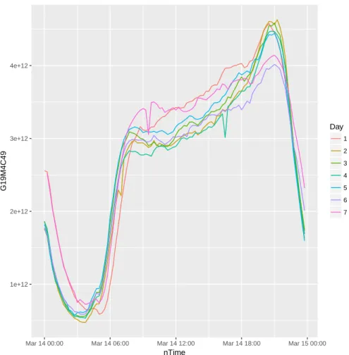
The activity supported by the SGW function is expected to be periodic, following the activity of the mobile subscribers. Variable G19M4C49 represents the down link bytes on
the S1U interface of the SGW. Figure 2.3, Figure 2.4 and Figure 2.5 show the following
characteristics of the data volumes supported by the SGWs.
0e+00 2e+11 4e+11 6e+11 8e+11
Feb 28 Mar 01 Mar 02 Mar 03
Date.Time G19M4C49 SGW_ID GGCF01 GGCT03 GGCT04 GGDM01 GGDN01 GGDN02 GGJF01 GGMT03 GGMT04 GGPR01 GGPS03 GGPS04
Figure 2.3: S1U Down link Bytes per SGW.
hours of the morning and the highest being at 21h00
• The traffic volumes supported by the different SGW nodes varies with GGPS04
carrying the most traffic and GGDM01 the least
• The traffic volumes on the first of the month are higher than the traffic on the last
day of the month
• The traffic volumes on a Saturday and a Sunday stays higher into the early hours
of the morning compared to a weekday
• The traffic volumes on a Sunday stays lower for longer in the morning than the
other 6 days of the week
• The difference in traffic volumes between the mid-morning and late evening in lowest
on a Saturday.
There are two dips seen on the day 7 and day 4 of Figure 2.3. These caused by there
being a missing observation for GGMT04.
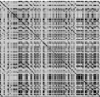
As the variables are measurements of the various activities supported by the node, it is expected that there will be high levels of correlation between the variables. For example, in the early hours of the morning, when the majority of subscribers are sleeping, very few subscribers will be sending or receiving data, this means that the number of packets sent, bytes send, packets received, bytes received, will be lower for all 9 Quality of Service Class Indicator groups. This means that all 36 counters measuring these will have low values. As people start waking up and using data all of these counters will start increasing in
1e+12 2e+12 3e+12 4e+12
Mar 14 00:00 Mar 14 06:00 Mar 14 12:00 Mar 14 18:00 Mar 15 00:00
nTime G19M4C49 Day 1 2 3 4 5 6 7
Figure 2.4: Day of week comparison.
sync. As there are too many variables to show in a correlation matrix, the correlation matrix is represented in a bitmap format where correlations of 1 are shown as black and
-1 as white. Everything in between is shown as in varying shades of gray. Figure 2.6
shows the high levels of correlation.
Figure 2.7 and Figure 2.8 show a summary of the SGW variables. There is not an even distribution of the values, with one grouping of low values dominating the results. A log scale on the x axis is used to show the distribution more clearly.
2.3
Methods
The approach taken is to prepare the data set so that it can ultimately be used in a semi-supervised learning approach. This required the identification and removal of outliers from the original raw data. To achieve this, Principal Component Analysis (PCA) is first used to reduce the number of variables. This data is then presented to 4 anomaly detection techniques, namely K-nearest neighbours, One Class Support Vector Machines, Density-Based Local Outlier Factor and Multivariate Gaussian Distributions. The results are used to identify and remove the observations most likely to be anomalies within the raw data set. The resulting data set forms the input to a semi-supervised learning approach.
2.3.1
Dimensionality Reduction
As shown inFigure 2.6, the SGW data is highly correlated and will therefore benefit from
1e+12 2e+12 3e+12 4e+12
Mar 04 Mar 06 Mar 08 Mar 10
Date.Time
G19M4C49
Figure 2.5: Total network S1U bytes down over 7 days.
0 10 20 30 40 50
1e−02 1e+02 1e+06 1e+10
value
count
(a) Histogram of the means of the SGW variables.
0 10 20 30 40
1e+02 1e+05 1e+08 1e+11
value
count
(b) Histogram of the maxes of the SGW variables.
0 10 20 30
1e+02 1e+05 1e+08 1e+11
value
count
(c) Histogram of the medians of the SGW variables. Figure 2.7: SGW data summary.
0 10 20 30 40
1e+00 1e+04 1e+08
value
count
(a) Histogram of the standard deviation of the SGW variables.
0 10 20 30 40
1e+00 1e+07 1e+14 1e+21
value
count
(b) Histogram of the variances of the SGW variables. Figure 2.8: SGW data summary.
Figure 2.9: Cumulative Variation explained by all 349 principal components.
removes redundancy in the data by creating new independent variables (principal components) that are linear combinations of the original variables. The first principal component explains the most variation in the data, with each subsequent principal component explaining less and less. The goal is to reduce the number of dimensions/ variables used in the subsequent anomaly detection techniques employed to remove anomalies from the data as preparation for the semi-supervised learning approach. Added to this the impact of the “curse of dimensionality” will be reduced in the subsequent analysis.
The variation explained by the first 3 principal components of the SGW data is 8.55%,
5.52% and 3.12% respectively, making up 17.2% together. The first 60 principal
components explain 81.67% of the variation and the first 100 are needed to explain
95.23%. Figure 2.9 on page 24 shows the cumulative variation explained by all 349
principal components.
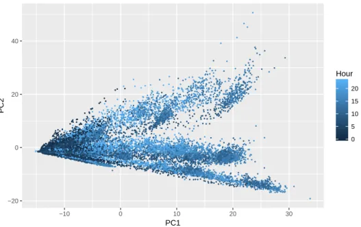
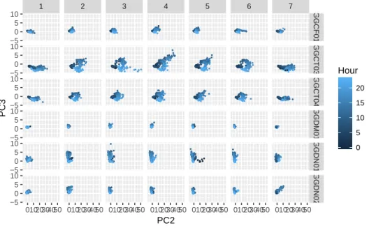
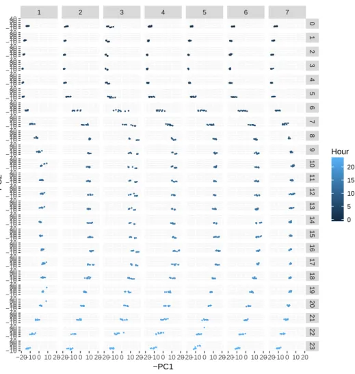
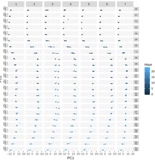
The plot of the first two principal components in Figure 2.10 shows potential clusters
based on the time of day with observations occurring at the same time of day being
grouped together. Figure 2.11 shows that the observations generated by each node also
form clusters. ● ● ● ● ● ● ● ● ● ● ● ● ● ● ● ● ● ● ● ● ● ● ● ● ● ● ● ● ● ● ● ● ● ● ● ● ● ● ● ● ● ● ● ●● ● ● ● ● ● ● ● ● ● ● ● ● ● ● ● ● ● ● ● ● ● ● ● ● ● ● ● ● ● ● ● ● ● ● ● ● ● ● ● ● ● ● ● ● ● ● ●● ● ● ● ● ● ● ● ● ● ● ● ● ● ● ● ● ● ● ● ● ● ● ● ● ● ● ● ● ● ● ● ● ● ● ● ● ● ● ● ● ● ● ● ● ● ● ● ● ● ● ● ● ● ● ● ● ● ● ● ● ● ● ● ● ● ● ● ● ● ● ● ● ● ● ● ● ● ● ● ● ● ● ● ● ● ● ● ● ● ● ● ● ● ● ●● ● ● ● ● ● ● ● ● ● ● ● ● ● ● ● ● ● ● ● ● ● ● ● ● ● ● ● ● ● ● ● ● ● ● ●● ● ● ● ● ● ● ● ● ● ● ● ● ● ● ● ● ● ● ● ● ● ● ●● ● ● ● ● ● ● ● ● ● ● ● ● ● ● ● ● ● ● ● ● ● ● ● ● ● ● ● ● ● ● ● ● ● ● ●● ● ● ● ● ● ● ● ● ● ● ● ● ● ● ● ● ● ● ● ● ● ● ● ● ● ● ● ● ● ● ● ● ● ● ● ● ● ● ● ● ● ● ● ● ● ● ● ● ● ● ● ● ● ● ● ● ● ● ● ● ● ● ● ● ● ● ● ● ● ● ● ● ● ● ● ● ● ● ● ● ● ● ●● ● ● ● ● ● ● ● ● ● ● ● ● ● ● ● ● ● ● ● ● ● ● ● ● ● ● ● ● ● ● ● ● ● ● ● ● ● ● ● ● ● ● ● ● ● ● ●● ● ● ● ● ● ● ● ● ● ● ●● ● ● ● ● ● ● ● ● ● ● ● ● ● ● ● ● ● ● ● ● ● ● ●● ● ● ● ● ● ● ● ● ● ● ● ● ● ● ● ● ● ● ● ● ● ● ● ● ● ● ● ● ● ● ● ● ● ● ●● ● ● ● ● ● ● ● ● ● ● ● ● ● ● ● ● ● ● ● ● ● ● ●● ● ● ● ● ● ● ● ● ● ● ● ● ● ● ● ● ● ● ● ● ● ● ● ● ● ● ● ● ● ● ● ● ● ● ● ● ● ● ● ● ● ● ● ● ● ● ● ● ● ● ● ● ● ● ● ● ● ● ● ● ● ● ● ● ● ● ● ● ● ● ● ● ● ● ● ● ● ● ● ● ● ● ● ● ● ● ● ● ● ● ● ● ● ● ●● ● ● ● ● ● ● ● ● ● ● ● ● ● ● ● ● ● ● ● ● ● ● ● ● ● ● ● ● ● ● ● ● ● ● ● ● ● ● ● ● ● ● ● ● ● ● ●● ● ● ● ● ● ● ● ● ● ● ● ● ● ● ● ● ● ● ● ● ● ● ● ● ● ● ● ● ● ● ● ● ● ● ● ● ● ● ● ● ● ● ● ● ● ● ● ● ● ● ● ● ● ● ● ● ● ● ● ● ● ● ● ● ● ● ● ● ● ● ●● ● ● ● ● ● ● ● ● ● ● ● ● ● ● ● ● ● ● ● ● ● ● ●● ● ● ● ● ● ● ● ● ● ● ● ● ● ● ● ● ● ● ● ● ● ● ● ● ● ● ● ● ● ● ● ● ● ● ● ● ● ● ● ● ● ● ● ● ● ● ●● ● ● ● ● ● ● ● ● ● ● ● ● ● ● ● ● ● ● ● ● ● ● ● ● ● ● ● ● ● ● ● ● ● ● ●● ● ● ● ● ● ● ● ● ● ● ● ● ● ● ● ● ● ● ● ● ● ● ●● ● ● ● ● ● ● ●● ● ● ●● ● ● ● ● ● ● ● ● ● ● ●● ● ● ● ● ● ● ● ● ● ● ●● ● ● ● ● ● ● ● ● ● ● ●● ● ● ● ● ● ● ● ● ● ● ●● ● ● ● ● ● ● ● ● ● ● ● ● ● ● ● ● ● ● ● ● ● ● ●● ● ● ● ● ● ● ● ● ● ● ●● ● ● ● ● ● ● ● ● ● ● ●● ● ● ● ● ● ● ● ● ● ● ● ● ● ● ● ● ● ● ● ● ● ● ●● ● ● ● ● ● ● ● ● ● ● ● ● ● ● ● ● ● ● ● ● ● ● ●● ● ● ● ● ● ● ● ● ● ● ●● ● ● ● ● ● ● ● ● ● ● ● ● ● ● ● ● ● ● ● ● ● ● ● ● ● ● ● ● ● ● ● ● ● ● ● ● ● ● ● ● ● ● ● ● ● ● ●● ● ● ● ● ● ● ● ● ● ● ●● ● ● ● ● ● ● ● ● ● ● ● ● ● ● ● ● ● ● ● ● ● ● ● ● ● ● ● ● ● ● ● ● ● ● ● ● ● ● ● ● ● ● ● ● ● ● ● ● ● ● ● ● ● ● ● ● ● ● ● ● ● ● ● ● ● ● ● ● ● ● ●● ● ● ● ● ● ● ● ● ● ● ● ● ● ● ● ● ● ● ● ● ● ● ●● ● ● ● ● ● ● ● ● ● ● ● ● ● ● ● ● ● ● ● ● ● ● ● ● ● ● ● ● ● ● ● ● ● ● ● ● ● ● ● ● ● ● ● ● ● ● ● ● ● ● ● ● ● ● ● ● ● ● ● ● ● ● ● ● ● ● ● ● ● ● ● ● ● ● ● ● ● ● ● ● ● ● ● ● ● ● ● ● ● ● ● ● ● ● ● ● ● ● ● ● ● ● ● ● ● ● ● ● ● ● ● ● ● ● ● ● ● ● ● ● ● ● ● ● ● ● ● ● ● ● ● ● ● ● ● ● ● ● ● ● ● ● ●● ● ● ● ● ● ● ● ● ● ● ●● ● ● ● ● ● ● ● ● ● ● ● ● ● ● ● ● ● ● ● ● ● ● ● ● ● ● ● ● ● ● ● ● ● ● ● ● ● ● ● ● ● ● ● ● ● ● ● ● ● ● ● ● ● ● ● ● ● ● ● ● ● ● ● ● ● ● ● ● ● ● ●● ● ● ● ● ● ● ● ● ● ● ● ● ● ● ● ● ● ● ● ● ● ● ● ● ● ● ● ● ● ● ● ● ● ● ● ● ● ● ● ● ● ● ● ● ● ● ● ● ● ● ● ● ● ● ● ● ● ●● ● ● ● ● ● ● ● ● ● ● ● ● ● ● ● ● ● ● ● ● ● ● ● ● ● ● ● ● ● ● ● ● ● ● ● ● ● ● ● ● ● ● ● ● ● ● ● ● ● ● ● ● ● ● ● ● ● ● ● ● ● ● ● ● ● ● ● ● ● ● ● ● ● ● ● ● ● ● ● ● ● ● ● ● ● ● ● ● ● ● ● ● ● ● ●● ● ● ● ● ● ● ● ● ● ● ● ● ● ● ● ● ● ● ● ● ● ● ● ● ● ● ● ● ● ● ● ● ● ● ● ● ● ● ● ● ● ● ● ● ● ● ● ● ● ● ● ● ● ● ● ● ● ● ● ● ● ● ● ● ● ● ● ● ● ● ● ● ● ● ● ● ● ● ● ● ● ● ● ● ● ● ● ● ● ● ● ● ● ● ● ● ● ● ● ● ● ● ● ● ● ● ● ● ● ● ● ● ● ● ● ● ● ● ● ● ● ● ● ● ● ● ● ● ● ● ● ● ● ● ● ● ● ● ● ● ● ● ● ● ● ● ● ● ● ● ● ● ● ● ● ● ● ● ● ● ● ● ● ● ● ● ● ● ● ● ● ● ● ● ● ● ● ● ● ● ● ● ● ● ● ● ● ● ● ● ● ● ● ● ● ● ● ● ● ● ● ● ● ● ● ● ● ● ● ● ● ● ● ● ●● ● ● ● ● ● ● ● ● ● ● ● ● ● ● ● ● ● ● ● ● ● ● ● ● ● ● ● ● ● ● ● ● ● ● ●● ● ● ● ● ● ● ● ● ● ● ● ● ● ● ● ● ● ● ● ● ● ● ● ● ● ● ● ● ● ● ● ● ● ● ●● ● ● ● ● ● ● ● ● ● ● ● ● ● ● ● ● ● ● ● ● ● ● ● ● ● ● ● ● ● ● ● ● ● ● ● ● ● ● ● ● ● ● ● ● ● ● ●● ● ● ● ● ● ● ● ● ● ● ●● ● ● ● ● ● ● ● ● ● ● ● ● ● ● ● ● ● ● ● ● ● ● ●● ● ● ● ● ● ● ● ●● ● ● ● ● ● ● ● ● ● ● ● ● ● ● ● ● ● ● ● ● ● ● ● ● ● ● ● ● ● ● ● ● ● ● ● ● ● ●● ● ● ● ● ● ● ● ● ●● ●●●● ● ● ● ● ● ● ● ● ●● ● ● ● ● ● ● ● ● ● ● ● ● ● ● ● ● ● ● ● ● ●● ●●●● ● ● ● ● ● ● ● ● ● ● ● ● ● ● ● ● ● ● ● ● ● ● ● ● ● ● ● ● ●●● ● ●● ● ● ● ● ● ● ●●● ● ●● ● ● ● ● ● ● ● ● ● ● ● ● ● ● ● ● ● ● ● ● ● ● ●● ● ● ● ● ● ● ● ● ● ● ●● ● ● ● ● ● ● ● ● ● ● ●● ● ● ● ● ● ● ● ● ● ● ● ● ● ● ● ● ● ● ● ● ● ● ●● ● ● ● ● ● ● ● ● ● ● ●● ● ● ● ● ● ● ● ● ● ● ● ● ● ● ● ● ● ● ● ● ● ● ● ● ● ● ● ● ● ● ● ● ● ● ●● ● ● ● ● ● ● ● ● ● ● ● ● ● ● ● ● ● ● ● ● ● ● ● ● ● ● ● ● ● ● ● ● ● ● ● ● ● ● ● ● ● ● ● ● ● ● ● ● ● ● ● ● ● ● ● ● ● ● ● ● ● ● ● ● ● ● ● ● ● ● ● ● ● ● ● ● ● ● ● ● ● ● ● ● ● ● ● ● ● ● ● ● ● ● ● ● ● ● ● ● ● ● ● ● ● ● ● ● ● ● ● ● ● ● ● ● ● ● ● ● ● ● ● ● ● ● ● ● ● ● ● ● ● ● ● ● ● ● ● ● ● ● ● ● ● ● ● ● ● ● ● ● ● ● ● ● ● ● ● ● ● ● ● ● ● ● ● ● ● ● ● ● ● ● ● ● ● ● ● ● ● ● ● ● ● ● ● ● ● ● ● ● ● ● ● ● ● ● ● ● ● ● ● ● ● ● ● ● ● ● ● ● ● ● ● ● ● ● ● ● ● ● ● ● ● ● ● ● ● ● ● ● ● ● ● ● ● ● ● ● ● ● ● ● ● ● ● ● ● ● ● ● ● ● ● ● ● ● ● ● ● ● ● ● ● ● ● ● ● ● ● ● ● ● ● ● ● ● ● ● ● ● ● ● ● ● ● ● ● ● ● ● ● ● ● ● ● ● ● ● ● ● ● ● ● ● ● ● ● ● ● ● ● ● ● ● ● ● ● ● ● ● ●● ● ● ● ● ● ● ● ● ● ● ● ● ● ● ● ● ● ● ● ● ● ● ● ● ● ● ● ● ● ● ● ● ● ● ● ● ● ● ● ● ● ● ● ● ● ● ● ● ● ● ● ● ● ● ● ● ● ● ● ● ● ● ● ● ● ● ● ● ● ● ●● ● ● ● ● ● ● ● ● ● ● ●● ● ● ● ● ● ● ● ● ● ● ●● ● ● ● ● ● ● ● ● ● ● ● ● ● ● ● ● ● ● ● ● ● ● ● ● ● ● ● ● ● ● ● ● ● ● ● ● ● ● ● ● ● ● ● ● ● ● ● ● ● ● ● ● ● ● ● ● ● ● ● ● ● ● ● ● ● ● ● ● ● ● ●● ● ● ● ● ● ● ● ● ● ● ● ● ● ● ● ● ● ● ● ● ● ● ● ● ● ● ● ● ● ● ● ● ● ● ● ● ● ● ● ● ● ● ● ● ● ● ● ● ● ● ● ● ● ● ● ● ● ● ● ● ● ● ● ● ● ● ● ● ● ● ●● ● ● ● ● ● ● ● ● ● ● ● ● ● ● ● ● ● ● ● ● ● ● ● ● ● ● ● ● ● ● ● ● ● ● ●● ● ● ● ● ● ● ● ● ● ● ● ● ● ● ● ● ● ● ● ● ● ● ●● ● ● ● ● ● ● ● ● ● ● ● ● ● ● ● ● ● ● ● ● ● ● ● ● ● ● ● ● ● ● ● ● ● ● ● ● ● ● ● ● ● ● ● ● ● ● ● ● ● ● ● ● ● ● ● ● ● ● ●● ● ● ● ● ● ● ● ● ● ● ● ● ● ● ● ● ● ● ● ● ● ● ●● ● ● ● ● ● ● ● ● ● ● ● ● ● ● ● ● ● ● ● ● ● ● ● ● ● ● ● ● ● ● ● ● ● ● ● ● ● ● ● ● ● ● ● ● ● ● ●● ● ● ● ● ● ● ● ● ● ● ● ● ● ● ● ● ● ● ● ● ● ● ● ● ● ● ● ● ● ● ● ● ● ● ● ● ● ● ● ● ● ● ● ● ● ● ● ● ● ● ● ● ● ● ● ● ● ● ● ● ● ● ● ● ● ● ● ● ● ● ● ● ● ● ● ● ● ● ● ● ● ● ● ● ● ● ● ● ● ● ● ● ● ● ● ● ● ● ● ● ● ● ● ● ● ● ● ● ● ● ● ● ● ● ● ● ● ● ● ● ● ● ● ● ● ● ● ● ● ● ● ● ● ● ● ● ● ● ● ● ● ● ● ● ● ● ● ● ● ● ● ● ● ● ● ● ● ● ● ● ● ● ● ● ● ● ● ● ● ● ● ● ● ● ● ● ● ● ● ● ● ● ● ● ● ● ● ●● ● ● ● ● ● ● ● ● ● ● ● ● ● ● ● ● ● ● ● ● ● ● ● ● ● ● ● ● ● ● ● ● ● ● ● ● ● ● ● ● ● ● ● ● ● ● ● ● ● ● ● ● ● ● ● ● ● ● ● ● ● ● ● ● ● ● ● ● ● ● ● ● ● ● ● ● ● ● ● ● ● ● ● ● ● ● ● ● ● ● ● ● ● ● ● ● ● ● ● ● ● ● ● ● ● ● ● ● ● ● ● ● ● ● ● ● ● ● ● ● ● ● ● ● ● ● ● ● ● ● ● ● ● ●● ● ● ● ● ● ● ● ● ● ● ●● ● ● ● ● ● ● ● ● ● ● ●● ● ● ● ● ● ● ● ● ● ● ● ● ● ● ● ● ● ● ● ● ● ● ● ● ● ● ● ● ● ● ● ● ● ● ● ● ● ● ● ● ● ● ● ● ● ● ● ● ● ● ● ● ● ● ● ● ● ● ●● ● ● ● ● ● ● ● ● ● ● ● ● ● ● ● ● ● ● ● ● ● ● ● ● ● ● ● ● ● ● ● ● ● ● ● ● ● ● ● ● ● ● ● ● ● ● ● ● ● ● ● ● ● ● ● ● ● ● ● ● ● ● ● ● ● ● ● ● ● ● ● ● ● ● ● ● ● ● ● ● ● ● ● ● ● ● ● ● ● ● ● ● ● ● ● ● ● ● ● ● ● ● ● ● ● ● ● ● ● ● ● ● ● ● ● ● ● ● ●● ● ● ● ● ● ● ● ● ● ● ● ● ● ● ● ● ● ● ● ● ● ● ● ● ● ● ● ● ● ● ● ● ● ● ● ● ● ● ● ● ● ● ● ● ● ● ● ● ● ● ● ● ● ● ● ● ● ● ● ● ● ● ● ● ● ● ● ● ● ● ●● ● ● ● ● ● ● ● ● ● ● ●● ● ● ● ● ● ● ● ● ● ● ● ● ● ● ● ● ● ● ● ● ● ● ● ● ● ● ● ● ● ● ● ● ● ● ● ● ● ● ● ● ● ● ● ● ● ● ●● ● ● ● ● ● ● ● ● ● ● ● ● ● ● ● ● ● ● ● ● ● ● ● ● ● ● ● ● ● ● ● ● ● ● ● ● ● ● ● ● ● ● ● ● ● ● ● ● ● ● ● ● ● ● ● ● ● ● ● ● ● ● ● ● ● ● ● ● ● ● ● ● ● ● ● ● ● ● ● ● ● ● ● ● ● ● ● ● ● ● ● ● ● ● ● ● ● ● ● ● ● ● ● ● ● ● ● ● ● ● ● ● ● ● ● ● ● ● ●● ● ● ● ● ● ● ● ● ● ● ●● ● ● ● ● ● ● ● ● ● ● ● ● ● ● ● ● ● ● ● ● ● ● ●● ● ● ● ● ● ● ● ● ● ● ● ● ● ● ● ● ● ● ● ● ● ● ● ● ● ● ● ● ● ● ● ● ● ● ● ● ● ● ● ● ● ● ● ● ● ● ● ● ● ● ● ● ● ● ● ● ● ● ●● ● ● ● ● ● ● ● ● ● ● ● ● ● ● ● ● ● ● ● ● ● ● ● ● ● ● ● ● ● ● ● ● ● ● ● ● ● ● ● ● ● ● ● ● ● ● ● ● ● ● ● ● ● ● ● ● ● ● ●● ● ● ● ● ● ● ● ● ● ● ●● ● ● ● ● ● ● ● ● ● ● ● ● ● ● ● ● ● ● ● ● ● ● ●● ● ● ● ● ● ● ● ● ● ● ●● ● ● ● ● ● ● ● ● ● ● ● ● ● ● ● ● ● ● ● ● ● ● ●● ● ● ● ● ● ● ● ● ● ● ● ● ● ● ● ● ● ● ● ● ● ● ● ● ● ● ● ● ● ● ● ● ● ● ●● ● ● ● ● ● ● ● ● ● ● ● ● ● ● ● ● ● ● ● ● ● ● ●● ● ● ● ● ● ● ● ● ● ● ● ● ● ● ● ● ● ● ● ● ● ● ● ● ● ● ● ● ● ● ● ● ● ● ● ● ● ● ● ● ● ● ● ● ● ● ● ● ● ● ● ● ● ● ● ● ● ● ● ● ● ● ● ● ● ● ● ● ● ● ● ● ● ● ● ● ● ● ● ● ● ● ● ● ● ● ● ● ● ● ● ● ● ● ● ● ● ● ● ● ● ● ● ● ● ● ● ● ● ● ● ● ● ● ● ● ● ● ● ● ● ● ● ● ● ● ● ● ● ● ● ● ● ● ● ● ● ● ● ● ● ● ● ● ● ● ● ● ● ● ● ●● ● ● ● ● ● ● ● ● ● ● ● ● ● ● ● ● ● ● ● ● ● ● ● ● ● ●● ● ● ● ● ● ● ● ● ● ● ● ● ● ● ● ● ● ● ● ● ● ● ● ● ● ● ● ● ● ● ● ● ● ● ● ● ● ● ● ● ● ● ● ● ● ● ●● ● ● ● ● ● ● ● ● ● ● ●● ● ● ● ● ● ● ● ● ● ● ●● ● ● ● ● ● ● ● ●● ● ● ● ● ● ● ● ● ● ● ● ● ● ● ● ● ● ● ● ● ● ● ●● ● ● ● ● ● ● ● ● ● ● ● ● ● ●● ● ● ● ● ● ● ● ● ● ● ● ● ● ● ● ● ● ● ● ● ● ● ●● ● ● ● ● ● ● ● ● ● ● ● ● ● ● ● ● ● ● ●●● ● ●● ● ● ● ● ● ● ● ●● ● ●● ● ● ● ● ● ● ● ●● ● ●● ● ● ● ● ● ● ● ● ● ●●● ● ● ● ● ● ● ● ● ● ● ●● ● ● ● ● ● ● ● ● ● ● ● ● ● ● ● ● ● ● ● ● ● ● ● ● ● ● ● ● ● ● ● ● ● ● ● ● ● ● ● ● ● ● ● ● ● ● ● ● ● ● ● ● ● ● ● ● ● ● ● ● ● ● ● ● ● ● ● ● ● ● ● ● ● ● ● ● ● ● ● ● ● ● ●● ● ● ● ● ● ● ● ● ● ● ● ● ● ● ● ● ● ● ● ● ● ● ● ● ● ● ● ● ● ● ● ● ● ● ● ● ● ● ● ● ● ● ● ● ● ● ●● ● ● ● ● ● ● ● ● ● ● ● ● ● ● ● ● ● ● ● ● ● ● ● ● ● ● ● ● ● ● ● ● ● ● ● ● ● ● ● ● ● ● ● ● ● ● ● ● ● ● ● ● ● ● ● ● ● ● ● ● ● ● ● ● ● ● ● ● ● ● ● ● ● ● ● ● ● ● ● ● ● ● ●● ● ● ● ● ● ● ● ● ● ● ● ● ● ● ● ● ● ● ● ● ● ● ● ● ● ● ● ● ● ● ● ● ● ● ● ● ● ● ● ● ● ● ● ● ● ● ● ● ● ● ● ● ● ● ● ● ● ● ● ● ● ● ● ● ● ● ● ● ● ● ● ● ● ● ● ● ● ● ● ● ● ● ● ● ● ● ● ● ● ● ● ● ● ● ● ● ● ● ● ● ● ● ● ● ● ● ● ● ● ● ● ● ● ● ● ● ● ● ● ● ● ● ● ● ● ● ● ● ● ● ● ● ● ● ● ● ● ● ● ● ● ● ● ● ● ● ● ● ● ● ● ● ● ● ● ● ● ● ● ● ● ● ● ● ● ● ● ● ● ● ● ● ● ● ● ● ● ● ● ● ● ● ● ● ● ● ● ● ● ● ● ● ● ● ● ● ● ● ● ● ● ● ● ● ● ● ● ● ● ● ● ● ● ● ● ● ● ● ● ● ● ● ● ● ● ● ●● ● ● ● ● ● ● ● ● ● ● ● ● ● ● ● ● ● ● ● ● ● ● ● ● ● ● ● ● ● ● ● ● ● ● ● ● ● ● ● ● ● ● ● ● ● ● ● ● ● ● ● ● ● ● ● ● ● ● ● ● ● ● ● ● ● ● ● ● ● ● ● ● ● ● ● ● ● ● ● ● ● ● ● ● ● ● ● ● ● ● ● ● ● ● ● ● ● ● ● ● ● ● ● ● ● ● ● ● ● ● ● ● ● ● ● ● ● ● ● ● ● ● ● ● ● ● ● ● ● ● ● ● ● ● ● ● ● ● ● ● ● ● ● ● ● ● ● ● ● ● ● ● ● ● ● ● ● ● ● ● ● ● ● ● ● ●● ● ● ● ● ● ● ● ● ● ● ● ● ● ● ● ● ● ● ● ● ● ● ●● ● ● ● ● ● ● ● ● ● ● ● ● ● ● ● ● ● ● ● ● ● ● ● ● ● ● ● ● ● ● ● ● ● ● ● ● ● ● ● ● ● ● ● ● ● ● ● ● ● ● ● ● ● ● ● ● ● ● ● ● ● ● ● ● ● ● ● ● ● ● ● ● ● ● ● ● ● ● ● ● ● ● ● ● ● ● ● ● ● ● ● ● ● ● ● ● ● ● ● ● ● ● ● ● ● ● ● ● ● ● ● ● ● ● ● ● ● ● ● ● ● ● ● ● ● ● ● ● ● ● ● ● ● ● ● ● ● ● ● ● ● ● ● ● ● ● ● ● ● ● ● ● ● ● ● ● ● ● ● ● ● ● ● ● ● ● ● ● ● ● ● ● ● ● ● ● ● ● ● ● ● ● ● ● ● ● ● ● ● ● ● ● ● ● ● ● ● ● ● ● ● ● ● ● ● ● ● ● ● ● ● ● ● ● ● ● ● ● ● ● ● ● ● ● ● ● ● ● ● ● ● ● ● ● ● ● ● ● ● ● ● ● ● ● ● ● ● ● ● ● ● ● ● ● ● ● ● ● ● ● ● ● ● ● ● ● ● ● ● ● ● ● ● ● ● ● ● ● ● ● ● ● ● ● ● ● ● ● ● ● ● ● ● ● ● ● ● ● ● ● ● ● ● ● ● ● ● ● ● ● ● ● ● ● ● ● ● ● ● ● ● ●● ● ● ● ● ● ● ● ● ● ● ●● ● ● ● ● ● ● ● ● ● ● ●● ● ● ● ● ● ● ● ● ● ● ●● ● ● ● ● ● ● ● ● ● ● ●● ● ● ● ● ● ● ● ● ● ● ●● ● ● ● ● ● ● ● ● ● ● ●● ● ● ● ● ● ● ● ● ● ● ● ● ● ● ● ● ● ● ● ● ● ● ●● ● ● ● ● ● ● ● ● ● ● ● ● ● ● ● ● ● ● ●● ● ●●● ● ● ● ● ● ● ●● ● ● ●● ● ● ● ● ● ● ● ● ●● ●●● ● ● ● ● ● ● ● ● ● ● ● ● ● ● ● ● ● ● ● ● ●●● ● ● ● ● ● ● ● ● ● ● ● ● ● ● ● ● ● ● ● ● ● ● ● ● ● ● ● ● ● ● ● ● ● ● ● ● ● ● ● ● ● ● ● ● ● ● ● ● ● ● ● ● ● ● ● ● ● ● ● ● ● ● ● ● ● ● ● ● ● ● ● ● ● ● ● ● ● ● ● ● ● ● ● ● ● ● ● ● ● ● ● ● ● ● ● ● ● ● ● ● ● ● ● ● ● ● ● ● ● ● ● ● ● ● ● ● ● ● ● ● ● ● ● ● ● ● ● ● ● ● ● ● ● ● ● ● ● ● ● ● ● ● ● ● ● ● ● ● ● ● ● ● ● ● ● ● ● ● ● ● ● ● ● ● ● ● ● ● ● ● ● ● ● ● ● ● ● ● ● ● ● ● ● ● ● ● ● ● ● ● ● ● ● ● ● ● ● ● ● ● ● ● ● ● ● ● ● ● ● ● ● ● ● ● ● ● ● ● ● ● ● ● ● ● ● ● ● ● ● ● ● ● ● ● ● ● ● ● ● ● ● ● ● ● ● ● ● ● ● ● ● ● ● ● ● ● ● ● ● ● ● ● ● ● ● ● ● ● ● ● ● ● ● ● ● ● ● ● ● ● ● ● ● ● ● ● ● ● ● ● ● ● ● ● ● ● ● ● ● ● ● ● ● ● ● ● ● ● ● ● ●● ● ● ● ● ● ● ● ● ● ● ● ● ● ● ● ● ● ● ● ● ● ● ● ● ● ● ● ● ● ● ● ● ● ● ●● ● ● ● ● ● ● ● ● ● ● ● ● ● ● ● ● ● ● ● ● ● ● ● ● ● ● ● ● ● ● ● ● ● ● ● ● ● ● ● ● ● ● ● ● ● ● ● ● ● ● ● ● ● ● ● ● ● ● ●● ● ● ● ● ● ● ● ● ● ● ● ● ● ● ● ● ● ● ● ● ● ● ● ● ● ● ● ● ● ● ● ● ● ● ● ● ● ● ● ● ● ● ● ● ● ● ●● ● ● ● ● ● ● ● ● ● ● ●● ● ● ● ● ● ● ● ● ● ● ●● ● ● ● ● ● ● ● ● ● ● ● ● ● ● ● ● ● ● ● ● ● ● ● ● ● ● ● ● ● ● ● ● ● ● ● ● ● ● ● ● ● ● ● ● ● ● ● ● ● ● ● ● ● ● ● ● ● ● ● ● ● ● ● ● ● ● ● ● ● ● ● ● ● ● ● ● ● ● ● ● ● ● ● ● ● ● ● ● ● ● ● ● ● ● ● ● ● ● ● ● ● ● ● ● ● ● ● ● ● ● ● ● ● ● ● ● ● ● ● ● ● ● ● ● ● ● ● ● ● ● ● ● ● ● ● ● ● ● ● ● ● ● ● ● ● ● ● ● ● ● ● ● ● ● ● ● ● ● ● ● ● ● ● ● ● ● ● ● ● ● ● ● ● ● ● ● ● ● ● ● ● ● ● ● ● ● ● ● ● ● ● ● ● ● ● ● ● ● ● ● ● ● ●● ● ● ● ● ● ● ● ● ● ● ● ● ● ● ● ● ● ● ● ● ● ● ●● ● ● ● ● ● ● ● ● ● ● ●● ● ● ● ● ● ● ● ● ● ● ●● ● ● ● ● ● ● ● ● ● ● ● ● ● ● ● ● ● ● ● ● ● ● ● ● ● ● ● ● ● ● ● ● ● ● ●● ● ● ● ● ● ● ● ● ● ● ●● ● ● ● ● ● ● ● ● ● ● ● ● ● ● ● ● ● ● ● ● ● ● ● ● ● ● ● ● ● ● ● ● ● ● ●● ● ● ● ● ● ● ● ● ● ● ● ● ● ● ● ● ● ● ● ● ● ● ● ● ● ● ● ● ● ● ● ● ● ● ● ● ● ● ● ● ● ● ● ● ● ● ● ● ● ● ● ● ● ● ● ● ● ● ● ● ● ● ● ● ● ● ● ● ● ● ● ● ● ● ● ● ● ● ● ● ● ● ● ● ● ● ● ● ● ● ● ● ● ● ● ● ● ● ● ● ● ● ● ● ● ● ● ● ● ● ● ● ● ● ● ● ● ● ● ● ● ● ● ● ● ● ● ● ● ● ● ● ● ● ● ● ● ● ● ● ● ● ● ● ● ● ● ● ● ● ● ● ● ● ● ● ● ● ● ● ● ● ● ● ● ● ● ● ● ● ● ● ● ● ● ● ● ● ● ● ● ● ● ● ● ● ●● ● ● ● ● ● ● ● ● ● ● ●● ● ● ● ● ● ● ● ● ● ● ● ● ● ● ● ● ● ● ● ● ● ● ●● ● ● ● ● ● ● ● ● ● ● ●●●● ●●●● ● ● ● ● ● ●● ● ●● ● ● ● ● ● ● ● ●● ● ●● ● ● ● ● ● ● ●●● ● ●● ● ● ● ● ● ● ●●● ●● ● ● ● ● ● ● ● ●●● ● ●● ● ● ● ● ● ● ●● ● ● ●● ● ● ● ● ● ● ● ●● ● ●● ● ● ● ● ● ● ●● ● ● ●● ● ● ● ● ● ● ● ● ● ● ● ● ● ● ● ● ● ● ● ● ● ● ●● ● ● ● ● ● ● ● ● ● ● ● ● ● ● ● ● ● ● ● ● ● ● ● ● ● ● ● ● ● ● ● ● ● ● ●● ● ● ● ● ● ● ● ● ● ● ●● ● ● ● ● ● ● ● ● ● ● ●● ● ● ● ● ● ● ● ● ● ● ● ● ● ● ● ● ● ● ● ● ● ● ● ● ● ● ● ● ● ● ● ● ● ● ● ● ● ● ● ● ● ● ● ● ● ● ● ● ● ● ● ● ● ● ● ● ● ● ● ● ● ● ● ● ● ● ● ● ● ● ● ● ● ● ● ● ● ● ● ● ● ● ●● ● ● ● ● ● ● ● ● ● ● ● ● ● ● ● ● ● ● ● ● ● ● ● ● ● ● ● ● ● ● ● ● ● ● ● ● ● ● ● ● ● ● ● ● ● ● ● ● ● ● ● ● ● ● ● ● ● ● ● ● ● ● ● ● ● ● ● ● ● ● ● ● ● ● ● ● ● ● ● ● ● ● ● ● ● ● ● ● ● ● ● ● ● ● ● ● ● ● ● ● ● ● ● ● ● ● ● ● ● ● ● ● ● ● ● ● ● ● ● ● ● ● ● ● ● ● ● ● ● ● ● ● ● ● ● ● ● ● ● ● ● ● ● ● ● ● ● ● ● ● ● ● ● ● ● ● ● ● ● ● ● ● ● ● ● ● ● ● ● ● ● ● ● ● ● ● ● ● ● ● ● ● ● ● ● ● ● ● ● ● ● ● ● ● ● ● ● ● ● ● ● ● ● ● ● ● ● ● ● ● ● ● ● ● ● ● ● ● ● ● ● ● ● ● ● ● ●● ● ● ● ● ● ● ● ● ● ● ●● ● ● ● ● ● ● ● ● ● ● ● ● ● ● ● ● ● ● ● ● ● ● ● ● ● ● ● ● ● ● ● ● ● ● ● ● ● ● ● ● ● ● ● ● ● ● ● ● ● ● ● ● ● ● ● ● ● ● ● ● ● ● ● ● ● ● ● ● ● ● ● ● ● ● ● ● ● ● ● ● ● ● ● ● ● ● ● ● ● ● ● ● ● ● ● ● ● ● ● ● ● ● ● ● ● ● ● ● ● ● ● ● ● ● ● ● ● ● ● ● ● ● ● ● ● ● ● ● ● ● ● ● ● ● ● ● ● ● ● ● ● ● ● ● ● ● ● ● ● ● ● ● ● ● ● ● ● ● ● ● ● ● ● ● ● ● ● ● ● ● ● ● ● ● ● ● ● ● ● ● ● ● ● ● ● ● ● ● ● ● ● ● ● ● ● ● ● ● ● ● ● ● ●● ● ● ● ● ● ● ● ● ● ● ● ● ● ● ● ● ● ● ● ● ● ● ● ● ● ● ● ● ● ● ● ● ● ● ● ● ● ● ● ● ● ● ● ● ● ● ● ● ● ● ● ● ● ● ● ● ● ● ● ● ● ● ● ● ● ● ● ● ● ● ● ● ● ● ● ● ● ● ● ● ● ● ●● ● ● ● ● ● ● ● ● ● ● ● ● ● ● ● ● ● ● ● ● ● ● ● ● ● ● ● ● ● ● ● ● ● ● ●● ● ● ● ● ● ● ● ● ● ● ● ● ● ● ● ● ● ● ● ● ● ● ● ● ● ● ● ● ● ● ● ● ● ● ●● ● ● ● ● ● ● ● ● ● ● ●● ● ● ● ● ● ● ● ● ● ● ● ● ● ● ● ● ● ● ● ● ● ● ● ● ● ● ● ● ● ● ● ● ● ● ●● ● ● ● ● ● ● ● ● ● ● ● ● ● ● ● ● ● ● ● ● ● ● ● ● ● ● ● ● ● ● ● ● ● ● ● ● ● ● ● ● ● ● ● ● ● ● ● ● ● ● ● ● ● ● ● ● ● ● ●● ● ● ● ● ● ● ● ● ● ● ● ● ● ● ● ● ● ● ● ● ● ● ● ● ● ● ● ● ● ● ● ● ● ● ● ● ● ● ● ● ● ● ● ● ● ● ●● ● ● ● ● ● ● ● ● ● ● ● ● ● ● ● ● ● ● ● ● ● ● ● ● ● ● ● ● ● ● ● ● ● ● ●● ● ● ● ● ● ● ● ● ● ● ● ● ● ● ● ● ● ● ● ● ● ● ●● ● ● ● ● ● ● ● ● ● ● ●● ● ● ● ● ● ● ● ● ● ● ●● ● ● ● ● ● ● ● ● ● ● ●● ● ● ● ● ● ● ● ● ● ● ● ● ● ● ● ● ● ● ● ● ● ● ●● ● ● ● ● ● ● ● ● ● ● ●● ● ● �