Atmospheric Downscaling using Multi-Objective Genetic Programming

(1)

BONNER METEOROLOGISCHE ABHANDLUNGEN

Heft 80 (2017) (ISSN 0006-7156)

Herausgeber: Andreas Hense

Tanja Zerenner

A

TMOSPHERIC

D

OWNSCALING USING

(2)

(3)

BONNER METEOROLOGISCHE ABHANDLUNGEN

Heft 80 (2017) (ISSN 0006-7156)

Herausgeber: Andreas Hense

Tanja Zerenner

A

TMOSPHERIC

D

OWNSCALING USING

(4)

(5)

Atmospheric Downscaling using

Multi-Objective Genetic Programming

DISSERTATION ZUR

ERLANGUNG DES DOKTORGRADES (DR.RER. NAT.) DER

MATHEMATISCH-NATURWISSENSCHAFTLICHEN FAKULTÄT DER

RHEINISCHENFRIEDRICH-WILHELMS-UNIVERSITÄT BONN

vorgelegt von Dipl.-Met. Tanja Zerenner

aus Stuttgart

(6)

Diese Arbeit ist die ungekürzte Fassung einer der Mathematisch-Naturwissenschaft-lichen Fakultät der Rheinischen Friedrich-Wilhelms-Universität Bonn im Jahr 2016 vor-gelegten Dissertation von Tanja Zerenner aus Stuttgart.

This paper is the unabridged version of a dissertation thesis submitted by Tanja Zeren-ner born in Stuttgart to the Faculty of Mathematical and Natural Sciences of the Rheinis-che Friedrich-Wilhelms-Universität Bonn in 2016.

Anschrift des Verfassers: Address of the author:

Tanja Zerenner

Meteorologisches Institut der Universität Bonn

Auf dem Hügel 20 D-53121 Bonn

1. Gutachter: Prof. Dr. Clemens Simmer, Rheinische Friedrich-Wilhelms-Universität Bonn 2. Gutachter: PD Dr. Petra Friederichs, Rheinische Friedrich-Wilhelms-Universität Bonn Tag der Promotion: 21. Juni 2017

(7)

Zusammenfassung

Numerische Modelle, welche für Wettervorhersagen und Klimaprojektionen verwendet wer-den, simulieren das Zusammenspiel physikalischer Prozesse in der Atmosphäre. Bedingt durch den hohen Rechenaufwand atmosphärischer Modelle treten jedoch häug Diskrepanzen zwis-chen benötigter und verfügbarer Auösung atmosphärischer Daten auf. Ein möglicher Ansatz, höher aufgelöste atmosphärische Daten aus vergleichsweise grobem Modelloutput zu gener-ieren, ist statistisches Downscaling.

Die vorliegende Arbeit stellt multi-objektives Genetic Programming (MOGP) als Methode für das Downscaling atmosphärischer Daten vor. MOGP wird verwendet, um Downscaling Regeln (statistische Beziehungen) zu generieren, welche grobskalige atmosphärische Daten auf die Punktskala oder ein höher aufgelöstes Gitter abbilden. Im Gegensatz zu klassischen Regressionsansätzen, in welchen die Struktur des Regressionsmodells vorgegeben wird, en-twickelt MOGP Modellstruktur und Modellparameter simultan. Dieses erlaubt es, auch nicht lineare und multivariate Beziehungen zwischen Prädiktoren und Prädiktand zu berücksichti-gen. Ein klassisches lineares Regressionsmodel schätzt den Erwartungswert des Prädiktanden, eine Realisierung von Prädiktoren gegeben, und minimiert somit den mittleren quadratis-chen Fehler (root mean square error, RMSE), aber unterschätzt im Allgemeinen die Varianz. Mit einem multi-objektiven Ansatz können multiple Kostenfunktionen berücksichtigt werden, welche nicht ausschlieÿlich auf die Minimierung des RMSE ausgelegt sind, sondern simultan auch Varianz und Wahrscheinlichkeitsverteilung berücksichtigen.

In dieser Arbeit werden zwei verschiedene Anwendungen von MOGP für atmosphärisches Downscaling präsentiert: Das Downscaling mesoskaliger oberächennaher atmosphärischer Felder von einem 2.8 km auf ein 400 m Gitter und das Downscaling von Temperatur- und Niederschlagszeitreihen von globalen Reanalysedaten auf lokale Stationen.

(1) Mit wachsender Rechenleistung werden integrierte Modellplattformen, welche Atmosphären-modelle mit LandoberächenAtmosphären-modellen und hydrologischen BodenAtmosphären-modellen koppeln, immer häuger verwendet, um auch die Interaktionen und Feedbacks zwischen den Komponenten des Boden-Vegetations-Atmosphären Systems zu berücksichtigen. Aufgrund kleinskaliger Het-erogenitäten in Landoberäche und Boden benötigen die Landoberächen- und Bodenmod-elle eine hohe Gitterauösung. Für atmosphärische ModBodenmod-elle hingegen ist eine solch hohe Auösung rechnerisch nicht praktikabel. Daher ndet sich typischerweise ein

(8)

Skalenunter-schied zwischen atmosphärischer und Landoberächen-/hydrologischer Modellkomponente. Solch ein Skalensprung kann jedoch zu Problemen bei der Schätzung der turbulenten Flüsse zwischen Atmosphäre und Boden führen, da die turbulenten Flüsse in nichtlinearer Weise vom Zustand des Bodens und der bodennahen Atmosphäre abhängen. Die mit MOGP en-twickelten Downscaling Regeln verwenden grob aufgelöste atmosphärische Daten und hoch aufgelöste Landoberächen-Informationen, um hoch aufgelöste Felder verschiedener boden-naher atmosphärischer Variablen (Temperatur, Windgeschwindigkeit etc.) generieren. Die Regeln basieren somit auf der Annahme, dass die bodennahe atmosphärische Grenzschicht signikant von der Heterogenität der Landoberäche beeinusst wird. Zwar erreicht MOGP für diese Anwendung nur selten eine signikante Reduktion des RMSE gegenüber einer reinen Interpolation, jedoch kann, abhängig von der betrachteten atmosphärischen Variablen, ein groÿer Teil der räumlichen Variabilität wiederhergestellt werden ohne oder mit nur sehr geringem Anstieg des RMSE.

(2) Studien zur Auswirkung des Klimawandels benötigen oft hochaufgelöste oder lokale atmo-sphärische Daten. Der Output globaler Klimamodelle, mit Hilfe derer Klimaprojektionen er-stellt werden, ist gemeinhin zu grob. MOGP wird verwendet, um Tagesmaximum, -minimum und -mittel der Temperatur sowie den täglich akkumulierten Niederschlag an lokalen Sta-tionen in Europa zu schätzen. Die Resultate werden mit linearen Regressionsmethoden ver-glichen. Für das Downscaling von Temperatur liefert eine klassische lineare Regression bereits sehr gute Resultate, welche MOGP im Allgemeinen an Qualität übertreen. Für Niederschlag hingegen sind die MOGP Resultate vielversprechend, auch im Vergleich zu generalisierten lin-earen Modellen. Insbesondere die Repräsentation von Niederschlagsextremen und räumlicher Korrelation (letzteres ist nicht Bestandteil der Kostenfunktionen) sind vielversprechend.

(9)

Abstract

Numerical models are used to simulate and to understand the interplay of physical processes in the atmosphere, and to generate weather predictions and climate projections. However, due to the high computational cost of atmospheric models, discrepancies between required and available spatial resolution of modeled atmospheric data occur frequently. One approach to generate higher-resolution atmospheric data from coarse atmospheric model output is sta-tistical downscaling.

The present work introduces multi-objective Genetic Programming (MOGP) as a method for downscaling atmospheric data. MOGP is applied to evolve downscaling rules, i.e., sta-tistical relations mapping coarse-scale atmospheric information to the point scale or to a higher-resolution grid. Unlike classical regression approaches, where the structure of the re-gression model has to be predened, Genetic Programming evolves both model structure and model parameters simultaneously. Thus, MOGP can exibly capture nonlinear and multi-variate predictor-predictand relations. Classical linear regression predicts the expected value of the predictand given a realization of predictors minimizing the root mean square error (RMSE) but in general underestimating variance. With the objective approach multi-ple cost/tness functions can be considered which are not solely aimed at the minimization of the RMSE, but simultaneously consider variance and probability distribution based measures. Two areas of application of MOGP for atmospheric downscaling are presented: The down-scaling of mesoscale near-surface atmospheric elds from 2.8 km to 400 m grid spacing and the downscaling of temperature and precipitation series from a global reanalysis to a set of local stations.

(1) With growing computational power, integrated modeling platforms, coupling atmospheric models to land surface and hydrological/subsurface models are increasingly used to account for interactions and feedback processes between the dierent components of the soil-vegetation-atmosphere system. Due to the small-scale heterogeneity of land surface and subsurface, land surface and subsurface models require a small grid spacing, which is computationally unfeasi-ble for atmospheric models. Hence, in many integrated modeling systems, a scale gap occurs between atmospheric model component and the land surface/subsurface components, which potentially introduces biases in the estimation of the turbulent exchange uxes at the surface. Under the assumption that the near surface atmospheric boundary layer is signicantly inu-enced by land surface heterogeneity, MOGP is used to evolve downscaling rules that recover

(10)

high-resolution near-surface elds of various atmospheric variables (temperature, wind speed, etc.) from coarser atmospheric data and high-resolution land surface information. For this application MOGP does not signicantly reduce the RMSE compared to a pure interpolation. However, (depending on the state variable under consideration) large parts of the spatial vari-ability can be restored without any or only a small increase in RMSE.

(2) Climate change impact studies often require local information while the general circulation models used to create climate projections provide output with a grid spacing in the order of approximately 100 km. MOGP is applied to estimate the local daily maximum, minimum and mean temperature and the daily accumulated precipitation at selected stations in Europe from global reanalysis data. Results are compared to standard regression approaches. While for temperature classical linear regression already achieves very good results and outperforms MOGP, the results of MOGP for precipitation downscaling are promising and outperform a standard generalized linear model. Especially the good representation of precipitation ex-tremes and spatial correlation (with the latter not incorporated in the objectives) are encour-aging.

(11)

Contents 6.1.2. Simulation Periods . . . 55 6.2. MOGP Setup . . . 58 6.2.1. Objectives . . . 58 6.2.2. Parameters . . . 60 6.3. Results . . . 65 6.3.1. Pressure . . . 66 6.3.2. Temperature . . . 69 6.3.3. Specic Humidity . . . 76 6.3.4. Wind Speed . . . 82 6.3.5. Radiation . . . 89 6.3.6. Precipitation . . . 95 6.3.7. Summary . . . 96

6.4. Discussion and Outlook . . . 98

7. Downscaling Climate Reanalysis Data to Stations using MOGP 103 7.1. Experiment Design and Data . . . 103

7.2. MOGP Setup . . . 107 7.2.1. Objectives . . . 108 7.2.2. Parameters . . . 109 7.3. Results . . . 110 7.3.1. Temperature . . . 113 7.3.2. Precipitation . . . 127

7.4. Discussion and Outlook . . . 145

8. Conclusion 153 Appendices 157 A. Preliminary MOGP Runs 159 A.1. MOGP Setup . . . 159

A.1.1. Objectives . . . 159 A.1.2. Parameters . . . 160 A.2. Results . . . 161 A.2.1. Test I . . . 161 A.2.2. Test II . . . 163 B. Regression Techniques 167 B.1. Multiple Linear Regression . . . 167

B.2. Generalized Linear Models . . . 168

List of Abbreviations 171

List of Symbols 174

(13)

1

Introduction

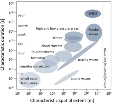
The dynamical processes in the atmosphere (and at the land surface and in the subsurface) act at intrinsic spatial and temporal scales. Turbulent eddies have a spatial extension of sev-eral centimeters to a few hundred meters and a life span between seconds and a few minutes; convective events occur over a wide range of scales from several meters to several kilometers with durations between minutes and hours; large scale oscillation patterns, such as the El Niño and La Niña phases of the El Niño Southern Oscillation ENSO typically persist over several months (cf. Fig. 1.1).

Numerical models are used to simulate the dynamical and physical processes in the atmo-sphere (and at the land or subsurface) in order to make predictions of future weather and climate conditions1 _{and to improve understanding of the interplay of the processes involved.}

Atmospheric models typically rely on a set of prognostic hydro-thermodynamic partial dier-ential equations and a set of diagnostic equations, which together describe the atmospheric state and its change in time. The set of equations is discretized using nite dierences, nite elements etc. or via a spectral approach and solved by numerical integration schemes. Solving the equations is computationally expensive.

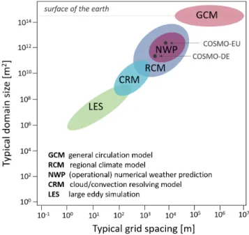
General Circulation Models (GCMs), which cover the whole globe, are therefore restricted to a relatively coarse grid spacing (typically in the order of 100 kilometers) by the available com-putational power. In climate modeling, regional climate models (RCMs) use a smaller grid spacing as these are nested into the GCMs and applied over smaller (regional) domains (e.g., continental Europe with a grid spacing of 7 km). The grid spacing can be decreased further by carrying out multiple nesting steps (e.g., up to 3 km for the Alpine region) (cf. Fig. 1.2). Also in operational numerical weather prediction (NWP) such model chains are common. GCMs provide initial conditions (taken from an analysis run) and boundary conditions to limited area model NWP models with a smaller grid spacing typically for continental do-mains (e.g., COSMO-EU covering a European domain with a 7 km grid spacing). Even more local models with smaller grid spacing (e.g., COSMO-DE covering Germany with a grid spac-ing of 2.8 km) receive initial and boundary conditions from the continental scale models. Atmospheric processes that are not resolved by the model resolution - note that for

numer-1_{Weather refers to the short term atmospheric state. Climate refers to long term (30 years or longer) statistics}

(14)

1. Introduction

Figure 1.1.: Important atmospheric processes and their intrinsic spatial and temporal scales (follow-ing e.g., La(follow-ing and Evans, 2011).

ical reasons the eective resolution of a model corresponds to at least four grid boxes - are accounted for by parameterization schemes. GCMs incorporate cloud schemes, most RCM and NWP applications incorporate convection schemes, and even high-resolution simulations with grid spacings of a few hundred meters still require turbulence schemes. In large eddy simulations (LES) of the atmospheric boundary layer, which is feasible for very small domains only, the large eddies, which are responsible for the major part of the turbulent exchange of mass, energy and momentum, are resolved. However, the smaller eddies, typically in the inertial subrange, are parameterized even in LES simulations.

With the atmosphere being a (deterministic) chaotic system2 _{its numerical modeling is}

in-evitably subject to large uncertainties. Overall uncertainty results from uncertainties of initial and boundary conditions, and uncertainties induced by numerical discretization and parame-terization schemes. Especially the latter are known to constitute a major source of uncertainty. GCMs often have diculties with the representation of clouds and precipitation. In higher resolution models the representation of convection and turbulent exchange of energy, moisture and momentum are still challenging.

Modeled atmospheric data is of use to many communities. The value of modeled atmospheric data to other communities is limited by uncertainty (and potentially systematic errors) and by the available grid spacing. Hydrological models, land surface models, agricultural models etc. require atmospheric data often at high spatial resolutions as many hydrological and land surface modeling applications use a small grid spacing (100 m or less) to account for the heterogeneity of land surface and soil at small scales. Using coarser-scale atmospheric data as forcing for such simulations can induce biases for example in the estimation of the turbulent

2_{Deterministic chaos refers to systems for which any small change in the initial state can (after some time)}

(15)

Figure 1.2.: Domain extent and grid spacing of common types of atmospheric models.

uxes as the uxes are described by nonlinear functions of the state of the land surface and the lowermost atmosphere. With increasing computational power integrated modeling platform coupling subsurface, land surface and atmospheric models are used more and more frequently. For computational reasons and to improve the simulation of the turbulent exchange uxes such platforms often employ mosaic approaches (assigning several land and subsurface grid boxes to one atmospheric model column). An appropriate atmospheric downscaling might further improve the ux estimation as well as the simulation of threshold dependent processes such as snow melt or soil freezing. Moreover, climate change impact modeling (vegetation modules, crop modules, hydrological modules etc.) requires local (up to point scale) atmo-spheric information.

To match the requirements of the users, modeled atmospheric data is often processed using model output statistics, e.g., for bias correction, to reduce systematic errors. The discrep-ancy between required resolution and available resolution from the models (representativeness problem) is addressed by downscaling techniques3_{. In practice many downscaling techniques}

combine the correction of model errors and representativeness problem. For regionalized or local climate projections, a vast number of empirical-statistical downscaling techniques have emerged over the past decades.

The multi-objective Genetic Programming (MOGP) approach presented in this study diers from the majority of downscaling techniques in two ways: (1) Genetic Programming allows the implementation of symbolic regression. That is, model structure and model parameters are evolved simultaneously, such that nonlinear and multivariate predictor-predictand relations can be exibly accounted for. For most present techniques (e.g., most regression approaches,

3_{The nesting of regional climate models into general circulation models is referred to as dynamical}

(16)

1. Introduction

analog techniques) the model structure has to be predened and only the model parameters are optimized. (2) Most existing techniques either aim at matching modeled and reference probability distributions (e.g., quantile mapping or stochastic weather generators) or aim at a pointwise match of the reference data (e.g., most regression techniques including neural networks). The multi-objective approach allows to incorporate multiple tness/cost function when tting the downscaling model. That is, distribution based measures, such as the inte-grated quadratic distance, can be considered together with measures comparing reference and prediction pointwise, such as the root mean square error.

The presented work has been carried out in the framework of the Transregional Collaborative Research Center 32 on Patterns in Soil-Vegetation-Atmosphere-Systems. Initial motivation of the work is the development of an improved atmospheric downscaling scheme to be applied in fully coupled subsurface-land surface-atmosphere simulations with the Terrestrial Systems Modeling Platform (TerrSysMP) developed within TR32. During the work on this thesis the COST action VALUE on Validating and Integrating Downscaling Methods for Climate Change Research has set up a set of downscaling experiments for climate data aiming at a comprehen-sive intercomparison of existing downscaling techniques which has motivated an additional application of MOGP.

The Chapters 2-4 oer background information on the dierent aspects involved in this work. Chapter 2 introduces Genetic Programming and can be skipped by readers familiar to GP. Chapter 3 provides background information on the integrated modeling of the soil-vegetation-atmosphere system focusing on the representation of land-surface heterogeneity, existing mospheric disaggregation approaches and introduces the TerrSysMP. Furthermore, the at-mospheric component model of TerrSysMP, COSMO, which has been used for this study, is described in more detail. Downscaling approaches, mainly designed for downscaling of cli-mate data, are reviewed in Chapter 4. The MOGP downscaling approach is introduced in Chapter 5. The detailed setup and the results of MOGP for downscaling near-surface at-mospheric elds (from 2.8 km to 400 m grid spacing) are described in Chapter 6. For this MOGP application high-resolution modeled data serves as reference. Thus, the downscaling aims to account purely for the representativeness problem ignoring potential model errors. In Chapter 7 we apply MOGP to the rst experiment set up by COST-VALUE, which considers the downscaling of climate data time series from GCM scale to point scale. For this appli-cation observation data serves as reference. Hence, the downscaling accounts for both, the representativeness problem and potential model errors, simultaneously without distinguishing between the two. The major results of this thesis and their implications are summarized and discussed in the conclusion in Chapter 8. Parts of Chapter 5, 6 and Appendix A are published in Simmer et al. (2015) and Zerenner et al. (2016).

(17)

2

Genetic Programming

Genetic Programming addresses the problem of automatic programming, namely, the problem of how to enable a computer to do useful things without instructing it, step by step, how to do it (John R. Koza in Banzhaf et al., 1997).

Genetic Programming (GP) automatically creates program code to solve user dened tasks requiring only a minimum of information by the user. In particular the user is not required to prescribe the size and shape of the solution. GP belongs to the evolutionary computation techniques, which are based on the Darwinian concept of survival of the ttest.

For a given problem a generation of initial solutions is created randomly (or incorporating prior knowledge). Each of these candidate solutions is applied to the problem and evaluated. The solutions from the existing generation are then modied to form a new generation (cf. Fig. 2.1). The better a candidate solution performs, the more likely it contributes to the successive generation. The evolution is stopped and the best solution found returned when a certain number of generations dened by the user is reached (or when a solution is found that performs suciently well).

Evolutionary computation contains not only GP, but also many related techniques such as genetic algorithms (GA) or gene expression programming (GEP). In this work we stick to the classical (tree-based) Genetic Programming. The content of this chapter largely relies on the textbooks by Banzhaf et al. (1997), Mitchell (1998), Poli et al. (2008), Aenzeller et al. (2009) and the pioneering work by Koza (1992). After introducing the fundamental elements

generate population

of programs evaluate their qualityrun programs and

breed better programs

solution

Figure 2.1.: Concept of Evolutionary Computation: Given a problem to solve, a population of potential solutions is frequently tested and updated until the termination criterion is met (Figure adapted from Poli et al., 2008).

(18)

2. Genetic Programming

of a GP system and the associated terminology (Sec. 2.1), we walk through a standard GP algorithm step by step (Sec. 2.2). Finally some real world applications of GP are presented (Sec. 2.3).

2.1. Terminology and Definitions

Parse tree In classical GP the solutions (individuals) are represented by parse trees, which consist of functions and terminals. Each element of a parse tree is also referred to as a node. Figure 2.2 shows an example of a parse tree representing a simple equation. The tree consists of 9 nodes arranged on 4 levels. Parse trees are read bottom to top. That is, the parse tree in Figure 2.2 is evaluated as follows:

(1) 4 is multiplied with c, (2) 2 is divided by 3,

(3) the result of (2) is multiplied with b, (4) the results of (1) and (3) are subtracted.

Hence, the parse tree represents the equation4c−2₃b. This is a simple example of a parse tree containing only arithmetic functions (minus,times,divide), variables (c,b) and constants (2, 3, 4). Dependent on the problem to solve, parse trees can be much larger and much more complex. minus times times divide 2 3 b 4 c

Figure 2.2.: Example of a parse tree representing the simple equation4c−2

3b.

Terminal set The terminal setTprovides the basic input to the parse trees. Thus, terminals

terminate the branches of the tree. The terminal set can contain numerical constants, variables (for instance in regression problems) and any kind of zero-argument functions. In the example parse tree shown in Figure 2.2 the terminals used are the numerical constants 2, 3 and 4, and the variables band c.

Function set The function set F contains all of the functions and statements available to

the GP system. The type of functions can be very diverse. Examples of possible functions and statements are:

Arithmetic functions, i.e., plus, minus, multiply, divide,

(19)

2.1. Terminology and Denitions Boolean functions, i.e., AND, OR, NAND, NOR,

Conditional statements, e.g., IF ... THEN ... ELSE ..., Loop statements, e.g., FOR ... DO ...,

Subroutines.

In the example parse tree shown in Figure 2.2 the function used are subtraction (minus), multiplication (times) and division (divide).

Arity The arity of a function is the number of input arguments. All elements of the terminal set have arity zero. The elements of the function set have an arity of at least one.

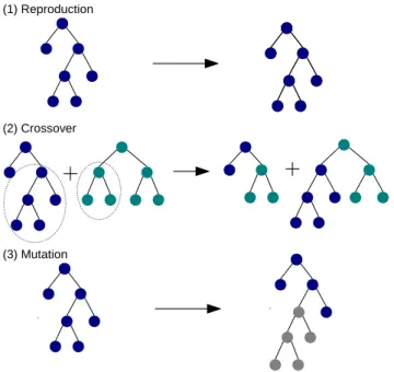
Genetic Operators During the evolutionary process, again and again new populations of candidate solutions are created from the already existing ones by applying genetic operators. The three standard genetic operators commonly used in tree-based GP are:

(1) Reproduction The reproduction operator is the most straightforward. An individual is selected from the current generation, copied and inserted into the new population (cf. Fig. 2.3).

(2) Crossover The crossover operator combines two individuals (parents). At rst two individuals from the current generation are selected to serve as parents. From each par-ent a subtree is chosen randomly. The subtrees are exchanged (cf. Fig. 2.3). Crossover transforms two existing individuals into two new individuals.

(1) Reproduction

(2) Crossover

(3) Mutation

Figure 2.3.: The three common genetic operators used in standard (tree-based) Genetic Program-ming.

(20)

(3) Mutation Mutation operates on one individual only. There are several variants of the mutation operator. In our algorithm we use the standard subtree-mutation. An individual from the current generation is selected. From this individual a randomly chosen subtree is cut o and replaced by a new randomly generated subtree (cf. Fig. 2.3). The mutation operator allows new program sequences to enter the evolutionary process.

Fitness function The tness or tness function is the measure used in GP to quantify how well a candidate solution solves the problem given and is used to evaluate the candidate solutions. During the evolutionary process the tness also determines how likely an individual is selected to serve as parent in the creation of a new generation. The most simple way is to set the selection probability of the individuals proportional to their tness.

2.2. Preparing and Running GP

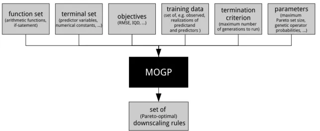
Preparation Figure 2.4 illustrates input and output of a standard GP system. The user provides function and terminal sets. An appropriate selection of functions and terminals is of great importance to successfully employ GP to solve a given problem. Further, a sucient set of training data has to be supplied. The outcome is evaluated by the tness function. Like the denition of functions and terminals, also an appropriate tness function is essential to a successful GP setup. The user can specify some additional run parameters, such as the size of each population, maximum number of levels or nodes for the parse trees or the selection properties of reproduction, crossover and mutation operators. Finally, a termination criterion has to be provided that denes when to stop the GP run. The termination criterion can be reaching a certain tness value or a certain number of generations.

GP

terminal set

function set _functionfitness training data termination_criterion parameters

solution (program code)

Figure 2.4.: Illustration of input and output to Genetic Programming. What happens inside the black box is shown in Fig. 2.5 and explained in the text.

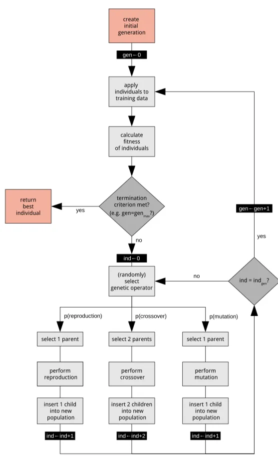
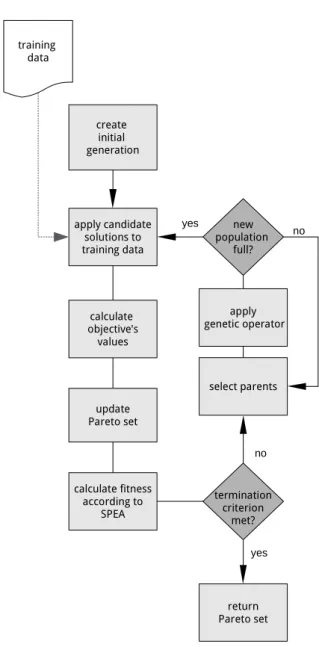
Execution Figure 2.5 shows the typical structure of a GP system. The number of gen-erations run so far is saved as the variable gen. The termination criterion is indicated by genmax, the maximum number of generations to run. The number of individuals in the

cur-rent generation is saved as the variableind. The number of individuals in each generation is indgen.

(21)

2.2. Preparing and Running GP select 1 parent no yes gen←0 apply individuals to training data termination criterion met? (e.g. gen=gen_max?)

calculate fitness of individuals select 2 parents (randomly) select genetic operator select 1 parent perform reproductionperform

reproduction crossoverperform mutationperform

insert 1 child into new population insert 2 children into new population insert 1 child into new population ind←0

ind←ind+1 ind←ind+2 ind←ind+1

ind = ind_gen?

yes create initial generation gen←gen+1 p(mutation) p(crossover) p(reproduction) return best individual no

Figure 2.5.: Flowchart of the main steps of Genetic Programming. A detailed description can be found in the text.

(22)

(1) First an initial population (generation 0) of candidate programs is generated. The variable gen is set to zero, i.e., gen _←0. The initial generation can be created either randomly or include already known approximate solutions of the given problem. (2) The individuals are applied to the training data provided by the user.

(3) The outcome of each individual is evaluated according to the tness function.

(4) If the termination criterion is met (e.g., if the maximum number of generations is reached or if a satisfactory solution is found) the algorithm stops and and the best individual is returned. If the termination criterion is not met, the algorithm continues with the creation of a new, hitherto empty (ind←0), generation:

(a) A genetic operator is randomly selected based on the selection property p.

(b) Depending on the operator selected one or two parents are drawn from the current generation.

(c) The genetic operator is applied to the parent(s).

(d) The ospring is inserted into the new population. That means the number of individuals in the new population is increased by one (ind←ind+1) for mutation or reproduction, or by two (ind←ind+2) for crossover.

(e) Starting from (a) this sequence is repeated until enough individuals for the new generation have been created (i.e., until ind=indgen).

(5) After the new generation is created the algorithm continues at (2).

2.3. Real World Applications

Over the years GP has been applied to a variety of real world problems. Based on thousands of GP applications over the last decades, some criteria have emerged indicating if GP is likely to be a suitable method for a problem (e.g., Poli et al., 2008). GP is likely to perform well

when the relation between the relevant variables is either unknown or at least not fully understood,

when nding the shape and size of the solution is a mayor part of the problem, when sucient amounts of training/test data are available,

when there are good possibilities to test the performance of a candidate solution, but poor chances to directly obtain a sucient solution,

when conventional mathematics do not (or can not) provide an analytic solution, when an approximate solution is acceptable (or the only solution that is ever likely to

be obtained),

(23)

2.3. Real World Applications

Symbolic Regression Many real world applications of GP are symbolic regression prob-lems. Symbolic regression refers to the tting of observed data with the structure of the regression model unknown. Symbolic regression is often used for data where the underlying process is not known or not yet understood well enough to describe it in terms of a mathe-matical formula. Symbolic regression has been one of the earliest applications of GP (Koza, 1992). Common tness functions of symbolic regression problems are the mean error or the root mean square error between the output of the GP solutions and the desired outcomes as contained in the training data set.

Regression problems occur in almost any scientic area (and not only there). Also the detec-tion of downscaling rules considered in the later chapters of this work ranks among the sym-bolic regression problems. Here, mappings are established which predict the high-resolution data from coarser-resolution information using observed or modeled data at high-resolution for training.

Image and Signal Processing In the area of image and signal processing GP has been used, for instance, to visually classify objects (e.g., Smart and Zhang, 2003), for content based image-retrieval (e.g., Torres et al., 2009) or to detect certain image features (e.g., Tackett, 1993).

Compression and Data Mining So called programmatic compression has been already considered in Koza (1992). Programmatic compression treats an image as a function of row and column index of each pixel. Such functions can be derived using GP and serve as a lossy1

compressed version of an image. The technique of programmatic compression has been further studied and applied to both images and sounds in Nordin and Banzhaf (1996). Lossless2_image

compression using GP has been rst considered in Fukunaga and Stechert (1998) who evolve non-linear models predicting the value of a pixel from a subset of neighboring values. Kattan and Poli (2008) proposed a lossless data compression in which GP combines well known compression algorithm such that optimal reduction of the le length is achieved.

Bioinformatics and Medicine A large number of studies considers classication and data mining for large biomedical data sets, such as gene microarray data, by means of GP (e.g., Hong and Cho, 2006; Yu et al., 2007).

Economic Modeling In the economic sector GP has been, for instance, employed for evolv-ing tradevolv-ing rules (e.g., Yu et al., 2005) or to predict stock indices (e.g., Chen et al., 1999).

Geosciences Compared to other areas, such as bioinformatics or economics, GP has been rarely applied to geoscientic tasks. Parasuraman et al. (2007) and Kim and Kim (2008), for

1_{In lossy le compression certain information is permanently eliminated (especially redundant information).}

When the le is uncompressed, only a part of the original information is available. Applied for instance to a graphic lossy compression typically reduces the resolution the graphic.

2_{In lossless le compression no information from the original le is lost. When the le is uncompressed, the}

(24)

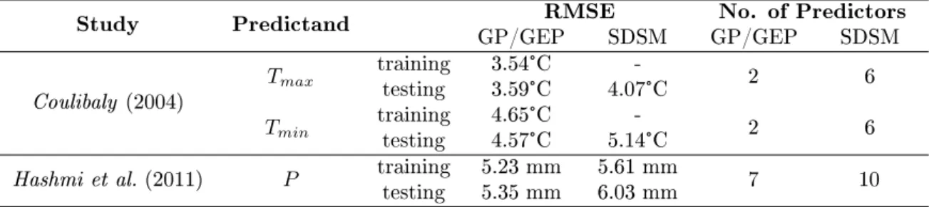
instance, use GP (or genetic algorithms) for evapotranspiration modeling. Wang (1991) em-ploy genetic algorithms for calibrating conceptual run-o models. The few studies emem-ploying GP to the downscaling of general circulation model output (Coulibaly, 2004; Liu et al., 2008; Hashmi et al., 2011) are reviewed in detail in Section 4.4.

(25)

3

Integrated Modeling of the Soil-Vegetation-Atmosphere

System

The Transregional Collaborative Research Center 32 studies Patterns in Soil-Vegetation-Atmosphere Systems using monitoring, modeling and data assimilation (Vereecken et al., 2010; Simmer et al., 2015). Processes in soil, vegetation and atmosphere act over a large range of spatial and temporal scales. The land surface is strongly heterogeneous with respect to topography and texture with especially the latter being strongly aected by human usage. Typically atmospheric models are computationally signicantly more expensive than land surface and subsurface models and therefore applied with comparatively coarse grid spacings. Eects of subscale land surface heterogeneity on the turbulent exchange between land surface and atmosphere can be partly accounted for by parameterization schemes. An overview of the treatment of land surface heterogeneity in atmospheric modeling is given in Section 3.1. Not only the land surface is strongly heterogeneous but also the lower atmospheric boundary layer, which is signicantly inuenced by land surface heterogeneity. Atmospheric disaggre-gation or subgrid-scale parameterizations aim to account for the spatial variability in the low-ermost atmosphere with the ultimate goal of scale-consistent coupling between atmospheric models and surface (and subsurface) schemes or models. In Section 3.2 existing approaches are reviewed with a special focus on the 3-step downscaling scheme by Schomburg et al. (2010), which has been developed in the rst phase of TR32. The 3-step scheme has been designed for downscaling mesoscale near-surface atmospheric elds from 2.8 km to 400 m grid spacing. In the central step of the scheme, which aims to reconstruct the ne-scale structures of the elds, a linear regression utilizing high-resolution land surface information is applied. The 3-step scheme performs well for a subset of the atmospheric state variables required by land surface and subsurface models and/or under certain weather conditions. By applying MOGP to the downscaling of atmospheric near-surface elds at the mesoscale, we aim to account also for complex and nonlinear processes in the lower atmospheric boundary layer, which cannot be captured by a simple linear regression (cf. Chap. 6).

During the second phase of the TR32 the integrated Terrestrial Systems Modeling Platform (TerrSysMP) has been set up by Shrestha et al. (2014). TerrSysMP oers a highly modular platform coupling the atmospheric model COSMO, the land surface model CLM and the sub-surface model ParFlow via an external coupling interface. In Section 3.3 TerrSysMP and its

(26)

3. Integrated Modeling of the Soil-Vegetation-Atmosphere System

components are briey introduced. In the current setup TerrSysMP optionally includes the 3-step downscaling algorithm by Schomburg et al. (2010).

To improve the downscaling algorithm a new and larger reference data set has been created by carrying out high-resolution simulations (400 m grid spacing) with the most recent version of the COSMO model. The COSMO model is thus reviewed in more detail in Section 3.4 focusing on the COSMO-DE conguration, which has been adapted for the high-resolution simulations (cf. Sec. 6.1.1).

3.1. Land Surface Heterogeneity in Earth System Modeling

The land surface is an important constituent of the earth system as it represents the inter-face between atmosphere, biosphere and subsurinter-face hydrology. The land surinter-face exchanges momentum, energy, and water and other constituents, such as CO2, with the atmosphere and thus impacts weather and climate. In atmospheric modeling so-called soil-vegetation-atmosphere transfer schemes (SVATs) are used to capture these interactions. Typical SVATs are composed of sub-models (soil modules, vegetation modules, snow modules, land surface hydrology modules) interacting with the atmosphere and with each other. SVATs calculate the surface-atmosphere exchange uxes of momentum, energy (radiation, sensible heat, la-tent heat), moisture and other constituents, such as CO2, as lower boundary condition to the atmospheric models.

The accurate representation of the turbulent exchange uxes in models is challenging as the uxes result from an interacting chain of parameterized processes above and below the land surface (e.g., Schomburg, 2011). The turbulent exchange uxes are typically parameterized following the Monin-Obhukov similarity theory (e.g., Stull, 2012). Monin-Obhukov theory describes turbulent motion within the lower atmosphere above homogeneous terrain. In real-ity the land surface is not homogeneous, but heterogeneous with respect to many parameters and over a wide range of spatial scales. Land surface heterogeneity is created by:

vegetation cover and surface type (vegetation, bare soil, urban area, etc.), terrain morphology (elevation, slope, orientation),

soil characteristics,

variability of climatic forcings (e.g., spatial precipitation patterns)

(Giorgi and Avissar, 1997). The heterogeneity of the land surface aects the land-atmosphere exchange of energy, momentum, moisture and other constituents and thus impacts energy and moisture budgets. The turbulent exchange over forested areas is typically much stronger than over bare soil areas. This is, rstly, due to the much larger roughness of forests leading to a more pronounced coupling between land surface temperature and near-surface air temper-ature. Secondly, the roots of the trees can access deep soil moisture reservoirs leading to moister conditions in the lower atmosphere compared to bare soil areas caused by transpi-ration (Schomburg, 2011). This is just one example of how the turbulent exchange uxes are aected by land surface characteristics. Idealized simulations with a mesocale model by

(27)

3.1. Land Surface Heterogeneity in Earth System Modeling Avissar and Pielke (1989) have shown, for instance, strong dierences for (maximum) latent and sensible heat uxes over dierent surfaces (460 W/m2 _{dierence between sensible heat} uxes over water bodies and urban areas; 610 W/m2 _{dierence between built up areas and} cropland). Measurement campaigns have conrmed large dierences in the turbulent uxes for dierent land surfaces (e.g., LITFASS Lindenberg Inhomogeneous Terrain - Fluxes between Atmosphere and Surface, Beyrich and Mengelkamp, 2006 ; EVA-GRIPS Evaporation at Grid and Pixel Scale, Mengelkamp et al., 2006).

Atmospheric models are computationally expensive and therefore limited in grid spacing. Even with increasing computational power (and smaller grid spacing) the land surface re-mains heterogeneous at the subgrid-scale. Many eects induced by subgrid-scale land surface heterogeneity can be parameterized (e.g. Avissar and Pielke, 1989; Avissar, 1992; Koster and Suarez, 1992; Seth et al., 1994; Leung and Ghan, 1995; Schlünzen and Katzfey, 2003; Heine-mann and Kerschgens, 2005; Ament and Simmer, 2006).

The eects of land surface heterogeneity are often split into aggregation and dynamical eects (e.g., Giorgi and Avissar, 1997). Aggregation eects occur when two land surface processes F and Gare nonlinearly dependent on the heterogeneous surface variablesx,y such that the grid box averaged eect of x on F cannot be represented by averaging x over the grid box and than applyingF, i.e.,

F(x)6=F(¯x);G(x)6=G(¯x)

and such that combined eects of heterogeneity ofx on F and y on G cannot be calculated from the averaged eects ofF(x) andG(y), i.e.,

F(x)G(y)₆=F(x) G(y)₆=F(¯x)G(¯y).

Aggregation eects have been shown to aect latent and sensible heat uxes as well as the simulation of snow, soil moisture dynamics and runo as all these processes exhibit a nonlin-ear dependency on land surface characteristics and/or state variables at the surface and/or the lower atmosphere. The use of averaged parameters and state variables can introduce sig-nicant biases when simulating such processes. Aggregation eect models aim to reduce these biases by calculating the contribution of subgrid-scale heterogeneity to the grid box average of land-atmosphere exchange uxes, water budgets and so on.

Dynamical eects are associated with micro- and mesoscale circulations induced by land sur-face heterogeneity. These can inuence the boundary layer structure and the vertical transport of momentum, energy and water. Models of dynamical eects attempt to simulate the rele-vant impacts of the land surface heterogeneity induced micro- and/or mesoscale circulations. In coarser-scale models with a grid spacing in the order of 10-100 km both dynamical and aggregation eects are not suciently resolved. In smaller-scale models, such as the COSMO-DE (2.8 km grid spacing), dynamical eects are explicitly modeled to some degree. However, the aggregation eects remain relevant also for grid spacings of few kilometers, as surface heterogeneity is present down to very small scales.

Aggregation methods seek to parameterize aggregations eects and can be split into two classes, the discrete methods and the PDF methods. The discrete methods (tile and mosaic

(28)

approaches) divide each model grid box into a number of homogeneous subregions denoted as tiles or patches. The surface calculations are carried out separately for each tile and after-wards aggregated to the full model grid box by computing an area weighted average over all tiles/patches. In the PDF methods the parameters and variables which are heterogeneous on the subgrid scale are described by either analytically or empirically derived PDFs. Aggrega-tion is then carried out in the phase space spanned by the parameter's PDFs.

Tile approaches (e.g., Avissar and Pielke, 1989; Koster and Suarez, 1992)1 _{divide the model}

grid box into a number of homogeneous tiles that exchange uxes with the atmosphere directly and independent of each other. The subgrid-scale tiles can be dened based on vegetation types (Koster and Suarez, 1992), topographic elevation (Leung and Ghan, 1995) or via a combination of dierent land surface characteristics such as vegetation, soil, slope orientation and so on as in Avissar and Pielke (1989). Tile schemes do not keep track of exact location of the tiles.

In the explicit subgrid approach by Seth et al. (1994) each model box is divided into N2 subgrid elements (cf. Fig. 3.3), i.e., a higher-resolution land surface scheme is nested into the coarser-resolution atmospheric model. In the following the explicit subgrid scheme is also referred to as mosaic scheme. In Seth et al. (1994) each subgrid cell is governed by a single vegetation type (either the most frequent one or a type whose characteristics match the char-acteristics averaged over all surface types) and bare soil. The main dierence between tile and mosaic approach is that in the mosaic approach each subgrid cell is assigned a specic location. Thus, climatic forcing can be explicitly distributed over the subgrid cells. The basic assumption motivating the discrete mosaic is that subgrid-scale climatic forcing experienced by the land surface is important for the calculation of net exchange of heat, moisture, momen-tum. Still, the subgrid-scale heterogeneity of the surface does not penetrate vertically above the surface layer. The atmosphere only sees the eective uxes and dynamical eects are not accounted for.

3.2. Atmospheric Disaggregation

In most studies applying tile or mosaic approaches (e.g., Avissar and Pielke, 1989; Koster and Suarez, 1992) grid box averaged atmospheric forcing is applied to each subgrid tile or grid cell, i.e., no atmospheric disaggregation is carried out. However, the lower atmospheric boundary layer is known to be highly heterogeneous especially above heterogeneous land surfaces even down to small scales (below 1 km).

Pitman et al. (1993) have investigated the eects of the assumption of constant precipitation over the subgrid-scale tiles in GCM simulations. The authors have compared simulations with constant precipitation over each grid box with simulations where precipitation has been disaggregated such that only a fraction of each grid box is governed by precipitation. The intensity has been disaggregated as the grid box average precipitation divided by the pre-cipitation fraction. It has shown that prepre-cipitation disaggregation can have a huge impact

1_{Tile approaches are sometimes also referred to as mosaic approaches. When we talk of mosaic approaches}

(29)

3.2. Atmospheric Disaggregation on runo simulation. The simulated water budget changed from evaporation dominated to runo dominated. Other studies showed less sensitivity to fractional precipitation disaggrega-tion (Giorgi, 1997a,b), which might be due to dierent runo parameterizadisaggrega-tions. Hydrological models often operate at even higher resolutions than land surface schemes. Several studies, for instance by Singh (1997) and Segond et al. (2007), have conrmed the importance of a realistic distribution of precipitation for evaporation and runo simulation.

Not only the subgrid-scale variability of precipitation aects the simulation of land surface and subsurface processes, but also the subgrid-scale of near surface temperature, humidity, wind speed and incoming radiation aects land and subsurface. Shao et al. (2001) have examined the eects of both land surface heterogeneity and near surface atmospheric heterogeneity on the simulation of the surface energy and momentum uxes with a mesoscale model. A series of numerical experiments has been carried out over a domain of40_×40 km centered around

Cologne. In the simulations dierent grid spacings (1 km, 2 km and 4 km) for atmosphere and land surface have been used. It has shown that not only an increased grid resolution of the land surface for a given atmospheric grid resolution improves the simulation of the uxes, but also an increased atmospheric grid resolution for a given land surface grid resolution leads to an improved ux estimation. While the former is widely agreed on, the latter contradicts the often prevailing view that atmospheric subgrid variability especially on smaller scales (e.g., in meso-γ scale weather prediction) only plays a minor role compared to the land surface het-erogeneity itself. Subgrid atmospheric motions (and thus variability) might be an important factor to be included in subgrid closure schemes of atmospheric models.

3.2.1. Early Approaches

The discrete (mosaic) scheme (Seth et al., 1994) allows the usage of explicitly distributed atmospheric forcings. Seth et al. (1994) have applied a simple disaggregation for temperature, humidity and convective clouds and precipitation. Temperature and humidity have been either downscaled proportional to soil temperature or soil moisture anomalies or based on topographic height anomalies. The simulations have been carried out with very coarse grid spacing of approximately 30° (≈300 km) for the atmosphere and 5° (_≈50 km) for the land

surface. For simulations over 20 years the atmospheric disaggregation has changed the heat uxes up to 15% and runo up to 33%.

Giorgi et al. (2003) have adapted the approach of Seth et al. (1994) for simulations with a regional climate model over the Alpine region with a 60 km grid spacing for the atmosphere and a 10 to 15 km grid spacing for the land surface. Near-surface atmospheric temperature and specic humidity have been downscaled based on topographic height. Convective precipitation has been distributed over one randomly chosen third of the subgrid-scale pixels. The analysis of an 11 months simulation has shown an improved near-surface temperature over the complex Alpine terrain and a more realistic representation of snow patterns, which may lead to a better simulation of the seasonal evolution of the surface hydrology.

Molod et al. (2003) have presented a technique called extended mosaic. In the extended mosaic not only the land surface processes are simulated in the subgrid-scale tiles, but also turbulent motion in the boundary layer. A comparison of GCM simulations with the standard land

(30)

surface mosaic and the extended mosaic have shown large dierences for various regions all over the globe (Molod et al., 2004).

3.2.2. The Schomburg 3-Step Scheme

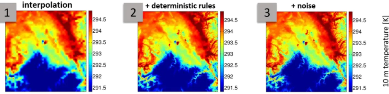
The downscaling scheme of Schomburg et al. (2010) has been developed for downscaling near-surface atmospheric elds from 2.8 km to 400 m scale and consists of three steps. The three steps can be applied consecutively or individually for stand-alone oine simulations as well as in a fully coupled model system, such as TerrSysMP (Shrestha et al., 2014). In the rst step, a biquadratic spline interpolation is used to interpolate the coarse-scale atmospheric data to a higher resolution while conserving mean and horizontal gradients of the coarse eld. In the second step, deterministic downscaling rules are applied to the interpolated eld. The rules are based on relations between atmospheric variables and the high resolution surface information. In the last step, autoregressive noise is added to the eld to restore the high resolution variance of the elds (cf. Fig. 3.1).

Step 1: Spline interpolation

The biquadratic spline interpolation smooths the coarse eld and can be written as

yij =y(i, j) =a1+a2i+a3j+a4i2+a5j2, (3.1) withy denoting an atmospheric variable, for instance temperature,(i, j)the grid point on the

ne-scale, anda1, ...., a5denoting the regression coecients. To estimate the regression coe-cients ve constraints are introduced: The derivatives of Equation 3.1 at the four edges of the coarse pixel are required to equal the gradient between the coarse pixel and the corresponding neighboring pixel. Further, the coarse pixel mean is conserved.

Step 2: Deterministic downscaling rules

The deterministic downscaling rules are applied to estimate the high-resolution anomalies on top of the interpolation. High-resolution surface information serves as predictors in a linear regression. Some of the near-surface atmospheric variables can be downscaled exploiting known physical relationships:

Figure 3.1.: The three steps of the downscaling scheme by Schomburg et al. (2010) applied to a 10 m temperature eld on May 12th 2008, a clear sky day, at 10 UTC (Figures by A. Schomburg).

(31)

3.2. Atmospheric Disaggregation Surface pressure anomaly ∆p is estimated using relief height ∆z as predictor in the

hydrostatic equation

∆p=₋ρg∆z (3.2)

with the assumption of a constant air density ofρ= 1.19 kg/m3.

For cloud free skies the diuse part of upwelling shortwave radiationSdif ↑ is

down-scaled using surface albedo for direct αdir and diuse αdif radiation by

Sdif ↑=αdirSdir↓+αdifSdif ↓ (3.3)

with Sdir↓and Sdif ↓denoting direct and diuse downwelling radiation.

For the remaining ve variables (temperature, wind speed, specic humidity, longwave ra-diation, precipitation) there are no known direct relationships to the surface characteristics. Therefore, the training data set has been evaluated for possible correlations, which usually depend on the prevailing weather conditions. An automatic rule detection system has been set up to nd the best predictors, indicators and thresholds. The system calculates the corre-lations between the 5 predictands and 16 possible predictors given by the surface parameters and elds derived therefrom for dierent subsets of the training data. The selection of the data subsets is based on 24 dierent indicators, e.g., vertical temperature gradients or wind speed below certain thresholds. The system selects only rules achieving correlations above 0.7 and applicable to at least 10% of the data:

For the near surface temperature several rules have been found. The best rule found uses orographic height information for downscaling when the temperature gradient of the lowest 105 m is smaller than 0.0057 Km−1_.

The longwave net radiation can be disaggregated using ground temperature as pre-dictand when the cloud cover is below 43% or when the longwave net radiation is less than -82.5 Wm−2_{. These two indicators are almost equivalent.}

For other weather situations and the remaining variables (specic humidity, wind speed and precipitation) no applicable rules could be found.

Step 3: Noise generation

As many processes at the surface are nonlinear, also the reproduction of variance can be im-portant to reduce biases. Except for the near-surface pressure, steps 1 and 2 do not reproduce all ne-scale variability. Therefore, in step 3 autoregressive Gaussian noise is added to the elds resulting from step 1 and 2. For this a stepwise multiple linear regression has been applied to predict the ne-scale standard deviation from the coarse-scale standard deviation (of the surrounding 3_×3 coarse pixels) of the respective variable and other atmospheric

parameters. The autoregression coecients are obtained from several high-resolution model runs. In the third step spatial correlations are ignored.

(32)

the mean of the downscaled values for each coarse grid cell. This is important to assure that the conservation of energy and mass is not violated by the downscaling. In case the down-scaling predicts unphysical values (e.g., negative wind speeds or negative values for shortwave radiation) the respective values are set to zero or to the coarse pixel mean (for wind speed). In such cases the conservation of the mean is ensured by multiplying the subgrid values by the fraction of the coarse mean before and after correcting the unphysical values.

Precipitation is treated dierently from all other variables since the assumption of Gaussian noise does not model the distribution of the precipitation anomalies well. For precipitation the Gaussian noise term is transformed via an exponential function to match the distribu-tions estimated from two high-resolution model runs that have generated precipitation. The transformed noise terms are multiplied by the coarse pixel mean precipitation.

3.2.3. TopoSCALE

Fiddes and Gruber (2014) have presented a physically based and computationally ecient downscaling scheme called TopoSCALE for gridded climate data in complex terrain. TopoSCALE is foremost aimed at creating high-resolution forcing data for land surface models (≤100m)

from general circulation model output (50-100 km) by using ne-scale topography information from a high-resolution digital elevation model.

Temperature, wind speed and specic humidity are interpolated according to the subgrid-scale topographic height and the vertical gradients of the respective variables, the latter being obtained from the coarse-scale atmospheric model output. For wind speed an additional topographic correction according to Liston and Sturm (1998) is optionally applied.

Shortwave radiation is downscaled using multiple steps. First, shortwave radiation is partitioned into direct and diuse components. Direct shortwave radiation can then be downscaled according to the dierence of the optical path length determined from the topographic heights at grid- and subgrid-scale. Topographic corrections are applied to both diuse and direct radiation at subgrid-scale to account for shadowing eects occurring especially within complex terrain.

Longwave radiation is downscaled in multiple steps. First clear sky emissivity is deter-mined at the grid and subgrid-scale using grid-scale and downscaled (i.e., subgrid-scale) temperature and specic humidity. Next all-sky emissivity at grid scale is determined from the grid-scale longwave radiation and temperature utilizing the Stefan-Boltzmann equation. The dierence between grid-scale clear sky and all sky emissivity provides the correction factor for the subgrid-scale longwave radiation obtained from subgrid-scale temperature according to the Stefan-Boltzmann equation. This approach assumes that cloud emissivity at grid and subgrid elevations are the same, but accounts for the reduc-tion of clear-sky emissivity with height. After the elevareduc-tion correcreduc-tion, terrain eects are accounted for by multiplication with the sky-view factor, i.e., the fraction of the sky visible from subgrid-scale pixel.

(33)

3.3. The Terrestrial Systems Modeling Platform TerrSysMP Precipitation is downscaled assuming a simple nonlinear lapse and optionally utilizing

precipitation climatologies.

TopoSCALE has been tested and compared with unprocessed coarse GCM data and a set of simple disaggregation methods (e.g., assuming a xed lapse rate for temperature). A com-parison for up to 210 local stations in the Swiss Alps has shown signicant improvements for TopoSCALE for air temperature, relative humidity and incoming longwave radiation com-pared to the reference methods.

3.2.4. VERTEX

Recent studies by de Vrese and Hagemann (2016) and de Vrese et al. (2016) suggest a con-ceptually dierent approach called VERtical Tile EXtension (VERTEX), which can be seen as an advancement of Molod et al. (2003). VERTEX expands the concept of the tile approach into the vertical. Horizontal homogeneity is thus explicitly considered not only at the land surface, but also within the lower atmospheric model layers, where turbulent mixing is cal-culated for the single tiles dened by the dierent land surfaces. In addition to Molod et al. (2003) also horizontal turbulent exchange between the subgrid-scale tiles is explicitly included in the scheme.

In de Vrese et al. (2016) single-column simulations at the GCM scale incorporating the VER-TEX scheme and employing a simple ux-aggregation scheme have been carried out. It has shown that the vertical turbulent transport can largely dier between the subgrid tiles. Further, the comparison of the simulations with and without VERTEX has shown that the horizontal disaggregation of the turbulent mixing process considerably impacts the mean state of the grid box. In the simulations the impact of the explicit subgrid-scale representation of the lower ABL has been, roughly approximated, half as large as for the explicit representation of land surface heterogeneity.

The VERTEX technique is still in an early stage of development, but rst tests suggest that it might oer a promising approach to improve the representation of aggregation eects in coupled land surface-atmospheric simulations. In the rst application (without any compu-tational optimization) a model set up using 14 tiles for both, land surface and atmosphere, models with the VERTEX scheme take almost 40% longer than simulations with a standard ux-aggregation scheme. Thus, computational optimization will be a crucial to make the VERTEX scheme applicable for long term GCM simulations. Studies with smaller grid spac-ings (e.g., for RCMs or mesoscale NWP models) have, to our current knowledge, not yet been carried out.

3.3. The Terrestrial Systems Modeling Platform TerrSysMP

The Terrestrial Systems Modeling Platform (TerrSysMP) by Shrestha et al. (2014), which has been developed within the Transregional Collaborative Research Center 32, oers a highly modular framework for simulations of the soil-vegetation-atmosphere system. TerrSysMP consists of the atmospheric model COSMO, land surface model CLM and the groundwater

(34)

Figure 3.2.: Schematic diagram of TerrSysMP from Shrestha et al. (2014). Atmospheric model COSMO, land surface model CLM and subsurface model ParFlow are coupled via the external coupler OASIS3, which manages the data exchange between the component models ©American Meteorolog-ical Society (AMS).

model ParFlow. The three component models are coupled using the OASIS coupler, which allows for a separation of model grid spacing, time stepping and coupling frequency between the component models (cf. Fig. 3.2).

The lower boundary of atmospheric models is commonly represented by soil-vegetation-atmosphere transfer (SVAT) schemes. From an atmospheric modelers perspective state-of-the-art land surface and groundwater models can oer an improved parameterization of the lower atmospheric boundary and thereby improve the representation of the exchange uxes of energy, moisture and momentum. This is important as these uxes largely aect the evolu-tion of the atmospheric boundary layer. A better understanding and representaevolu-tion of surface uxes might ultimately lead to better atmospheric and hydrological predictions (e.g., Avissar and Pielke, 1989; Betts et al., 1996; Walko et al., 2000; Ament and Simmer, 2006). Recent studies further suggest that the surface uxes can be strongly coupled to groundwater table dynamics (e.g., Maxwell et al., 2007; Miguez-Macho et al., 2007; Anyah et al., 2008; Maxwell and Kollet, 2008; Kollet and Maxwell, 2008; Rihani et al., 2010).

Increasing computational power allows for the use of integrated modeling approaches, such as TerrSysMP, simulating interaction and feedback processes between soil, vegetation and atmosphere. Idealized simulations with TerrSysMP (Shrestha et al., 2014) support previous studies showing a strong linkage between groundwater dynamics, biogeophysical processes and the atmospheric boundary layer. Simulations over the Rur catchment exhibit patterns in root zone soil moisture, which impact turbulent exchange uxes and thus boundary layer evolution. Rahman et al. (2015) have found evidence that, especially under strong convective conditions, groundwater table dynamics can aect atmospheric boundary layer height, con-vective available potential energy, and potentially precipitation. Thus, it appears that not only a sucient representation of land surface processes is crucial to atmospheric modeling, but also the representation of subsurface processes.

(35)

3.3. The Terrestrial Systems Modeling Platform TerrSysMP As the land surface (topography, land cover) and the soil (soil type) are highly heterogeneous at small scales and strongly aect the spatial variability of soil moisture and groundwater table depth, land surface and subsurface/hydrological models are typically applied with a relatively small grid spacing. Grid spacing of typical atmospheric mesoscale models is too large to suciently represent small-scale variability of land surface and soil. Thus, a scale gap between atmosphere and land surface occurs. In modular platforms, such as TerrSysMP, it is common to apply land surface and subsurface models with a higher spatial resolution than the atmospheric model (following the mosaic approach; cf. Fig. 3.3). Not only the use of averaged state parameters at the land surface, but also for the lowermost atmosphere can introduce biases in ux estimation. Downscaling/disaggregation schemes seek to overcome this issue aiming at a more realistic representation of surface uxes and their spatial variability. In the following the component models are briey introduced together with the OASIS cou-pling interface which, for TerrSysMP, optionally incorporates the 3-step downscaling scheme by Schomburg et al. (2010) (cf. Sec. 3.2.2). The COSMO model, which has been applied for this thesis (cf. Chap. 6), is introduced in more detail in the Section 3.4.

COSMO

The COSMO model is a non-hydrostatic limited area model for atmospheric predictions. The basic version of the model has been developed at the German Weather Service ("Deutscher Wetterdienst", DWD). The Consortium of Small-Scale Modeling (short COSMO), which is comprised of several mainly European weather services, coordinates improvements, mainte-nance and applications. The TerrSysMP setup of Shrestha et al. (2014) contains the con-vection permitting model conguration COSMO-DE (Baldauf et al., 2011), which has in its operational setup a grid spacing of 2.8 km.

CLM

The Community Land Model (CLM; Oleson et al., 2004, 2008) is the land surface scheme of TerrSysMP. In the coupled setup, CLM serves as an interface between atmospheric and sub-surface model and calculates the uxes of energy, momentum, moisture and carbon between soil, vegetation and atmosphere. The CLM is a complex land surface model comprised of biogeophysical, biogeochemical, (dynamic) vegetation and simple hydrological components. Biogeophysical processes modeled by CLM include absorption, reection and transmittance of solar radiation; absorption and emission of longwave radiation; momentum, sensible and latent heat transfer from canopy and soil surface; plant physiology and photosynthesis; and canopy, snow and soil hydrology.

The CLM allows for the representation of subgrid-scale surface heterogeneity by a tiling ap-proach with thee subgrid levels: Each CLM grid cell can be comprised of up to ve dierent land cover types (glacier, lake, wetland, urban, vegetation). Each of those land units can have multiple soil columns with distinct soil types. Each soil column can have up to 4 (out of 16 possible) plant functional types (PFTs) with each PFT having its own distinct set of plant physiological parameters.

(36)

Figure 3.3.: Illustration of the scale gap occurring between the atmospheric component model (COSMO), and the land surface (CLM) and subsurface (ParFlow) component models of TerrSysMP. The grid spacings of the single component models can be exibly chosen by the user of TerrSysMP. Using a smaller grid spacing for land and subsurface than for the atmosphere is often reasonable as discussed in the text.

ParFlow

ParFlow is a variably saturated 3D Richardson equation based groundwater ow model with two dimensional overland ow (Kollet and Maxwell, 2006). Recently a terrain following grid transformation with a variable vertical discretization has been implemented (Maxwell, 2013), which leads to signicant reductions in computational cost, especially for regions with distinct topography, and thus allows the use of ner grid resolutions near the surface and within the root zone leading to an improved representation of land surface uxes.

OASIS

The OASIS3 coupler (Valcke, 2013) serves as the coupling interface of TerrSysMP. OASIS allows a highly modular usage of the modeling platform. The TerrSysMP user can not only run the fully coupled system (i.e., COSMO-CLM-ParFlow), but also stand-alone versions of the component models, COSMO only coupled with CLM or CLM coupled with ParFlow with oine atmospheric forcing.

Model denition (model grid, input/output variables, ...) initialization and termination as well as the data exchange between the component models are all organized via the OASIS interface. Coupling frequency, names and spatial grid of the coupling elds as well as potential transformations of the coupling elds are specied in the OASIS conguration le. Time-integration-averaging and spatial interpolation operators are available to transform the 2D coupling elds before transferring them between the component models. Time integration and averaging is used when the coupling time step is larger than a component model time step. In Shrestha et al. (2014) precipitation send from COSMO to CLM is integrated in time and the remaining atmospheric variables are temporally averaged. Spatial interpolation is required

(37)

3.4. The COSMO Model when the coupling variables are dened on dierent grids. COSMO for instance uses a rotated geographical coordinate system, while CLM variables are dened on a regular geographical grid. Thus, the coupling elds exchanged between COSMO and CLM need to be interpolated to the respective grids.

COSMO-CLM At the interface between the atmospheric model COSMO and the land surface model CLM atmospheric forcing terms and surface uxes are exchanged. The state variables of the lowest COSMO layer at the current time step serve as forcing for CLM. The COSMO model sends temperature T, horizontal wind speed wh, specic humidity q, (convective and

grid scale) precipitation P, pressure p, incoming direct and diuse shortwave SW Rdir and

SW Rdif and incoming longwave radiation LW Rdif. CLM then calculates the surface uxes

of latent and sensible heatLHandSH, momentum uxesτ, albedoαand outgoing radiation LW and sends them back to COSMO (cf. Fig. 3.2). The estimated uxes are used to update the (dimensionless) transfer coecients of heat and momentum at the surface in COSMO. In TerrSysMP the existing tile approach for CLM is not used. Instead a mosaic approach is employed where each atmospheric grid cell contains multiple land surface grid cells. In the mosaic each CLM grid cell is homogeneous. That is, each grid cell is assigned one PFT, one soil column and one land unit. The mosaic approach allows to combine the simulation of subsurface hydrodynamics with overland ow as done by ParFlow. Furthermore, the mosaic allows the use of distributed atmospheric forcings. In the current version of TerrSysMP atmospheric downscaling according to Schomburg et al. (2010) is available as an optional component of the OASIS interface.

CLM-ParFlow In the coupled mode ParFlow, with its 3D variably saturated groundwater representation and its free surface overland ow boundary condition, computes surface runo and subsurface hydrodynamics, which allows for a exibl