Music Generation using Convolutional
Restricted Boltzmann Machines and Constraints
Stefan Lattner1,2, Maarten Grachten1 and Gerhard Widmer1,2
1Department of Computational Perception, Johannes Kepler University, Linz, Austria 2
Austrian Research Institute for Artificial Intelligence, Vienna, Austria
Abstract We introduce a method for imposing higher-level structure on generated, polyphonic music. A Convolutional Restricted Boltzmann Machine (C-RBM) as a generative model is combined with gradient des-cent constraint optimisation to provide further control over the genera-tion process. Among other things, this allows for the use of a “template” piece, from which some structural properties can be extracted, and trans-ferred as constraints to the newly generated material. The sampling pro-cess is guided with Simulated Annealing to avoid local optima, and to find solutions that both satisfy the constraints, and are relatively stable with respect to the C-RBM. Results show that with this approach it is possible to control the higher-level self-similarity structure, the meter, and the tonal properties of the resulting musical piece, while preserving its local musical coherence.
Keywords: Constrained Sampling, Convolutional Restricted Boltzmann Ma-chine, Music Generation, Optimisation
1
Introduction
For centuries, mathematical formalisms have been used to generate musical ma-terial (Kirchmeyer,1968). Since computers can automate such processes, auto-matic music generation has become a small, but steadily emerging field in Arti-ficial Intelligence and Machine Learning. Nevertheless, automatic music genera-tion as a problem is far from solved: musical outputs created by artificial systems are regarded as a curiosity by human listeners at best, but all too often they are taken as a direct offence to our sense of musical aesthetics. This sensitivity to violations of even the most subtle musical norms illustrates how complex the problem of (especially polyphonic) music generation is. In addition, there are only a few objective evaluation criteria to rigorously test and compare music generation systems, all of which involve human judgement (Jordanous, 2012; Pearce & Wiggins,2001).
or representations such as monophonic folk melodies (Sturm, Santos, Ben-Tal & Korshunova,2016), symbolic chord sequences, or drum tracks (Choi, Fazekas & Sandler, 2016) and even in polyphonic music with clearly defined melodic voices, such as Bach chorales (Boulanger-Lewandowski, Bengio & Vincent,2012; Hadjeres, Pachet & Nielsen, 2017; Liang, Gotham, Johnson & Shotton, 2017; Huang, Cooijmans, Roberts, Courville & Eck, 2017), sequence modelling ap-proaches yield impressive results that are sometimes hard to distinguish from human-composed material.
However, in more complex musical material, such as piano music from the classical (e.g. Mozart) or romantic period (e.g. Chopin, Liszt), not to mention orchestral works, important musical characteristics may defy straight-forward time series modelling approaches. Tonality for example, is the characteristic that music is perceived to be in a particular (possibly time-variant)musical key, implying that some pitches are regarded as more stable than others. Although the perception of musical key is a complex topic in itself, there is evidence that an important determining factor is the frequency of occurrence of pitches in the piece (Smith & Schmuckler,2004).
In addition to tonality, meter is an important aspect of music. Perception of meter is the sensation that musical time can be divided into equal intervals at different levels, and that positions that coincide with the start of higher-level intervals have more importance than those coinciding with lower higher-levels. Analogous to the perception of musical key, the perception of meter is in part related to the distribution of musical events over time (Palmer & Krumhansl,
1990).
Lastly, music often transmits a sense of coherence over the course of the piece, in that it has a structural organisation in which motifs (small musical patterns), but also larger units such as phrases, melodies or complete sections of the music are repeated throughout the piece, either literally or in an altered form. This characteristic is reflected in the self-similarity matrix of the music, where entry (i, j) expresses the similarity between the music at positionsi and
j. This coherence by way of repeating and developing musical material over the course of the piece is arguably one of the aspects of music that make listening and re-listening a valuable experience to human listeners.
time induces a stable musical key over an expanded period of time. It is even more challenging to generate music that exhibits the hierarchical organisational structure common in human-composed music. For instance, the rather common pattern of a melodic line from the opening of a piece being repeated as the conclusion of that piece is very hard to capture, even if state-of-the-art sequence models like LSTMs are capable of learning long-term dependencies in the data. Models that fail to capture these higher-level musical characteristics may still produce music that on a short time scale sounds very convincing, but on longer stretches of time tends to sound like it wanders aimlessly, and misses a sense of musical direction.
In this work, we do not address the problem of learning the discussed prop-erties from musical data. Rather, our contribution is a method to enforce such properties as constraints in a sampling process. We start from the observation stated above, that neural network models in the various forms that have recently been proposed are adequate for learning thelocal structure and coherence of the musical surface, that is, themusical texture. The strategy we propose here uses such a neural network (more specifically, a Convolutional Restricted Boltzmann Machine, see Section 3.1) as one of several components that jointly drive an iterative sampling process of music generation. This model is trained on musical data, and is used to ensure that the musical texture is similar to that of the training data.
The other components involved in the sampling process are cost functions that express how well higher-level constraints like tonal, metrical and self-simi-larity structure are satisfied in the musical material at each stage in the process. By performing gradient descent on these cost functions the sampling process is driven to produce musical material that better satisfies the constraints. The desired shape of these higher-level structural constraints on the piece is not hard-coded in the cost-functions, but is instantiated from an existing piece. As such, the existing piece serves as a structure template. The generation process then results in a re-instantiation of that template with novel material. Through recombination of structural characteristics from a musical piece that is not part of the neural network’s training data, the model is forced to produce novel solu-tions.
We refer to the above process as constrained sampling. Informally, it can be imagined as a musical drawing board that is initially filled with random pitches at random times, and where the neural network model as well as each of the constraints take turns to slightly tweak the current content of the drawing board to their liking. This process continues until the musical content can no longer be tweaked to better satisfy the model and constraints jointly.
evolving musical material produced by the constrained sampling process tends to simultaneously approximate meeting these different objectives. Furthermore, we adopt Information Rate as an independent measure of musical structure (Wang & Dubnov,2015), in order to assess the effect of the repetition structure constraint, and compare our approach to two variants of the state-of-the-art RNN-RBM model for polyphonic music generation (Boulanger-Lewandowskiet al.,2012). This comparison shows that the constrained sampling approach sub-stantially increases the Information Rate of the produced musical material over both unconstrained approaches (including the RNN-RBM variants), implying a higher degree of structure.
The paper is structured as follows: Section 2 gives an overview of related models and computational approaches to music generation. Section3 describes the components involved in the constrained sampling approach, which is sub-sequently introduced in Section4. Section5describes the experimental validation of the constrained sampling approach in the context of Mozart piano sonatas. We discuss the empirical findings in Section 6 and give conclusions and future perspectives in Section7.
2
Related work
Early attempts using neural networks for music generation were reported in (Todd, 1989), where monophonic melodies were encoded in pitch and duration and an RNN was trained to predict upcoming events. In (Mozer, 1994), an RNN system called CONCERT was proposed, and first systematic tests on how well local and global musical structure (e.g. AABA) of simple melodies could be learned, were made. In addition, chords were used to test if this facilitates the learning of higher-level structure, but the results were not convincing. This was one of the first papers which showed the difficulties of learning structure in music.
More recently, Eck and Schmidhuber (2002) trained a Long Short-Term Memory (LSTM) network (a state-of-the-art RNN variant), jointly on a single chord sequence along with several different melodies. This is an example of a harmonic template which guides a melodic improvisation. Chords and melody notes were separated in the input and output connections so that the model
(1)
could not mix up harmony and melody notes. That way, the LSTM could overfit on the single chord sequence and generalise on the monophonic melodies. In a polyphonic setting, common RNNs are not suitable for generation in a random walk fashion as the distribution at time t is conditioned only on the past, but it would be necessary to consider the full joint distribution also for all possible settings in t.
This limitation was overcome by the RNN Restricted Boltzmann Machine (RNN-RBM) model for polyphonic music generation introduced in (Boulanger-Lewandowski et al., 2012), and the similar LSTM Recurrent Temporal RBM (LSTM-RTRBM) model proposed in (Lyu, Wu, Zhu & Meng,2015). In those ar-chitectures, the recurrent components ensure temporal consistency, while the Re-stricted Boltzmann Machine (RBM) component is used for sampling a plausible configuration in t. Our contribution lies between the before-mentioned LSTM approach where a higher-level structure is imposed by using a template, and the RNN-RBM approach, where the ability of an RBM to model low-level struc-ture is utilised. Further methods to constrain generated material by pre-defining voices to guide the sampling process are introduced in (Hadjeres et al., 2017) (based on LSTMs), and (Huang et al., 2017) (based on Convolutional Neural Networks), both of which generate Bach chorales.
Another approach that uses a probabilistic model and constraints is called “Markov constraints” (Pachet & Roy, 2011), which allows for sampling from a Markov chain while satisfying pre-defined hard constraints. This is conceptually similar to our method, but we use a different probabilistic model and soft con-straints. Our method is more flexible in defining new constraints and it is of linear runtime, while Markov constraints are more costly, but also more exact. Herremans and Chew (2016) use a constrained variable neighbourhood search to generate polyphonic music obeying a tension profile and the repetition struc-ture from a template piece. Furthermore, Barbieri (2011) uses soft constraints to incorporate a-priori-information in a Gibbs sampling process for a User Rating Profile model.
Cope (1996) explicitly imposes higher-level structure in a generation pro-cess. So-called SPEAC identifiers are used to generate music in a given tension-relaxation scheme. Another example of generating structured material is that in (Eigenfeldt & Pasquier,2013), where Markov chains and evolutionary algorithms are used to generate repetition structure for Electronic Dance Music. Collins, Laney, Willis and Garthwaite (2016) use Markov chains together with structure schemes and explicit methods for handling transitions between repeating seg-ments in order to generate structured music. Similarly, Whorley and Conklin (2016) use a transformational approach to generate Bach chorales, and Conklin (2016) generates chords using Markov chains and pre-defined repetition struc-tures. A Hierarchical Variational Autoencoder for music generation, able to learn hierarchical tonal structure, is proposed in (Roberts, Engel & Eck,2017).
to control the generation of sequences of handwritten text, and in (Taylor, Hinton & Roweis, 2006) where a conditional RBM is used to generate different human walking styles. In such problems, the number of variables is fixed and lower than in music generation, and structural properties like repetition are either not a property of the data (handwritten text) or periodic (walking), whereas polyphonic music exhibits complex structure in multiple hierarchical levels.
3
Method
In this Section, we describe the methods used to create musical output. We start by describing the Convolutional Restricted Boltzmann Machine used for sampling new content (Section 3.1). The gradient descent (GD) method used to impose constraints on the sampling process is introduced in Section3.2. The complete process, referred to as Constrained Sampling (CS) and depicted in Fig.1, is introduced in Section4.
3.1 Convolutional Restricted Boltzmann Machine (C-RBM)
A Convolutional Restricted Boltzmann Machine (C-RBM) (Lee, Grosse, Ran-ganath & Ng,2009) is a two-layered stochastic version of a convolutional neural network with binary units, as known from LeCunet al., (1989). In our setting, the visible layer with units v ∈RT×P, where 0≤vtp≤1, constitutes a piano roll representation (see Section5.2) with time 1 ≤t≤T and midi pitch num-ber 1≤p≤P. All units in the hidden layer belonging to the kth feature map share their weights (i.e. their filter) Wk ∈
RR×P and their biasbk ∈R, where R denotes the filter width (i.e. the temporal expansion of the receptive field), and each filter covers the whole midi pitch range [1, P]. We convolve only in the time dimension, which is padded with R/2 zeros on either side (the reason for this design decision is given in the end of this section). We use a stride of d, meaning the filters are shifted over the input with step size d. This results in a hidden layer h∈RK×(T /d), where 0≤hkj≤1 andj ∈0. . . T /d. See Fig.2 for an illustration of the C-RBM used in our experiments.
We train the C-RBM with Persistent Contrastive Divergence (Tieleman,
2008) aiming to minimise the free energy function
F(v) =−X t
a vt−X k,j
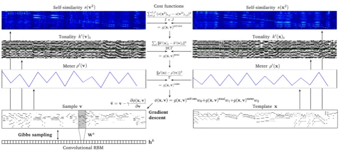
Figure 1: Constrained sampling using an existing piece x as a structure tem-plate. A randomly initialised sample v is alternately updated with Gibbs sampling (GS) and gradient descent (GD). In GD, the error φ(x,y) between structural features of x and v is lowered, in GS the training data distribution is approximated. The Convolutional RBM consists of visible layervand hidden layer h. The filterWk is shared among all units in feature map hk. Depicted equations are also given in Section3.2.
for training instances v, where a ∈ RP and b ∈ RK are bias vectors, and
∗ is the convolution operator. Note that in two-dimensional convolution, each feature map usually has a scalar as bias (e.g. bk), because all positions in a feature map are assumed to be equivalent. However, since we convolve only in the time dimension, and since there is a non-uniform distribution over the pitch dimension, we define the bias for the input feature mapvas a vectoraof length
P.
The probability of a unit being active depends on the full configuration of the opposing layer. When updating hidden unitshand visible unitsv, each unit is randomly chosen to be active (i.e. 1) or inactive (i.e. 0) with probabilities
P(hkj= 1|v) =σ R,P
X
r,p
Wr,pk ×vj×d+r−R
2,p
+bk
(2)
and
P(vtp= 1|h) =σ
R/d,K
X
r,k ˜
Wrk×d,p×hkt+r−R
2d
+ap, (3)
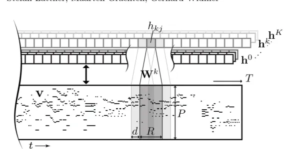
Figure 2: Illustration of a C-RBM with strided convolution (using stride d) in the time dimension t of a music piece v∈RT×P in two-dimensional piano roll
representation using K one-dimensional feature maps hk where all units in a map share their weightsWk∈RR×P and their biasbk (bias not depicted in the illustration).
A sample can be drawn from the model by randomly initialisingv(following thestandard uniform distribution), and running block Gibbs sampling (GS) until convergence. To this end, hidden units and visible units are alternately updated given the other. In doing so, it is common to sample the states of the hidden units for the top-down pass, but use the probabilities of the visible units for the bottom-up pass. After an infinite number of such Gibbs sampling iterations, v
is an accurate sample under the model. In practice, convergence is reached when F(v) stabilises.
The reason for convolving only in the time dimension is that there are correl-ations between notes over the whole pitch range. In a one-layered setting with 2D convolution, the filter height (i.e. the expansion of filters in the pitch dimension) is typically limited, for example, to one octave. In that case, correlations would only be learned between notes within one octave. Learning correlations over a wider range would usually be the role of higher layers in a neural network stack. However, in order to show the principle of constrained sampling it is sufficient to use only one layer with 1D convolution, which is also advantageous for limiting the overall complexity of the architecture.
3.2 Imposing constraints with gradient descent (GD)
When sampling from a C-RBM, the solution is randomly initialised and con-verges to an accurate sample of the data distribution after many steps (see Section 3.1). During this process, we repeatedly adjust the current solution v
using learning rateγ as
ˆ
v=v−γ∂φ(x,v)
∂v , (4)
wherex∈RT×P, 0≤x
tp≤1, is a template piece from which we want to transfer some structural properties to our samplev. After every GD update, we set each entry ˆvtp= min(1,max(0,vˆt,p)), to ensure ˆv∈[0,1]T×P. The cost function may consist of several termsgd(x,v) (weighted with factorswd), each defining a soft constraint which is to be imposed on the sample:
φ(x,v) =g0(x,v)w0+· · ·+gD−1(x,v)wD−1. (5) Note thatxandv, as representations of a musical score, could be assumed to be binary, but we define them ascontinuous variables. This is because we want to store continuous results of the GD optimisation inv, as well as intermediate probabilities during Gibbs sampling. Defining x as a continuous variable is a generalisation towards encoding note intensities or note probabilities, making it possible to express relative importance between notes.
In the following, we will introduce three constraints we tested in our exper-iments. Note that the method is not limited to those constraints, and can be extended with additional terms which are differentiable with respect tov.
Self-similarity constraint The purpose of the self-similarity constraint is to specify the repetition structure (e.g. AABA) in the generated music piece, using a templateself-similarity matrixas a target. Such a self-similarity representation is particularly useful, because it also providesdistances between any two parts of a piece. Thus, the degree of similarity, including strong dissimilarity, may be encoded, too. Such a representation abstracts from the actual musical texture and is therefore to a large extent content-invariant. This allows for transferring the similarity structure in different hierarchical levels between pieces of different style, tonality, or rhythm.
A self-similarity matrixs(z)∈RI×Jfor an arbitrary music piecez∈[0,1]T×P
in piano roll representation is calculated by tilingzhorizontally in tiles of width
Λand by using them as 2-D filters for a convolution over the time dimension of
z(see Fig.3). ThereforeI=T andJ =T /Λ, and we calculate a single entry at positioni, j of the self-similarity matrix as
s(z)i,j= Λ,P
X
λ,p
zj×Λ+λ,pzi+λ,p. (6)
To impose the self-similarity constraint, we minimise the mean squared error (MSE) between a target self-similarity matrix of the squared template piece
s(x2) and the self-similarity matrix of the squared intermediate solutions(v2) as
g(x,v)self-sim=
PI,J
i,j (s(x
2)i,j−s(v2)i,j)2
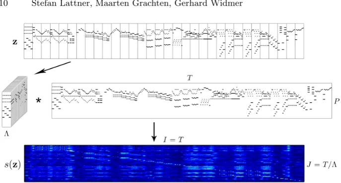
Figure 3: Depiction of calculating the self-similarity matrixs(z)∈RI×J using
convolution. A music piece in piano roll representation z ∈ [0,1]T×P is hori-zontally tiled, and those tiles are used as filters for a convolution with z. The response for a single filter constitutes a single line in the resulting self-similarity matrix. Low to high response is depicted in a range from dark blue to light blue to red.
The reason for squaringxandv is that it leads to a higher stability in the optimisation, because it reduces low intensity noise and it adds contrast to the resulting self-similarity matrix. We also tried to represent transposed repetition as a constraint using two-dimensional convolution. However, we found that this leads to a perfect reconstruction of the template piece, as such a self-similarity representation fully specifies the musical texture.
Tonality constraint Tonality is another very important higher order property in music. It describes perceived tonal relations between notes and chords. This information can be used to, for example, determine thekeyof a piece or a musical section. A key is characterised by a tonal centre (the pitch class that is considered to be central, e.g. C, or A]), and a mode (the subset of pitch classes that form part of the key, e.g. major or minor). The distribution of pitch classes in the musical texture within a (temporal) window of interest is an important factor in the perceived key of that window. Different window lengths M may lead to different key estimates, constituting a hierarchical tonal structure. A common method to estimate the key in a given window is to compare the distribution of pitch classes in the window with so-called key profilesumode (i.e. paradigmatic relative pitch-class strengths for specific modes; the profiles are invariant to changes of tonal centre). In (Temperley,2001), key profiles formajor modeumaj
andminor mode uminare defined as
umin= (5, 2, 3.5, 4.5, 2, 4, 2, 4.5, 3.5, 2, 1.5, 4)>,
where the numerical values express the strengths of the different pitch classes that make up the key. We use these two key profiles as filters for a music piece
z∈[0,1]T×P. By repeating them M times in the time dimension, we obtain a filter for a window of sizeM. By repeating themO =P/12 times in thepitch dimension, we extend the filters over all octaves represented inz. When shifted in the pitch dimension with shifts κ∈0. . .K −1 we obtain a filter for each of theK= 12 possible keys. If we choose the profile for a specific mode umode, an estimation window size M, and the number of octaves O represented byz, we obtain a key estimation vectork(z)modet ∈RK at time tfor all shiftsκas
k(z)modet = M,O,I
X
m,o,i
umode((i+κ) modI)·zt+m,i+o∗12, (8)
forI= 12 entries in key profileuη, where·denotes the common multiplication of scalars. Subsequently, we concatenate the key estimation vectors of both modes,
k(z)majt and k(z)min
t , to obtain a combined estimation vectork(z)t∈R2K in t,
which is finally normalised as
k0(z)t=
k(z)t−min(k(z)t)I
max(k(z)t)−min(k(z)t)
, (9)
whereIis a vector of ones of length 2K.(2) Fig.4depicts the resulting concaten-ated key estimation vectors. Using these vectors, we may impose a specific tonal progression on our solution by minimising the MSE between the target estimate
k0(x)t and the estimate of our current solutionk0(v)tsuch that:
g(x,v)tonal=
P
tkk0(x)t−k0(v)tk2
2KT . (10)
Meter constraint The meter (e.g. 3/4, 4/4, 7/8) defines the duration and the perceived accent patterns in regularly occurring bars of a music piece. For example, in a 4/4 meter, relatively strong accents on the first and the third beat of a bar are common. We impose a common meter extracted from a template piece on our sample, to obtain a degree of global rhythmic coherence.
Perceived accent patterns depend on the relative occurrence of note onsets in a bar, on the intensity of played notes, or on the length of notes starting at the respective positions of a bar. However, note intensities are not encoded in our data, and it is not obvious how to incorporate note durations in our differentiable cost function. Therefore, we use note onsets only. To this end, we constrain the relative occurrence of note onsets within a bar to follow that of a template piece.
(2)Even though the derivatives of min(·) and max(·) are not guaranteed to be always
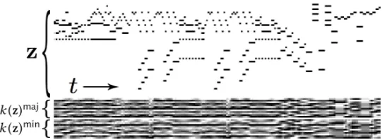
Figure 4: Example of key estimation vectors over time. k(z)maj represent es-timations for 12 possible major keys and k(z)min represent estimations for 12 possible minor keys, where the pitch classes constituting the tonic are ordered from the top to the bottom. Bright pixels represent high strength and dark pixels represent low strength of the respective key. For example, the upper most line in k(z)maj represents the estimation strength of the C major key over time, the third line represents the strength of the D major key, etc.
Abiding by such a distribution helps the generated material to keep implying a regular meter.
The onset functionω(·) results from a discrete differentiation over the time dimension of an arbitrary music piece in piano roll representationz∈[0,1]T×P. We rectify that result (as we are not interested in note offsets), and sum over the pitch dimension:
ω(z, t) = P
X
p
max(0, zt,p−zt−1,p). (11)
In order to calculate the relative occurrences of onsets within a bar, the length T of a bar has to be pre-defined. We count the number of onsets occurring on the respective positions of all bars in the music piece. That is, we sum up all values of distanceT in the onset functionω(·) as
ρ(z)τ = T /T
X
µ
ω(z, τ+µ∗ T), (12)
where τ ∈ 0. . .T −1 is the position in a bar. In our experiments, we use a resolution of 16thnotes in the representation and the template is in 4/4 meter, thereforeT = 16.
To keep the function independent of the absolute number of onsets involved,
ρ(z) is standardised by subtracting its meanρ(z) and dividing through its stand-ard deviationσ(ρ(z)), resulting in zero mean and unit variance:
ρ0(z) = ρ(z)−ρ(z)
Bar position
Relative onset frequency
Relative onset frequencies on bar positions
Figure 5: Relative (standardised) onset frequencies ρ0(z) on bar positions of a music piece as obtained from Equation13.
A standardised onset distribution is plotted in Fig. 5. Finally, we minim-ise the MSE between a standardminim-ised onset distribution ρ0(x) and that of our intermediate solutionρ0(v) as
g(x,v)meter=kρ
0(x)−ρ0(v)k2
T . (14)
4
Constrained Sampling
In this Section, we describe how the C-RBM is used as a generative model to produce musical textures that resemble those of human-composed music, and combined with the soft constraints described above, to enforce additional tonal, meter and self-similarity structure on these textures.
ALGORITHM 1:Constrained Sampling. Number of iterations represent an example scheme, as used in the experiments.
Data:
x∈[0,1]T×P – Template Piece
v∈[0,1]T×P – Random (standard uniform dist.)ˆv=v, N= 250, M = 15
fori∈1. . . N do
v0←v
v←20 GD steps using Eq.4withγ= 10
forj∈1. . . M do
v←100 GS steps usingv
v←1 GD step using Eq.4withγ= 5
end
/* Simulated Annealing */
Ti= 1−i/N
re, rc←random values∈[0,1] if re<exp
−F0(v)−F0(v0)
Ti
orrc<exp
−φ0(x,v)−φ0(x,v0)
Ti
then v←v0
end
/* Store best solution so far */
if F0(v)+2φ0(x,v) <F0(ˆv)+2φ0(x,ˆv) then ˆ
v←v end end return ˆv
4.1 Example scheme and details
In Fig.1, an overview of Constrained Sampling (CS) is shown. During the con-strained sampling process we alternate between a GS phase with the one-layered C-RBM (Section3.1), and a GD optimisation phase on the cost functions (Sec-tion3.2). In each phase, typically multiple iterative updates take place, and the sampling results are sensitive to the balance struck between the GS and GD phases, in terms of the number of updates performed in each phase.
The numbers proposed in the following CS sampling scheme have been found to work well in our experiments. The scheme may have to be adapted to work well with other training settings (e.g. different C-RBM architectures, or different constraints), and is mainly for illustrative purposes. In Algorithm1, the whole process including Simulated Annealing (see Section4.2) is shown.
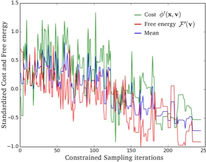
Figure 7: Standardised cost, free energy and their mean in a constrained sampling process over 250 iterations. Periods of constant cost (horizontal line segments) in later iterations are a result of Simulated Annealing, where some unfavourable solution candidates are rejected.
the whole CS process is chosen (see Section 4.2 on standardising the cost and free energy functions).
During CS, in the C-RBM the free energy is to be reduced (i.e. a high prob-ability solution is to be found), while in GD optimisation the objective function is to be minimised (see Fig.7for a plot of the curves). As the two models used compete in approximating their objectives (see Fig. 8), their mutual influence has to be balanced. In addition to using Simulated Annealing to prevent strong deteriorations of the solution with respect to the objectives (see Section 4.2), some parameters need to be carefully adjusted.
The main parameters for balancing the models are the number of GD and GS steps used in a CS iteration, as well as the learning rate and the relative weighting of the cost terms in the GD optimisation (see Tab.1 for weightings used in our experiments). In general, the optimal number of steps in each model is inversely proportional to the size of the training corpus. The more training data, the more possible solutions can be sampled by the probabilistic model making it easier to satisfy constraints imposed by the GD optimisation. Conversely, with a model trained on little data, more GS steps are necessary in order to find another low free energy solution after being distracted by the GD phase.
-20000 -10000 0 10000 20000 30000 40000
0.1 1 10 100 1000 10000
Free energy o
f the C-R
BM
Cost φ(x,v)
Cost vs. Free Energy
GS and GD Only GS Only GD Uniform Noise
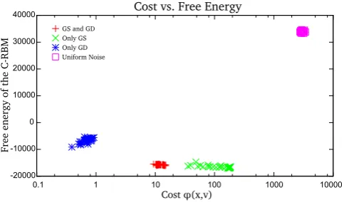
Figure 8: Influence of Gibbs sampling (GS) and gradient descent (GD) on free energyF(v) (see Equation1) and cost φ(x,v) (see Equation5). Using only GS results in low free energy but relatively high cost. Using only GD, the cost is very low but the free energy is high. When using GS and GD, both methods compete, resulting in a trade-off between low cost and low free energy although we choose enough GS steps in the GS phase to always return to a “meaningful”, low free energy state. For reference we test against random uniform noise, resulting in very high free energy and cost. For each cluster, 50 data points were generated with the trained C-RBM model (for GS) and the cost function (for GD) used in our experiment (see Section5)
.
is reached with respect to the overall (average) cost, but not with respect to a final solution in v.
4.2 Simulated Annealing (SA)
Due to the interdependency between the sampling process of the probabilistic model and the GD optimiser, it can easily happen that good intermediate solu-tions deteriorate again by further sampling. Simulated Annealing (SA) helps to find good minima by preventing sampling steps which would lower the solution quality too much (see Algorithm1 for the integration of SA in CS). After each constrained sampling (CS) iteration, we evaluate the SA equation to obtain the probability
pk(v,v0, i) = exp
−f(v)−f(v 0)
Ti
(15)
depicted. In later iterations, Simulated Annealing causes periods of constant cost, as some solution candidates are rejected.
Constraint wd
Self-similarity 1.5 Tonality 5.0
Meter 0.5
Table 1: Relative weightingswd of the terms used in the GD objective function
φ(x,v) (see Section3.2).
5
Experiment
This section describes an experimental validation of the method described in Sections 3 and 4. In Section 5.1 and Section 5.2, we introduce the training data and the data representation scheme, respectively. Section5.3describes the training of the C-RBM. Section 5.4 introduces a quantitative measure for the structural organisation of music, adopted from (Wang & Dubnov,2015). We use this measure to evaluate the success of the constrained sampling approach, both with respect to original musical data, and with respect to other state-of-the-art polyphonic music generation models. Lastly, Section 5.5 briefly describes the procedure followed to produce musical material for qualitative evaluation.
5.1 Training Data
in the training data. Therefore, we transpose each piece into all possible keys, which also helps to reduce sparsity in the training data. This results in a training corpus size of 15144 time steps (of sixteenth note resolution).
A note on training data set size A widely shared insight in machine learning is that to train neural network models effectively, more data is better. In general, it is easy to see why this is the case, since larger amounts of data provide a richer coverage of the relations to be learned in the data. However, depending on the intended purpose of the model, there may be exceptions to this rule. In the present study, where the main purpose of the model is to generate plausible musical textures in the style of Mozart piano sonatas, we have found that the set of all available training data (34 pieces) is likely too small for the C-RBM model to approximate the data distribution well enough to produce samples of high musical quality. A pragmatic trade-off we have chosen in this case is to reduce the size of the training data to a few pieces, and let the model slightly overfit those pieces. This will improve the musical quality of the samples, at the cost of increased local resemblances of generated samples to fragments of the training data.
5.2 Data Representation
We transform MIDI data in a binary piano roll representation of T = 512 time steps over a range of P = 64 pitches (MIDI pitch number 28-92), using a tem-poral resolution of sixteenth notes (see Fig. 6[1a]). Notes are represented by active units (black pixels), and note durations are encoded by activating units up to the note offset. If two notes directly follow each other at the same pitch, they cannot be distinguished any more. Thus, the first note is shortened by a sixteenth note if possible (i.e. if it is longer than a sixteenth note), otherwise the merger has to be accepted. Note that a temporal subdivision of sixteenth notes cannot represent all rhythmic patterns in the data without distortion. For ex-ample, the durations{1/12, 1/12, 1/12}of 1/8 note triplets (as contained in the Sonata No. 1) change to{1/16, 1/8, 1/16}using this representation. We accept this bias, as it does not hinder our efforts to test the influence of constraints on a generated texture.
5.3 Training
We train a single C-RBM using Persistent Contrastive Divergence (PCD) (Tiele-man, 2008) with 10 fantasy particles, using learning rate 15×10−4. Compared to standard Contrastive Divergence (Hinton, Osindero & Teh, 2006), the PCD variant is known to draw better samples. One training instance has a length
Therefore we reset (i.e. randomize) the weights of any neuron which exceeds the threshold of 0.85 average activation over the data.
5.4 Quantitative Evaluation
Based on the observation that probabilistic models can generate meaningful low-level structure but struggle in obeying some higher-low-level structure, the focus of this study is to increase the structural organization of the generated material. In the important case of self-similarity structure, a critical property in music is the balance of repetition and variation. This ratio is expressed by an information theoretic measure called Information Rate (IR). It is the mutual information between the present and the past observations and is maximal when repetition and variation is in balance. Thus, the IR is minimal for random sequences, as well as for very repetitive sequences. It has been shown that it provides a meaningful estimator on musical structure, for instance in parameter selection for musical pattern discovery (Wang & Dubnov,2015).
For a given sequencevN
0 ={v0, v1, v2, . . . , vN}, the average IR is defined by
IR(v0N) = 1
N
N
X
n
H(vn)−H(vn |v0n−1), (16)
where H(v) is the entropy of v, which is estimated based on the statistics of the sequence up to event vn. We approximateH(vn |vn0−1) using a first-order Markov Chain, andH(vn) by counting identical time slices. It may seem counter-intuitive at first sight to utilise a first-order model for measuring the higher-level structure of a piece. Arguably, a low-order estimation yields too optimistic IR values, as the conditional entropy tends to be underestimated. However, the ini-tial idea of contrasting the prior entropy of events with their conditional entropy is still applicable using a first-order entropy estimation. That is, a high IR is achieved when specific events occur rarely, but are very likely given their direct predecessors – a situation which occurs particularly in sequences with higher-level repetition structure. Note that the IR does not provide a measure for the overall musical quality of the evaluated sequences, but only for the aspect of self-similarity structure from an information theoretic point of view.
Information rate
Mozart
Original ConstrainedC-RBM UnconstrainedC-RBM UnconstrainedRNN-RBM UnconstrainedGRU-RBM
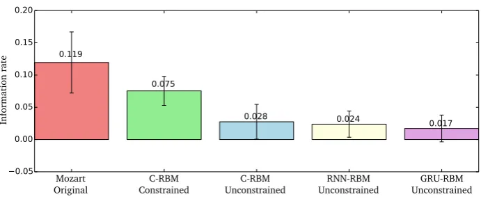
Figure 9: Box plot showing Average Information Rates for 34 original Moz-art piano sonatas, 102 C-RBM samples with structure constraints, 102 C-RBM samples without constraints, 102 samples from an RNN-RBM and 102 samples from a GRU-RBM. Whiskers show standard deviations.
polyphonic music generation model, as a baseline for the quantitative evalu-ation. Furthermore, we replace the RNN portion of the RNN-RBM with Gated Recurrent Units (GRUs, Choet al.,2014) resulting in a GRU-RBM. Both recur-rent models are trained on the same data as the C-RBM, as described in Section
5.1(3).
We compare the average Information Rates between original Mozart piano sonatas (all 34 pieces of the Mozart/Batik data set, Widmer, 2003), C-RBM constrained samples using the original pieces as structure templates (3 samples per original piece resulting in 102 samples with different lengths), 102 C-RBM unconstrained samples, 102 RNN-RBM unconstrained samples and 102 GRU-RBM unconstrained samples. The 102 unconstrained samples per model are created by generating three samples for each original piece of the length of the original piece. For the results of this comparison see Fig.9, for a discussion see Section6.
Further measures for evaluating musical structure Information theory could provide additional quantitative measures for the evaluation of structure in music. An important basis for that is Information Content (IC), a measure of the predictability of an event in a specific context. Prior research has shown that IC can act as a kernel for determining segment boundaries (Pearce, M¨ullensiefen & Wiggins, 2010; Lattner, Grachten, Agres & Chac´on, 2015). Evaluating the plausibility of IC over time in generated sequences could therefore constitute an adequate measure for the evaluation of musical structure.
(3)Samples from the RNN-RBM and the GRU-RBM can be listened to on Soundcloud
window of fixed duration over a musical piece should be constant. For example, Temperley (2014) states “There is a tendency that when an intervallic pattern is repeated with alterations, the alterations tend to lower the probability of the pattern rather than raising it”. When a musical passage is repeated, its Information Content (i.e. the listeners surprise) declines. The finding mentioned above provides some evidence that in such cases, surprising alterations should be inserted to keep the UID constant.
Since the IR is sufficient for evaluating our results, we do not use IC and UID. Nevertheless, they seem promising as further evaluation measures to quantify structure in generated music.
5.5 Qualitative Evaluation
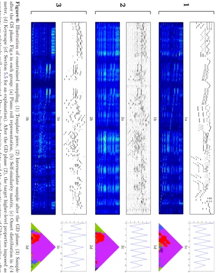
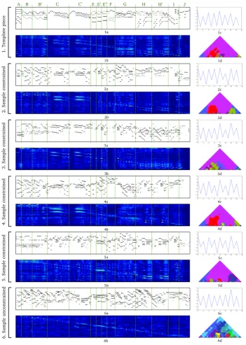
The C-RBM is trained as described in Section 5.3on the Mozart Sonatas (see Section 5.1). After that, we pick a template piece (the first movement of the piano sonata No. 6 in D major) and generate constrained samples, as introduced in Section4. For the weights used to balance the different terms in the GD cost function, see Tab.1. In the self-similarity constraint (see Section3.2), we use a window size Λ of 8 (i.e. half a bar), and for the tonality constraint we use an estimation window widthM of 4 (see Section3.2). Fig.10shows some resulting samples, which are discussed in detail in Section6.
Keyscape We use keyscapes to illustrate the tonality of the pieces in Fig. 6
and Fig.10. A keyscape illustrates the tonal context over a musical piece, where each key receives a distinct colour. We use the humdrum mkeyscape tool by David Huron, which analyses the musical piece with the Krumhansl-Schmuckler key-finding algorithm (Krumhansl, 1990) in different levels of detail. The top of the pyramid depicts the key estimation for the entire piece, while towards the base the analysis is based on ever smaller window sizes. Each scale has a distinct colour assigned to it and the keyscape is coloured according to the most predominant scale estimation.
6
Results and discussion
6.1 Quantitative Evaluation
models without constraints produce music with lower IR than the constrained C-RBM does. Note that the latter point is a non-trivial result, since the self-similarity constraint does not explicitly optimise the Information Rate (neither do the tonal or meter constraints, obviously), but just encourages similarity or dissimilarity between the music at specific positions. This result is in accordance with the initial observation that those models fail to generate higher-level self-similarity structure. Due to their gating mechanism, GRUs are usually better at learning long-term dependencies than regular recurrent units. The fact that the GRU-RBM does not perform better than the RNN-RBM shows that GRUs also have problems in modelling the content-invariant self-similarity property.
6.2 Qualitative Evaluation
Fig.10shows piano roll representations for the template piece (Fig.10[1a]), four generated samples that were constrained with properties from the template piece (Fig.10[2a] to Fig.10[5a]) and a baseline sample generated without constraints from the template piece (Fig. 10[6a]). The corresponding constraints for each musical piece are depicted in the respective figures b-d. The repetition structure is marked on top of the template piece and over all other pieces and self-similarity matrices with vertical, green lines.(4)
We chose the constrained samples by creating 20 solutions and picking the best four with respect to the minimal average value of the standardised GD cost and the standardised free energy over a constrained sampling process (see Section 4.2 on standardising the cost and free energy functions). Thus, results are selected to closely satisfy the given constraints rather than according to their musical quality. Empirically we found that the musical quality in our set-ting increases when loosening the influence of the constraints, as this allows the probabilistic model to create more plausible samples (e.g. the examples in Fig.10sometimes lack appropriate transitions between different sections which is an effect of both constraint satisfaction and limited training data).
By approximating the self-similarity matrix of the template piece, some as-pects of the repetition structure were convincingly transferred to the constrained samples (see Fig.10[1b] to Fig. 10[5b]). For example, the exact repetitions C / C’ and H / H’ occur in every sample. It is interesting to see how the extension of B to B’ is solved. Especially in the samples depicted in Fig.10[2] and Fig.10[3],
(4)All samples illustrated in Fig. 10 can be listened to on Soundcloud under http:
the extension of B is realised by musical textures consistent with the immediate past. In the sample in Fig. 10[5], the model did not produce satisfactory res-ults for phrase B and B’ in a musical sense, although it found a solution which is self-similar over that time period and therefore satisfies that self-similarity constraint to a certain degree.
Parts E / E’ / E” are special cases, because even though they are very similar at first sight, they are transposed repetitions which cannot be captured by the self-similarity matrix as it is currently defined. In the self-similarity matrix of the template, we see that each of those “E” sections is more or less similar or dis-similar to different regions in the piece. In addition, we note that each repetition has the length of one bar. When comparing these “E” sections with those in the samples, we recognise the limits of the method concerning temporal resolution. The C-RBM has a filter length of one bar, which is too wide for sampling three bars with different requirements concerning similarity, while keeping a plausible low-level structure. Therefore, in some samples the generated patterns span the whole, or at least two of the “E” sections.
Part G in the repetition structure is similar to most parts of the piece, as can be seen from the bright areas over the full height of the respective self-similarity matrices. In the samples this is realised by choosing textures which are also similar to most parts. Part J, in contrast, is very dissimilar to most areas of the template piece. Probably due to limited training data, this sometimes results in empty areas in the samples. Except for an apparent similarity in B and B’, which is not reflected in the self-similarity matrix, the unconstrained baseline sample does not follow the repetition structure of the template piece.
The onset distributions (see Subplotscin Fig.10), which are plots resulting from Equation 13, are sometimes rather dissimilar to the onset distribution of the template. This shows that it is not easy to approximate this global property. One reason for this may be that it is a property which summarises the complete music piece in only a few values, which makes it easy in the GD optimisation to approximate by distributing small changes over the whole sample. Those are, however, locally not strong enough to be kept during GS. Incorporating note durations for emphasizing onsets of longer notes would lead to more character-istic onset distributions, which could further lead to bigger local changes in the probability of notes in the piano roll. However, in the onset distributions there is a tendency of the peaks at position 0 and 8 to be higher than the others, which corresponds to the tendency in the onset distribution of the template piece. Note that the reason for every second value in the distributions being low is not the meter constraint but the stride of one beat in the convolution. This provides the model with a regular grid allowing it to learn that the probability of an onset is lower at every second time step. Therefore, those values are also low for the unconstrained baseline piece.
indicates tonal incoherence.
As mentioned above, the illustrated samples are the best four of 20 with respect to the overall cost. The most obvious shortcoming of samples not selected because of higher cost is that they do not satisfy some of the given structural constraints on a local level. This includes the failure to reproduce a repetition at specific positions, or erroneously modulating into a key which does not occur in the template piece. However, a closer inspection of such cases shows that incorrect keys are often closely related to the desired keys, for instance the parallel minor/major key. Parallel minor/major keys have most of their pitches in common, but they are expected to follow a different distribution. Another common problem in the non-optimal samples is that they show areas without any notes, which is probably a symptom of the contrasting objectives of GD and GS. We found that the C-RBM is very sensitive to changes in the parameters of the whole system. Other models able to perform GS could lead to a more stable functioning, like LSTMs used for GS in (Hadjereset al.,2017).
7
Conclusion and future work
Music is typically highly structured at both lower and higher levels. State-of-the-art sequence models such as RNNs and LSTMs have been successfully used to generate music in restricted settings, but in more complex musical mater-ial, such as piano music from the classical or romantic period, not to mention orchestral works, important musical characteristics such as tonal, metrical and self-similarity structure tend to defy straight-forward time series modelling ap-proaches.
The constrained sampling method for music generation presented here ad-dresses this problem by combining a stochastic neural network for sampling plausible musical textures at a local level with soft constraints that impose higher-level structure regarding meter, tonality and self-similarity structure, ob-tained from a template piece.
The empirical results also reveal some shortcomings. Firstly, while imposing constraints with the proposed method helps to generate high-level structure, meaningful low-level structure can currently only be generated when the model is trained on relatively small amounts of data. Overcoming this drawback may require more powerful generative models – amenable to some form of Gibbs sampling – as an alternative to the C-RBM. Our hypothesis is that generative models can only generalise well on low-level structure if they are able to explicitly represent (transposed) repetition. A promising approach to this is proposed by Lattner and Grachten (2017), who show that relations between musical sections can be learned and represented as so-called “mapping codes”.
Secondly, when listening to the generated musical samples it is clear that the tonal, meter and self-similarity constraints presented here are by no means fully elaborated nor exhaustive. For example, more specialised constraints – like a differentiable formalisation of the IR measure – could optimise sequences to directly obey desired structural properties. Perhaps most importantly, what is currently missing is a constraint that enforces musical closure at boundaries of structural units. Without such a constraint, the music contains repeated musical structures, but these structures are hard to identify perceptually because their boundaries are not marked by salient musical cues (such as harmonic resolution). That said, the proposed constrained sampling approach is general enough to accommodate this and possibly other constraints.
Acknowledgements This research was supported by the EU FP7 (project Lrn2Cre8, FET grant number 610859), and the European Research Council (pro-ject CON ESPRESSIONE, ERC grant number 670035).
References
Aylett, M. & Turk, A. (2006). Language redundancy predicts syllabic duration and the spectral characteristics of vocalic syllable nuclei.The Journal of the Acoustical Society of America, 119(5), 3048–3058. doi:10.1121/1.2188331
Barbieri, N. (2011). Regularized gibbs sampling for user profiling with soft con-straints. In International conference on advances in social networks ana-lysis and mining, ASONAM 2011, Kaohsiung, Taiwan, 25-27 July 2011 (pp. 129–136). IEEE Computer Society. doi:10.1109/ASONAM.2011.92
Choi, K., Fazekas, G. & Sandler, M. B. (2016). Text-based LSTM networks for automatic music composition.CoRR,abs/1604.05358. arXiv:1604.05358. Retrieved fromhttp://arxiv.org/abs/1604.05358
Collins, T., Laney, R. C., Willis, A. & Garthwaite, P. H. (2016). Developing and evaluating computational models of musical style. Artificial Intelligence for Engineering Design, Analysis and Manufacturing,30(1), 16–43. doi:10. 1017/S0890060414000687
Conklin, D. (2016). Chord sequence generation with semiotic patterns.Journal of Mathematics and Music, 10(2), 92–106. doi:10 . 1080 / 17459737 . 2016 . 1188172. eprint:https://doi.org/10.1080/17459737.2016.1188172
Cope, D. (1996). Experiments in musical intelligence. (Vol. 12). Madison, WI: AR editions.
Eck, D. & Schmidhuber, J. (2002).A first look at music composition using LSTM recurrent neural networks. Istituto Dalle Molle Di Studi Sull Intelligenza Artificiale. Retrieved fromwww.iro.umontreal.ca/∼
eckdoug/blues/IDSIA-07-02.pdf
Eigenfeldt, A. & Pasquier, P. (2013). Evolving structures for electronic dance mu-sic. InGenetic and evolutionary computation conference, GECCO ’13, Am-sterdam, The Netherlands, July 6-10, 2013 (pp. 319–326). ACM. doi:10. 1145/2463372.2463415
Gatys, L. A., Ecker, A. S. & Bethge, M. (2016). Image style transfer using convo-lutional neural networks. In2016 IEEE conference on computer vision and pattern recognition, CVPR 2016, Las Vegas, NV, USA, June 27-30, 2016 (pp. 2414–2423). IEEE Computer Society. doi:10.1109/CVPR.2016.265
Graves, A. (2013). Generating sequences with recurrent neural networks.CoRR, abs/1308.0850. arXiv: 1308.0850. Retrieved from http://arxiv.org/abs/ 1308.0850
Hadjeres, G., Pachet, F. & Nielsen, F. (2017). DeepBach: A steerable model for bach chorales generation. In D. Precup & Y. W. Teh (Eds.), Pro-ceedings of the 34th international conference on machine learning, ICML 2017, Sydney, NSW, Australia, August 6-11, 2017 (Vol. 70, pp. 1362– 1371). Proceedings of Machine Learning Research. PMLR. Retrieved from
http://proceedings.mlr.press/v70/hadjeres17a.html
Hinton, G. E., Osindero, S. & Teh, Y. (2006). A fast learning algorithm for deep belief nets.Neural Computation,18, 1527–1554.
Huang, C. A., Cooijmans, T., Roberts, A., Courville, A. C. & Eck, D. (2017). Counterpoint by convolution. In S. J. Cunningham, Z. Duan, X. Hu & D. Turnbull (Eds.),Proceedings of the 18th international society for music information retrieval conference, ISMIR 2017, Suzhou, China, October 23-27, 2017(pp. 211–218). Retrieved from https://ismir2017.smcnus.org/wp-content/uploads/2017/10/187 Paper.pdf
Jordanous, A. (2012). A standardised procedure for evaluating creative systems: Computational creativity evaluation based on what it is to be creative. Cognitive Computation,4(3), 246–279. doi:10.1007/s12559-012-9156-1
Kirchmeyer, H. (1968). On the historical constitution of a rationalistic music. (Vol. 8, pp. 11–24). Die Reihe.
Krumhansl, C. L. (1990). Cognitive foundations of musical pitch. (Vol. 17, pp. 77– 110). Oxford Psychology Series. New York: Oxford University Press. Lattner, S. & Grachten, M. (2017). Learning transformations of musical material
using gated autoencoders. In Proceedings of the 2nd conference on com-puter simulation of musical creativity, CSMC 2017, Milton Keynes, UK, September 11-13, 2017. Retrieved from https://drive.google.com/open? id=0B12H6lLCqzLWdVgwMFZON25UM3c
Lattner, S., Grachten, M., Agres, K. & Chac´on, C. E. C. (2015). Probabilistic segmentation of musical sequences using restricted Boltzmann machines. In T. Collins, D. Meredith & A. Volk (Eds.), Proceedings of the 5th in-ternational conference on mathematics and computation in music, MCM 2015, London, UK, June 22-25, 2015 (Vol. 9110, pp. 323–334). Lecture Notes in Computer Science. Springer. doi:10.1007/978-3-319-20603-5 33
LeCun, Y., Boser, B. E., Denker, J. S., Henderson, D., Howard, R. E., Hubbard, W. E. & Jackel, L. D. (1989). Backpropagation applied to handwritten zip code recognition.Neural Computation, 1(4), 541–551. doi:10.1162/neco. 1989.1.4.541
Lee, H., Ekanadham, C. & Ng, A. Y. (2007). Sparse deep belief net model for visual area V2. In J. C. Platt, D. Koller, Y. Singer & S. T. Roweis (Eds.), Proceedings of the twenty-first annual conference on neural information processing systems, Vancouver, British Columbia, Canada, December 3-6, 2007(pp. 873–880). Curran Associates, Inc. Retrieved fromhttp://papers. nips.cc/paper/3313-sparse-deep-belief-net-model-for-visual-area-v2
Lee, H., Grosse, R. B., Ranganath, R. & Ng, A. Y. (2009). Convolutional deep belief networks for scalable unsupervised learning of hierarchical represent-ations. In A. P. Danyluk, L. Bottou & M. L. Littman (Eds.),Proceedings of the 26th annual international conference on machine learning, ICML 2009, Montreal, Quebec, Canada, June 14-18, 2009 (Vol. 382, pp. 609– 616). ACM International Conference Proceeding Series. ACM. doi:10.1145/ 1553374.1553453
national society for music information retrieval conference, ISMIR 2017, Suzhou, China, October 23-27, 2017 (pp. 449–456). Retrieved fromhttps: //ismir2017.smcnus.org/wp-content/uploads/2017/10/156 Paper.pdf
Lyu, Q., Wu, Z., Zhu, J. & Meng, H. (2015). Modelling high-dimensional se-quences with LSTM-RTRBM: Application to polyphonic music generation. In Q. Yang & M. Wooldridge (Eds.),Proceedings of the twenty-fourth in-ternational joint conference on artificial intelligence, IJCAI 2015, Buenos Aires, Argentina, July 25-31, 2015 (pp. 4138–4139). AAAI Press. Re-trieved fromhttp://ijcai.org/Abstract/15/582
Mozer, M. C. (1994). Neural network music composition by prediction: Explor-ing the benefits of psychoacoustic constraints and multi-scale processExplor-ing. Connect. Sci. 6(2-3), 247–280. doi:10.1080/09540099408915726
Pachet, F. & Roy, P. (2011). Markov constraints: Steerable generation of Markov sequences.Constraints,16(2), 148–172. doi:10.1007/s10601-010-9101-4
Palmer, C. & Krumhansl, C. L. (1990). Mental representations for musical meter. Journal of Experimental Psychology: Human Perception and Performance, 16(4), 728–741.
Pearce, M., M¨ullensiefen, D. & Wiggins, G. A. (2010). The role of expectation and probabilistic learning in auditory boundary perception: a model com-parison.Perception,39(10), 1365–1389. doi:10.1068/p6507
Pearce, M. & Wiggins, G. (2001). Towards a framework for the evaluation of machine compositions. InProceedings of the symposium on artificial intel-ligence and creativity in the arts and sciences, AISB’01, York, UK, March 21-24, 2001 (pp. 22–32). AISB Press.
Roberts, A., Engel, J. & Eck, D. (2017). Hierarchical variational autoencoders for music. InNIPS workshop on machine learning for creativity and design, Long Beach, California, USA, December 8, 2017.
Shannon, C. E. (1948). A mathematical theory of communication. Bell System Technical Journal, 27, 379–423, 623–656. Retrieved from http : / / math . harvard.edu/∼ctm/home/text/others/shannon/entropy/entropy.pdf Smith, N. A. & Schmuckler, M. A. (2004). The perception of tonal structure
pp. 545–560). Lecture Notes in Computer Science. Springer. doi:10.1007/ 11503415 37
Sturm, B., Santos, J. F., Ben-Tal, O. & Korshunova, I. (2016). Music transcrip-tion modelling and compositranscrip-tion using deep learning. InProceedings of the 1st conference on computer simulation of musical creativity. Huddersfield, UK. Retrieved fromhttps://goo.gl/uEzGeQ
Taylor, G. W., Hinton, G. E. & Roweis, S. T. (2006). Modeling human mo-tion using binary latent variables. In B. Sch¨olkopf, J. C. Platt & T. Hof-mann (Eds.),Advances in neural information processing systems 19, ceedings of the twentieth annual conference on neural information pro-cessing systems, Vancouver, British Columbia, Canada, December 4-7, 2006 (pp. 1345–1352). MIT Press. Retrieved from http : / / papers . nips . cc/paper/3078-modeling-human-motion-using-binary-latent-variables
Temperley, D. (2001). The cognition of basic musical structures. Cambridge, Mass.: MIT Press.
Temperley, D. (2014). Information flow and repetition in music.Journal of Music Theory,58(2), 155–178. doi:10.1215/00222909-2781759
Theano Development Team. (2016). Theano: A python framework for fast com-putation of mathematical expressions.CoRR,abs/1605.02688. arXiv:1605. 02688. Retrieved fromhttp://arxiv.org/abs/1605.02688
Tieleman, T. (2008). Training restricted Boltzmann machines using approxima-tions to the likelihood gradient. In W. W. Cohen, A. McCallum & S. T. Ro-weis (Eds.),Machine learning, proceedings of the twenty-fifth international conference (ICML 2008), Helsinki, Finland, June 5-9, 2008 (Vol. 307, pp. 1064–1071). ACM International Conference Proceeding Series. ACM. doi:10.1145/1390156.1390290
Todd, P. M. (1989). A connectionist approach to algorithmic composition. Com-puter Music Journal,13(4), 27. doi:10.2307/3679551
Wang, C. & Dubnov, S. (2015). Pattern discovery from audio recordings by vari-able Markov oracle: A music information dynamics approach. In Proceed-ings of the IEEE international conference on acoustics, speech and signal processing, ICASSP 2015, South Brisbane, Queensland, Australia, April 19-24, 2015 (pp. 683–687). IEEE. doi:10.1109/ICASSP.2015.7178056
Whorley, R. & Conklin, D. (2016). A transformational method for chorale gener-ation. InProceedings of the 9th international workshop on machine learning and music, MML 2016, Riva del Garda, Italy, September 23, 2016(pp. 71– 75). Retrieved fromhttp://www.ehu.eus/cs-ikerbasque/conklin/papers/ rw16mml.pdf