Online Learning for Statistical Machine Translation

Machine Translation

Daniel Ortiz-Mart´ınez

Universitat Polit`ecnica de Val`encia1

We present online learning techniques for statistical machine translation (SMT). The availability of large training data sets that grow constantly over time is becoming more and more frequent in the field of SMT—for example, in the context of translation agencies or the daily translation of government proceedings. When new knowledge is to be incorporated in the SMT models, the use of batch learning techniques require very time-consuming estimation processes over the whole training set that may take days or weeks to be executed. By means of the application of online learning, new training samples can be processed individually in real time. For this purpose, we define a state-of-the-art SMT model composed of a set of submodels, as well as a set of incremental update rules for each of these submodels. To test our techniques, we have studied two well-known SMT applications that can be used in translation agencies: post-editing and interactive machine translation. In both scenarios, the SMT system collaborates with the user to generate high-quality translations. These user-validated translations can be used to extend the SMT models by means of online learning. Empirical results in the two scenarios under consideration show the great impact of frequent updates in the system performance. The time cost of such updates was also measured, comparing the efficiency of a batch learning SMT system with that of an online learning system, showing that online learning is able to work in real time whereas the time cost of batch retraining soon becomes infeasible. Empirical results also showed that the performance of online learning is comparable to that of batch learning. Moreover, the proposed techniques were able to learn from previously estimated models or from scratch. We also propose two new measures to predict the effectiveness of online learning in SMT tasks. The translation system with online learning capabilities presented here is implemented in the open-source Thot toolkit for SMT.

1 The author is now at Webinterpret.

1. Introduction

Multiplicity of languages is inherent to modern society. Phenomena such as global-ization and technological development have extraordinarily increased the need for translating information from one language to another. One possibility to deal with this growing demand of translations is the use of machine translation (MT) techniques.

∗PRHLT Research Center, Universitat Polit`ecnica de Val`encia, 46071, Val`encia, Spain, E-mail:[email protected].

Submission received: 2 May 2014; revised version received: 2 October 2015; accepted for publication: 20 November 2015.

MT can be formalized under a statistical point of view as the process of finding the sentence of maximum probability in the target language given the source sentence. Statistical MT (SMT) requires the availability of parallel texts to estimate the statistical models involved in the translation. It is also important that such parallel texts belong to the same domain the system will be used for. These kinds of texts are referred to as in-domaincorpora in the domain adaptation literature. However, in-domain corpora are often not available in real translation scenarios, forcing us to estimate the system models by means of large out-of-domain texts, such as Parliament proceedings. Unfortunately, this results in a significant degradation in the translation quality (Irvine et al. 2013).

There are many real translation scenarios in which new training data is inherently generated over time (e.g., translation agencies or the daily translation of government proceedings). The newly generated training data could be used to mitigate the problem of data scarcity. However, this situation poses new challenges in the SMT framework, because the vast majority of the SMT systems described in the literature makes use of the well-knownbatch learning paradigm. In the batch learning paradigm, the train-ing of the SMT system and the translation process are carried out in separate stages. This implies that all training samples must be available before training takes place, preventing the statistical models to be extended when the system starts generating translations. To solve this problem, theonline learningparadigm can be applied. Online learning is a machine learning task that is structured in a series of trials, where each trial has four steps: (1) the learning algorithm receives an instance, (2) a label for the instance is predicted, (3) the true label for the instance is presented, and (4) the learning algorithm uses the true label to update its parameters. In this paradigm, the training and prediction stages are no longer separated.

Online learning fits nicely in typical computer-assisted translation (CAT) appli-cations used in translation agencies. This is because in such appliappli-cations the system translation for each source sentence is validated by a human expert and thus can be used to produce new training pairs. One possible CAT implementation consists of post-editing (PE) the output of an MT system. In this implementation, the MT system generates an initial translation that is corrected by the user without further system intervention. Another instance of CAT is interactive machine translation (IMT), where the user generates each translation in a series of interactions with the system.

Scientific and commercial interest in CAT applications has greatly increased dur-ing recent years, capturdur-ing the attention of internationally renowned research groups and translation companies. A good example of this is the work carried out in the TransType (Foster, Isabelle, and Plamondon 1997) and TransType-II (SchlumbergerSema S.A. et al. 2001) research projects, where the IMT paradigm was developed, and the CasMaCat (Alabau et al. 2014) and MateCat (Federico et al. 2014) projects, where a substantial part of the effort was focused on developing adaptive learning techniques for CAT. Literature also offers demonstrations of CAT applications (Koehn 2009; Ortiz-Mart´ınez et al. 2011) as well as studies involving real users showing the potential benefits of CAT (Green, Heer, and Manning 2013; Ortiz-Mart´ınez et al. 2015).

new blocks of training data obtained from different sources, such as parliamentary proceedings.

The rest of the article is organized as follows: Section 2 describes the statistical foundations of SMT and its adaptation to the PE and IMT scenarios. Section 3 explains the online learning techniques proposed here, including the definition of a log-linear SMT model as well as a set of incremental update rules for each one of its components. The content of Section 3 is complemented by Appendix A, which presents an alternative incremental update rule for word-alignment models. Experimental results as well as their discussion are shown in Sections 4 and 5, respectively. Section 6 describes related work on online learning. The work conclusions are given in Section 7.

2. Statistical Framework

In this section we describe the details of the statistical framework adopted in the rest of the article. For this purpose, we briefly describe the statistical formulation of SMT as well as the required modifications for its use in two well-known applications of SMT, namely, post editing and interactive machine translation.

2.1 Statistical Machine Translation

In the statistical approach to MT, given a source sentencef₁J≡f1...fj...fJ in the source languageF, we want to find its equivalent target sentenceeI₁≡e1...ei...eIin the target languageE, wherefjandeinote theith word and thejth word of the sentencesf₁Jand

eI

1, respectively. From the set of all possible sentences of the target language, we are interested in that with the highest probability according to the following equation:

ˆ

eI₁ˆ=arg max I,eI

1

{Pr(eI₁|f₁J)} (1)

Early works on SMT decomposePr(eI₁|f₁J) applying Bayes’ theorem and thus ob-taining two new distributions,Pr(eI₁) andPr(f₁J|eI₁), which are approximated by means of parametric statistical models. Specifically,Pr(eI₁) is modeled by means of alanguage model, andPr(f₁J|eI

1) is modeled by means of atranslation model.

Statistical language models are typically implemented with n-gram language models. Regarding the translation models, they are commonly implemented using the so-calledphrase-based models(Koehn, Och, and Marcu 2003). The basic idea of phrase-based translation is to segment the source sentence into phrases, then to translate each source phrase into a target phrase, and finally to reorder the translated target phrases in order to compose the target sentence. The decisions made during the phrase-based translation process can be summarized by means of the hidden variable ˜aK₁ ≡a˜1...a˜k...a˜K, where ˜ak denotes the index of the target phrase ˜ek that is aligned with thekth source phrase ˜fk, determining abisegmentationof the source and target sentences of lengthK. Alternative formalizations to the one using Bayes’ theorem have been proposed. Such formalizations are based on the direct modeling of the posterior probability,

Pr(eI 1|f

J

are strongly focused on these phrase-based models, obtaining the best alignment at phrase level:

ˆ

eI₁ˆ=arg max I,eI

1

max K,˜aK

1

R

X

r=1

λ_rhr(f1J,eI1, ˜aK1)

(2)

where a total ofRfeature functions are assumed.

State-of-the-art decoders work by exploring the search space determined by Equa-tion (2) using iterative algorithms that build partial target translaEqua-tions from left to right.

2.2 Post-Editing the Output of Statistical Machine Translation

Post-editing (PE) involves making corrections to machine generated translations (see TAUS-Project [2010] for a detailed study). PE is used when raw machine translation is not error-free, a common situation for current MT technology. PE tends to be carried out via tools built for editing human-generated translations, such as translation mem-ories (some authors refer to this task as simply editing). Because in the PE scenario, the user only edits the output of the MT system without further intervention from the system, there are no differences in the way in which the MT system is designed and implemented. Hence, the statistical framework for MT described previously can be adopted without modifications in order to build the PE system.

2.3 Statistical Interactive Machine Translation

One alternative to the serial collaboration model adopted by PE is interactively com-bining the MT system with a human translator, constituting the interactive machine translation (IMT) paradigm (also referred to as interactive translation prediction). One possible IMT implementation uses SMT systems to produce target sentence hypotheses that can be partially or completely accepted and amended by a human translator (Barrachina et al. 2009). Each partially corrected text segment, or prefix, is then used by the SMT system as additional information to achieve improved suggestions.

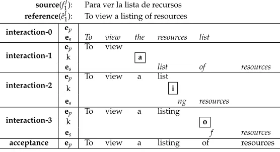
Figure 1 illustrates a typical IMT session. In interaction-0, the system suggests a complete translation hypothesis,es, given the source sentence,f1J. In interaction-1, the user moves the mouse to accept the prefix composed of the first eight charactersTo view

(that is, the prefix of the sentence the user deems to be correct) and presses the a key (k), producing the prefix,ep. Then the system suggests completing the sentence withlist

of resources(a newes), given the accepted and correct prefix. Interactions-2 and -3 are similar. In the final interaction, the user accepts the current translation suggestion.

In the IMT scenario we have to find an extensionesfor a user prefixep:2

ˆ

es=arg max

es

{p(es|f1J,ep)} (3)

If Bayes’ theorem is applied, we then obtain two distributions, p(es|ep) and

p(f₁J|ep,es), that are very similar to those obtained for conventional SMT, sinceepes≡

eI₁. This allows us to use the same models if the search procedures are adequately

source(f₁J): Para ver la lista de recursos reference(ˆeI₁): To view a listing of resources interaction-0 ep

es To view the resources list interaction-1

ep To view

k a

es list of resources interaction-2

ep To view a list

k listi

es listing resources

interaction-3

ep To view a listing

k o

es of resources

acceptance ep To view a listing of resources

Figure 1

An example of an IMT session to translate a Spanish sentence into English.

modified. Specifically, the search is restricted to generate target sentences compatible with the user prefix.3 Note that the statistical models are defined at the word level whereas the IMT interface described in Figure 1 works at the character level. This is not an important issue because the transformations that are required in the statistical models for their use at character level are trivial. Specifically, the compatibility with the user prefix is verified by comparing characters instead of words.

3. Online Learning for Statistical Machine Translation

In this section we describe the concept of online learning and its application to SMT.

3.1 Definition of Online Learning

Online learning algorithms proceed in a sequence of trials. Each trial can be decomposed into four steps:

1. The learning algorithm receives an instance.

2. The learning algorithm predicts a label for the instance according to its current parameters.

3. The true label of the instance is presented to the learning algorithm.

4. The learning algorithm uses the true label to update its parameters.

The system uses the true label to measure the prediction error incurred by the learner and discarded afterwards. The ultimate goal of the online learning algorithm is to minimize the cumulative prediction error along its run by modifying its parameters.

More formally, given any sequence of training samplesx1,x2,..., an online learning algorithm produces a sequence of parameters:Θ(0),Θ(1),Θ(2),..., such that the algorithm parameters at trialt, Θ(t), depends only on the previous parameters, Θ(t−1), and the current samplext.

One important consequence of discarding the training samples after each trial is that the computational complexity of processing a new sample does not depend on the number of samples that has been previously seen. That is, the computational complexity of processing a new sample is constant.

The online learning algorithms that discard each new training sample after up-dating the learner are also referred to as incremental learning algorithms by some authors (see Anthony and Biggs [1992]). However, this constraint can be relaxed by using mini-batches (small sets of samples).

The online learning setting contrasts with the batch learning setting, in which all the training patterns are presented to the learner before learning takes place and the learner is no longer updated after the learning stage has concluded.

Batch learning algorithms are appropriate for their use in stationary environments. In a stationary environment, all instances are drawn from the same underlying proba-bility distribution. By contrast, because online learning algorithms continually receive prediction feedback, they can be used in non-stationary environments.

The design of online learning algorithms raises issues not present in batch learning settings. Three of them are identified in Giraud-Carrier (2000): (1)Chronology: the order in which knowledge is acquired is an inherent aspect of online learning, (2)Learning curve: the learner may start from scratch and gain knowledge from examples given one at a time over time; as a result, it experiences a sort of learning curve, and (3)Open-world assumption: all the data relevant to the problem at hand is not available a priori.

Finally, online learning is also related to another learning paradigm: active learn-ing. In this paradigm the system queries the user to obtain the true labels of specific instances, obtaining greater accuracy using less training data. Active learning can also be applied in online settings, where the capability of the system to learn in an online or incremental manner using techniques like those proposed here is crucial. One example of this is the work presented in Gonz´alez-Rubio, Ortiz-Mart´ınez, and Casacuberta (2012), where active learning techniques for IMT are proposed.

3.2 Implementing Online Learning

The key aspect to be considered when implementing online learning algorithms is how to update the system parameters given the previous ones and the new training sample. If the online learning algorithm is based on statistical models, then we need to maintain a set of sufficient statistics for these models that can be incrementally updated. A sufficient statistic for a statistical model is a statistic that captures all the information that is relevant to estimate this model. If the estimation of the statistical model does not require the use of the expectation–maximization (EM) algorithm (e.g.n-gram language models), then it is generally easy to incrementally extend the model given a new training sample. By contrast, if the EM algorithm is required (e.g., word alignment models), the estimation procedure has to be modified, since conventional EM is designed for its use in batch learning scenarios. To solve this problem, an incremental version of the EM algorithm is required.

3.3 Predicting the Effectiveness of Online Learning in SMT Tasks

now able to efficiently learn translations for new or previously seen words. However, the benefits will only be significant when the document to be translated presents a high internal repetition rate, since this will allow the system to take advantage of the newly acquired knowledge. This should not be seen as a limitation specific to online learning. In batch learning scenarios the translation quality is strongly weakened if the training corpus is not representative of the text to be translated. When we move to an online setting, we still have the same requirement but now the training and translation stages are no longer separated. This is why we speak about repetitiveness instead of representativeness. In any case, sufficiently high repetition rates for test doc-uments are common, according to the document-internal repetition property defined in Church and Gale (1995).

Bertoldi, Cettolo, and Federico (2013) propose an automatic measure for assessing the potential usefulness of online learning: the repetition rate (RR). In this section we will slightly modify the definition of RR and propose two additional measures.

The RR measure looks at the rate of non-singleton n-grams contained in a given text. More specifically, the rates of non-singletonn-grams fromn=1 to 4 are calculated and geometrically averaged, using a sliding window of 1, 000 words to make the rates comparable across different sized corpora. Here we use a slightly modified version in which the sliding window calculation is removed, because in real translation scenarios the text to be translated is available beforehand and should be completely translated. Thus, we define our modified RR (MRR) measure as follows:

MRR(I)= 4

Y

n=1

|I_n,1+| − |In,1|

|I_n,1+|

!1/4

(4)

where | · | represents the length of a given set, I_n,1+ represents the set of different

n-grams contained in the in-domain corpusI, andI_n,1 represents the set of different

n-grams occurring only once inI.

The MRR measure does not take into account whether a specificn-gram is contained or not in the out-of-domain corpus that has been used to estimate the SMT models. According to Irvine et al. (2013), unseen events constitute a major cause of translation errors when migrating an existing SMT system to a new domain. Thus, it is interesting to restrict the calculation of the repetition rate to thosen-grams that are not contained in the out-of-domain corpus. We will refer to this measure as therestricted repetition rate(RRR):

RRR(I,O)= 4

Y

n=1

|I_n,1+−O_n,1+| − |I_n,1−O_n,1+| |I_n,1+−On,1+|

!1/4

(5)

where O_n,1+ represents the set of different n-grams contained in the out-of-domain

corpusO.

if the fraction of unseenn-grams is very low. To capture this corpus property, we define theunseenn-gram fraction(UNF) measure:

UNF(I,O)=



 

4

Y

n=1

P

w∈(In,1+−On,1+)

cI(w)

P

w∈In,1+

cI(w) 

 

1/4

(6)

wherecI(w) represents the count ofn-gramwin corpusI.

Here we propose to predict the potential usefulness of online learning, paying attention only to the RRR and the UNF measures. In spite of this, MRR will be also reported so as to compare the information provided by the three measures.

3.4 Statistical Phrase-Based Log-Linear Model for Online SMT

As stated in Section 2.1, log-linear models including phrase-based models as feature functions constitute the state-of-the-art in statistical machine translation. In this section we will describe the components of our log-linear model for SMT. Later, in Section 3.5, the update rules required to extend such components will be presented.

According to Equation (2), we introduce a set of seven feature functions in our log-linear model: an n-gram language model (h1), a source sentence-length model (h2), inverse and direct phrase-based models (h3 and h4, respectively), a tar-get phrase-length model (h5), a source phrase-length model (h6), and a distortion (or phrase reordering) model (h7). All these feature functions, with the exception of the one related to the direct phrase-based model (h4), can be obtained from a proper decomposition of the distribution Pr(eI

1|f J

1) (the decomposition is detailed in Ortiz-Mart´ınez [2011]).

This set of feature functions is similar to those incorporated into other state-of-the-art SMT systems such as the Moses decoder (Koehn et al. 2007). The main difference of our proposal with existing works is that we have paid special attention to the formal justification of the features.

We next list the details for each feature function.

r

h1(eI1)=log I+1

Y

i=1

p(ei|eii−−1n+1)

!

4Iis the length ofeI₁,e0is thebegin-of-sentencesymbol,e|e|+1is theend-of-sentencesymbol,e

wherep(ei|eii−−1n+1) is defined as follows:

p(ei|eii−−1n+1)=

max{cX(eii−n+1)−Dn, 0}

cX(ei_i−−1n+1)

+

Dn

cX(eii−−1n+1)

N1+(ei_i−−1n+1•)·p(ei|e i−1

i−n+2) (7)

whereDn= cn,1cn+,12cn,2 is a fixed discount (cn,1andcn,2are the number ofn-grams with

one and two counts respectively),N1+(ei_i−−1n+1•) is the number of unique words that follows the history ei_i−₋1_n+1, andcX(eii−n+1) is the count of the n-grameii−n+1, where

cX(·) can represent true countscT(·) or modified countscM(·).

True counts are used for the higher ordern-grams and modified counts for the lower order n-grams. Given a certain n-gram, its modified count consists of the number of different words that precede thisn-gram in the training corpus.

Equation (7) corresponds to the probability given by ann-gram language model with an interpolated version of the Kneser-Ney smoothing (Chen and Goodman 1996).

r

h2(f1J,e1I)=log(p(J|I))=log(φI(J+0.5)−φI(J−0.5))

where φ_I(·) is the cumulative distribution function for the normal distribution (the cumulative distribution function is used to integrate the normal density function over an interval of length 1). A specific target sentence length Iwill be assigned during decoding time when a new empty hypothesis is created. After that, this hypothesis will be extended in successive trials, but it will be constrained to haveIwords when all the source words are covered. The sentence length model is introduced to avoid the generation of too short or too long target sentences, which negatively impact translation quality (other authors use models that simply penalize the number of target words).

We use a specific normal distribution with meanµ_Iand standard deviationσ_Ifor each target sentence lengthI.

r

h3(f1J,eI1, ˜aK1)=log

K Y

k=1

p( ˜fk|e˜˜ak)

wherep( ˜fk|e˜ak˜ ) is defined as follows:

p( ˜fk|e˜ak˜ )=β·pphr( ˜fk|e˜ak˜ )+(1−β)·phmm( ˜fk|e˜ak˜ ) (8)

phmm( ˜fk|e˜˜ak) is the probability given by a hidden Markov model (HMM)-based (intra-phrase) alignment model (see Vogel, Ney, and Tillmann 1996):

phmm( ˜f|e˜)=

X

a|₁f˜|

|f˜| Y

j=1

p( ˜fj|e˜aj)·p(aj|aj−1,|e|˜) (9)

The HMM-based alignment model probability is used here for smoothing purposes. Analogously,h4is defined as:

h4(f1J,eI1, ˜aK1)=log

K Y

k=1

p(˜eak˜|f˜k)

r

h5(f1J,eI1, ˜aK1)=log

K Y

k=1

p(|e˜k|)

wherep(|e˜k|)=δ(1−δ)|e˜k|.

h5implements a target phrase-length model by means of a geometric distribution with probability of success on each trialδ.

The use of a geometric distribution penalizes the length of target phrases.

r

h6(f1J,eI1, ˜aK1)=log

K Y

k=1

p(|f˜k| | |e˜˜ak|)

,

wherep(|f˜k| | |e˜a˜k|)= 1

1+τδ(1−δ)

abs(|f˜k|−|e˜˜_ak|)_,τ=P|e˜˜_ak|−1

i=1 δ(1−δ)i, and abs(·) is the absolute value function.

A geometric distribution (with scaling factor 1

1+τ) is used to model this feature (it

penalizes the difference between the source and target phrase lengths).

r

h7(˜aK1)=log

K Y

k=1

p(˜ak|a˜k−1)

wherep(˜ak|a˜k−1)= 2−1δδ(1−δ)

abs(b_ak˜−l_ak˜₋₁)

,bak˜ denotes the beginning position of the source phrase covered by ˜akand l˜ak−1 denotes the last position of the source phrase

covered by ˜ak−1.

A geometric distribution (with scaling factor 1

2−δ) is used to model this feature (it

3.5 Online Update Rules

After translating a source sentencef₁J, a new sentence pair (f₁J,eI₁) is available to feed the SMT system. To do this, a set of sufficient statistics that can be incrementally updated is maintained for the statistical models that implement each feature functionhr(·).

In the following sections, we present the set of sufficient statistics for each model. Regarding the weights of the log-linear combination, they are not modified because of the presentation of a new sentence pair to the system. These weights can be adjusted offline by means of a development corpus and well-known optimization techniques, such as the Powell algorithm or the downhill simplex algorithm, which are commonly used in a typical MERT procedure.

3.5.1 Language Model (h1).Feature functionh1implements a language model. According to Equation (7), the following data are to be maintained:ck,1andck,2given any orderk,

N1+(·), andcX(·) (see Section 3.4 for the meaning of each symbol).

Given a new sentence eI₁, and for each k-gram ei_i−k+1 of eI₁, where 1≤k≤n and 1≤i≤I+1, the set of sufficient statistics is modified, as is shown in Algorithm 1. The algorithm checks the changes in the counts of thek-grams to update the set of sufficient statistics. For a givenk-gram,ei_i−k+1, its true count and the corresponding normalizer are updated at lines 13 and 14, respectively. The modified count of the (k−1)-gram and its normalizer are updated at lines 7 and 8, respectively, only when thek-gramei_i−k+1

appears for the first time (condition checked at line 2). The value of theN1+(·) statistic

forei_i−₋1_k+1 ande_ii−₋1_k+2 is updated at lines 10 and 6, respectively, only if the wordei has been seen for the first time following these contexts. Finally, sufficient statistics forDk

Algorithm 1Pseudocode for the update suff stats lm algorithm. This algorithm is used to incrementally update the sufficient statistics of a language model with Kneser-Ney smoothing. The meaning of the different symbols is explained in Section 3.5.1.

input :n(higher order),ei

i−k+1(k-gram),

S={∀j(cj,1,cj,2),N1+(·),cX(·)}(current set of sufficient statistics)

output :S(updated set of sufficient statistics) 1 begin

2 ifc_T(ei_i−k+1)=0 then

3 ifk−1≥1then

4 updD(S,k-1,cM(eii−k+2),cM(eii−k+2)+1)

5 ifcM(eii−k+2)=0 then

6 N₁+(eii−−1k+2) :=N1+(eii−−1k+2)+1

7 cM(ei_i−k+2) :=cM(ei_i−k+2)+1 8 cM(ei_i−₋1_k+2) :=cM(ei_i−₋1_k+2)+1

9 ifk=nthen

10 N1+(eii−−1k+1) :=N1+(eii−−1k+1)+1

11 ifk=nthen

12 updD(S,k,cT(eii−k+1),cT(eii−k+1)+1)

Algorithm 2Pseudocode for theupdDalgorithm. This algorithm is used internally by theupdate suff stats lmalgorithm to update the value of theDkstatistic involved in the generation of language model probabilities.

input :S(current set of sufficient statistics),k(order),c(current count),

c0(new count)

output : (ck,1,ck,2) (updated sufficient statistics)

1 begin

2 ifc=0then

3 ifc0_=1thenc

k,1:=ck,1+1

4 ifc0_=2thenc

k,2:=ck,2+1

5 ifc=1then

6 ck_,1:=ck_,1−1

7 ifc0=2thenck,2:=ck,2+1

8 ifc=2thenck,2:=ck,2−1

are updated at lines 12 (for higher order n-grams) and 4 (for lower order n-grams), following the auxiliary procedure shown in Algorithm 2.

3.5.2 Source Sentence Length Model (h2).Feature functionh2implements a source sentence length model.h2requires the incremental calculation of the meanµIand the standard deviationσ_I of the normal distribution associated with a target sentence lengthI. For this purpose, the procedure described in Knuth (1981) can be used. In this procedure, two quantities are maintained for each normal distribution: µ_I andSI, whereSI is an auxiliary quantity from which the standard deviation can be obtained, as is explained subsequently. Given the training sample (f₁J,eI₁) at trialt, the two quantities are updated according to the following equations:

µ_i(_:t_i)_6=I=µ(_it−1) (10)

µ(_It)=µ(_It−1)+(J−µ_I(t−1))/c(I) (11)

S_i(_:t_i)_6=I=S(_it−1) (12)

S_I(t)=S(_It−1)+(J−µ_I(t−1))·(J−µ(_It)) (13)

wherec(I) is the count of the number of sentences of lengthIthat have been seen so far, andµ(_It−1)andS_I(t−1)are the quantities previously stored (µ(0)_I is initialized to the source sentence length of the first sample andS(0)_I is initialized to zero). Finally, the standard deviation can be obtained fromS(_It)as follows:σ_I(t)=

q

S(_It)/(c(I)(t)_−1).

Because phrase-based models are symmetric models, only an inverse phrase-based model is maintained. The inverse phrase model probabilities,p( ˜f|e˜), are estimated from phrase counts, c( ˜f,˜e), as follows:

p( ˜f|e˜)= _Pc( ˜f, ˜e) ˜ f0c( ˜f0, ˜e)

According to the previous equation, the set of sufficient statistics to be stored for the inverse phrase model consists of a set of phrase counts,c( ˜f, ˜e).

When processing a new sentence pair (f₁J,eI₁), the standard phrase-based model estimation method (see Zens, Och, and Ney [2002] and Koehn, Och, and Marcu [2003] for a detailed explanation) uses a word alignment matrix,A, betweenf₁JandeI₁to extract the set of phrase pairs that areconsistentwith the word alignment matrix:BP(f₁J,eI₁). This consistency relation is formally defined as follows:

BP(f₁J,eI₁,A)={(f_jj+r,ei_i+s|∀(i0,j0)∈A:j≤j0≤j+r ⇐⇒ i≤i0≤i+s} (14)

Hence, the set of consistent phrase pairs is constituted by those bilingual phrases where all the words within the source phrase are only aligned to the words of the target phrase and vice versa.

Given the training pair (f₁J,eI

1) at trial t, and after obtaining the set of consistent phrase pairs,BP(f₁J,eI₁,A), the phrase counts are updated as follows:

c( ˜f, ˜e)(t)=c( ˜f, ˜e)(t−1)+c( ˜f, ˜e|BP(f₁J,eI₁,A)) (15)

wherec( ˜f, ˜e)(t)is the current count of the phrase pair ( ˜f, ˜e),c( ˜f, ˜e)(t−1)is the previous count, andc( ˜f, ˜e|BP(f₁J,eI₁,A)) is the count of ( ˜f, ˜e) inBP(f₁J,eI₁,A).

After updating the phrase counts, we need to efficiently compute the phrase trans-lation probabilities. For this purpose, we maintain in memory both the current phrase counts and their normalizers.

One problem to be solved when updating the phrase model parameters is the need to generate word alignment matrices. To solve this problem, we use the direct and inverse HMM-based alignment models that are included in the formulation of the IMT system. Specifically, these models are used to obtain word alignments in both translation directions. The resulting direct and inverse word alignment matrices are combined by means of thesymmetrizationalignment operation (Och and Ney 2003) before extracting the set of consistent phrase pairs.

In order to obtain an IMT system able to robustly learn from user feedback, we also need to incrementally update the HMM-based alignment models. In the following section we show how to efficiently incorporate new knowledge into these models.

models while still allowing the exact calculation of the likelihood. However, our pro-posal is not restricted to the use of HMM-based alignment models.

The standard estimation procedure for HMM-based alignment models is carried out by means of the EM algorithm. However, the standard EM algorithm is not appropriate to incrementally extend our HMM-based alignment models because it is designed to work in batch training scenarios. To solve this problem, the incremental view of the EM algorithm (Neal and Hinton 1998) can be applied.

Model Definition. HMM-based alignment models are a class of single-word align-ment models. Single-word alignalign-ment models are based on the concept of alignalign-ment between word positions of the source and the target sentencesf₁JandeI

1. Specifically, the alignment is defined as a functiona:{1· · ·J} → {0· · ·I}, whereaj=iif thejth source position is aligned with theith target position. Additionally,aj=0 notes that the word positionjoff₁Jhas not been aligned with any word positioneI₁(or that it has been aligned with thenull worde0). LettingA(f1J,eI1) be the set of all possible alignments betweeneI1 andf₁J, we formulatePr(f₁J|eI₁) in terms of the alignment variable as follows:

Pr(f₁J|eI₁)= X aJ₁∈A(f₁J,eI

1)

Pr(f₁J,aJ₁|eI₁) (16)

Under a generative point of view,Pr(f₁J,aJ₁|eI₁) can be decomposed without loss of generality as follows:

Pr(f₁J,aJ₁|e₁I)=Pr(J|eI₁)·

J

Y

j=1

Pr(fj|fj

−1 1 ,a

j

1,eI1)·Pr(aj|fj

−1 1 ,a

j−1

1 ,eI1) (17)

HMM-based alignment models are very similar to IBM models (Brown et al. 1993), specifically, they only differ in the assumptions made over the alignment probabilities. HMM-based alignment models use a first-order alignment modelp(aj|aj−1,I) to approx-imate the distributionPr(aj|f₁j−1,a₁j−1,eI1) and a word-to-word lexical modelp(fj|eaj) to approximate the distributionPr(fj|f1j−1,a

j

1,eI1), resulting in the expression

p(f₁J,a₁J|eI₁,Θ)= J

Y

j=1

p(fj|eaj)·p(aj|aj−1,I) (18)

where we assume thata0is equal to zero and

Θ =

p(f|e) ∀f ∈Fande∈E

p(i|i0,I) 1≤i≤I, 0≤i0≤Iand∀I (19)

is the set of hidden parameters.

instantiate the incremental EM algorithm for a batch learning translation task with a given set of training pairs,{(f1,e1),..., (fm,em),..., (fM,eM)}. After that, we will present the application of the algorithm in an online learning setting.

It can be demonstrated thats(f,e,a)=P

msm(fm,em,am) constitutes a vector of suf-ficient statistics for the model parameters, wheresm(fm,em,am) is the vector of sufficient statistics for data itemm:

sm(fm,em,am)=

c(f|e;fm,em,am) ∀f ∈Fande∈E

c(i|i0,I;fm,em,am) 1≤i≤I, 0≤i0≤Iand∀I (20)

withc(f|e;fm,em,am) being the number of times that the wordeis aligned to the word

f for the sentence pair (fm,em); andc(i|i0,I;fm,em,am) being the number of times that the alignmentihas been seen after the previous alignmenti0, given a source sentence composed ofIwords for the sentence pair (fm,em).

To implement the E step of the incremental EM algorithm, we need to obtain the expected value at trial tof the sufficient statistics, given the probability distribution of the hidden alignment variable: ˜s(mt), where counts are replaced by expected counts,

c(f|e;fm,em,am)(t) andc(i|i0,I;fm,em,am)(t). If data itemmis chosen to update the model at trialt, then the E step requires the following operations:

Set ˜s(_it)=s_i(t−1)fori6=m

Set ˜s(mt)={c(f|e;fm,em,am)(t),c(i|i0,I;fm,em,am)(t)} Set ˜s(t)=s˜(t−1)−s˜(mt−1)+s˜m(t)

  

 

(21)

Regarding the M step, we have to obtain the set of parameters that maximizes the likelihood of the complete data given the expected values of the sufficient statistics, obtaining the following update equations:

p(f|e)(t)= M

P

m=1

c(f|e;fm,em,am)(t)

P

f0_∈F

M

P

m=1

c(f0_|e;f

m,em,am)(t)

(22)

p(i|i0,I)(t)= M

P

m=1

c(i|i0,I;fm,em,am)(t)

I

P

i00₌₁

M

P

m=1

c(i00_|i0_,I;f

m,em,am)(t)

(23)

In the previous equations, the numerator values constitute the cumulative sufficient statistics ˜s(t)=P

ms˜ (t)

m for the model parameters.

the training sample (f₁J,eI₁) at trialt, the incremental update equation for the cumulative sufficient statistics, ˜s(t), is given by the following expression:

˜

s(t)=s˜(t−1)+s˜(_tt) (24)

where ˜s(_tt)represents the sufficient statistics for sample at trialt.

It should be noted that now we no longer need to subtract the previous sufficient statistics for individual samples at trial t−1: ˜s(mt−1), as it is requested in the batch learning case (compare the previous equation with Equation (21)), since the training samples are discarded after being processed. This implies that only one training epoch is executed over the training samples, and also that the previous sufficient statistics for individual samples, ˜s(mt−1), should not be stored, allowing us to save memory in a substantial manner (the memory requirements may become prohibitive for large sample sets). The execution of only one training epoch can be seen as a limitation with respect to batch training, but empirical results in Section 4.4 show that the online update rule is competitive with the batch update rule due to the faster convergence of incremental EM. Additionally, this online update rule can be easily modified to execute multiple epochs while storing a reduced quantity of sufficient statistics for the last samples, as it is explained in Appendix A.

On the other hand, it is also worth mentioning that the sufficient statistics for a given sentence pair are nonzero for a small fraction of its components. As a result, the time required to update the parameters of the HMM-based alignment model depends only on the number of nonzero components.

After updating the sufficient statistics, ˜s(t), we need to efficiently compute the model parameters. For this purpose, the normalizer factors for ˜s(t)are also maintained.

The parameters of the direct HMM-based alignment model are estimated analo-gously to those of the inverse model.

3.5.5 Source Phrase Length, Target Phrase Length, and Distortion Models (h5, h6, and h7).The

δparameters of the geometric distributions associated with the feature functionsh5,h6, andh7 are left fixed. Because of this, there are no sufficient statistics to store for these feature functions.

4. Experimental Results

This section describes the experiments that we carried out to test our proposed online learning techniques. Our experiments were focused on the PE and IMT scenarios, because they fit nicely into the online learning paradigm.

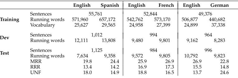
Table 1

XRCE corpus statistics for three different language pairs.

English Spanish English French English German

Training

Sentences 55,761 52,844 49,376

Running words 571,960 657,172 542,762 573,170 506,877 440,682 Vocabulary 25,627 29,565 24,958 27,399 24,899 37,338

Dev Sentences 1,012 994 964

Running words 12,111 13,808 9,480 9,801 9,162 8,283

Test Sentences 1,125 984 996

Running words 7,634 9,358 9,572 9,805 10,792 9,823

MRR 19.8 24.4 25.9 26.9 26.9 22.8

RRR 13.4 14.2 16.9 17.3 15.5 14.8

UNF 18.0 14.9 18.8 16.5 13.7 24.6

experimentation has been made freely available in a new version of toolkit.5 We did not consider the use of the Moses decoder (Koehn et al. 2007) in our experiments because it is not prepared to work in the IMT framework and it does not implement the incremental version of the EM algorithm (it implements the stepwise version, which is unstable in online learning settings, according to Blain, Schwenk, and Senellart [2012]). However, translation quality results reported in Ortiz-Mart´ınez (2011) show that Thot is competitive with Moses for corpora of different complexities.

4.1 Corpora

The experiments were performed using the XRCE, the Europarl, and the EMEA cor-pora. The XRCE corpus (SchlumbergerSema S.A. et al. 2001) consists of translations of XRCE printer manuals from English to three different languages—namely, Spanish, French, and German. Table 1 shows the main figures of the XRCE corpora for training, development, and test partitions. The XRCE corpus is included here because it has been extensively used in the literature to report SMT and IMT results (a complete set of experiments with this corpus is shown in Barrachina et al. [2009]). This feature will allow us to compare the results of our proposed system with those obtained by state-of-the-art systems.

Table 1 also shows three different measures to predict the effectiveness of online learning for this particular translation task, including the modified repetition rate (MRR), the restricted repetition rate (RRR), and the unseenn-gram fraction (UNF) (see Section 3.3). In this work we propose to use only RRR and UNF measures to assess the usefulness of online learning. However, MRR will also be reported so as to give a better idea of the accuracy of these two measures. The three XRCE test sets present moderately high values for the three measures. Slight drops of the RRR measure with respect to the MRR measure are observed (that is, there are repeatedn-grams in the test corpus that were already seen in the training set), suggesting that the repetition rate present in the test sets cannot be fully exploited by online learning.

The Europarl corpus (Koehn 2005) is extracted from the proceedings of the Euro-pean Parliament, which are written in the different languages of the EuroEuro-pean Union.

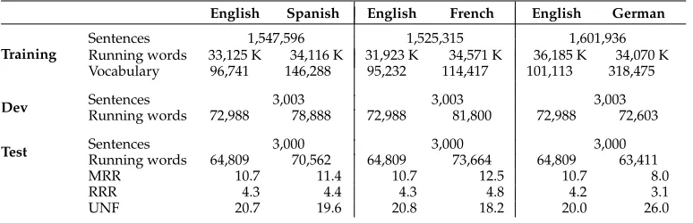
Table 2

Europarl corpus statistics for three different language pairs.

English Spanish English French English German

Training

Sentences 1,547,596 1,525,315 1,601,936

Running words 33,125 K 34,116 K 31,923 K 34,571 K 36,185 K 34,070 K Vocabulary 96,741 146,288 95,232 114,417 101,113 318,475

Dev Sentences 3,003 3,003 3,003

Running words 72,988 78,888 72,988 81,800 72,988 72,603 Test Sentences_{Running words 64,809} 3,000_{70,562 64,809} 3,000_{73,664 64,809} 3,000_63,411

MRR 10.7 11.4 10.7 12.5 10.7 8.0

RRR 4.3 4.4 4.3 4.8 4.2 3.1

UNF 20.7 19.6 20.8 18.2 20.0 26.0

In our experiments we used the version created for the shared task of the ACL 2013 Workshop on Statistical Machine Translation (Bojar et al. 2013). To simplify the experi-ments, all those sentences whose length in words was greater than 40 were removed from the training set. Regarding the language pairs under consideration, again, we will translate from the English language to Spanish, French, and German. Table 2 shows the main figures of training, development, and test sets. The Europarl corpus constitutes one good example of a complex, real-world translation task that is also very well known in the MT scientific community. Regarding the measures to predict the effectiveness of online learning, it should be noted that the MRR measure is much lower than that observed for the XRCE corpora (see Table 1). Moreover, a significant drop in the RRR measure with respect to the MRR is observed, indicating that the vast majority of the repeatedn-grams in the test corpus has already been seen in the training corpus. Therefore, we expect a limited effectiveness of online learning for this task.

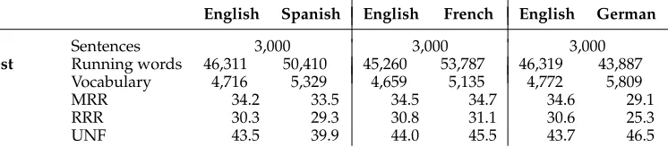
Finally, we also carried out experiments with the EMEA corpus. The EMEA corpus consists of documents from the European Medicines Agency, made available with the OPUS corpora collection (Tiedemann 2009). In this work we extracted specific test sets of 3,000 sentences from the whole set of parallel sentences. Before doing this, we first removed the duplicate sentence pairs contained in this corpus (they represent a very high percentage of the total number of sentence pairs). Table 3 contains some statistics of the resulting corpora. The main interest of the EMEA corpus in our proposed experimentation is that it constitutes an example of an in-domain translation task. The models of the SMT system can be estimated from the out-of-domain Europarl corpus and then used to translate the EMEA corpus, simulating a non-stationary translation task. As it can be seen in Table 3, MRR, RRR, and UNF measures clearly suggest the potential usefulness of online learning in this task (RRR and UNF were calculated using the Europarl training corpus as the out-of-domain corpus).

4.2 Assessment Criteria

Table 3

Statistics for a subset of the EMEA corpus selected for testing purposes. Figures are shown for three different language pairs. RRR and UNF measures have been calculated using the Europarl training set as the out-of-domain corpus.

English Spanish English French English German

Test

Sentences 3,000 3,000 3,000

Running words 46,311 50,410 45,260 53,787 46,319 43,887

Vocabulary 4,716 5,329 4,659 5,135 4,772 5,809

MRR 34.2 33.5 34.5 34.7 34.6 29.1

RRR 30.3 29.3 30.8 31.1 30.6 25.3

UNF 43.5 39.9 44.0 45.5 43.7 46.5

translations with the corresponding target language references of the test set. WER and BLEU measures are intended for its use in the evaluation of the PE scenario:

r

reference translation by computing the minimum number of edit distance operations (substitutions, insertions and deletions) between the hypothesis and the reference translation, divided by the number of reference words.

r

2001) computes the geometric mean of the precision ofn-grams of various lengths between a hypothesis and a set of reference translations multiplied by a factor that penalizes short sentences.

Because we want to evaluate the performance of our proposed SMT system in an IMT scenario, we need to estimate the effort required by the user to produce correct translations using the system. To this end, we use the target references to simulate the translations that the user has in mind. The first translation hypothesis for each given source sentence is compared with a single reference translation and the longest common character prefix (LCCP) is obtained. The first non-matching character is replaced by the corresponding reference character and then a new system translation is produced. This process is iterated until a full match with the reference is obtained. Each computation of the LCCP would correspond to the user looking for the next error and moving the pointer to the corresponding position of the translation hypothesis. We refer to a pointer movement as amouse-action. On the other hand, each character replacement would correspond to akeystroke of the user. If the first non-matching character is the first character of the new system hypothesis in a given interaction, no LCCP computation is needed; that is, no pointer movement would be made by the user. Bearing this in mind, we define the following IMT evaluation measure:

r

is the number of keystrokes plus the number of mouse-actions divided by the total number of reference characters.

In addition to the WER, BLEU, and KSMR measures, in our experimentation we additionally report the learning time in seconds after each training sample presentation. The learning time is important to assess the ability of the learning algorithms to work in a real time scenario. All the experiments were executed on a Windows PC with a 2.00 Ghz Intel Xeon processor with 1GB of memory.

4.3 Experimentation Protocol

We evaluated our techniques by simulating real users. Because the different corpora used in the experiments contained source and target translations, we used the latter to simulate the reference translations that the user has in mind for each source sentence.

This paper studies the application of the online learning paradigm to SMT; therefore the experimentation follows the learning process structured as a sequence of trials that was described in Section 3.1. During this sequence of trials, online learning systems experience some sort of learning curve as they gain knowledge after each training sample presentation. Given that such a learning curve is an important issue when designing online learning algorithms, some of the results reported here include plots with the evolution of cumulative error measures.

It is also interesting to clarify the way in which the different corpora described in Section 4.1 have been used throughout the experimentation. One factor that has influenced the decisions in this regard is the high computational cost of batch retraining. Batch retraining is present in different experiments reported in this work because it provides a valuable reference when assessing the performance of online learning. In such experiments, we have defined specific subsets of the training corpora in order to speed up the experiments. More specifically, the first 10,000 sentences of the XRCE and Europarl corpora have been used.

The decisions regarding the use of the different corpora in the experiments can be summarized as follows. The training sets of the XRCE and Europarl corpora were used to measure the convergence properties of the incremental EM algorithm (Section 4.4). The above-mentioned subset of the training corpora was used to study the impact of the update frequency in the results (Section 4.5), to compare the performance of batch and online learning (Section 4.6), and to analyze the influence of sentence ordering in the system performance (Section 4.7). Finally, in the experiments to test the capability of our online learning techniques to learn from previously estimated models (Section 4.8), we used the training and development sets of the XRCE and Europarl corpora to initialize the system models, and the test sets to obtain translation results. For the system trained with the Europarl corpus, the experimentation is complemented with translation results using the in-domain EMEA corpus.

4.4 EM Algorithm Convergence Experiments

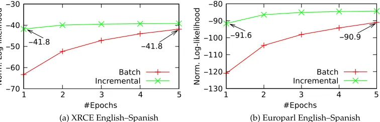
Figure 2

EM convergence experiment comparing the normalized log-likelihood obtained when executing five training epochs of the batch and incremental versions of the EM algorithm. The experiments were executed on the XRCE and Europarl English–Spanish training corpora.

Figure 2 shows the normalized log-likelihood that is obtained when executing up to five training epochs6 _{of the batch and incremental versions of the EM algorithm} (common training schemes in state-of-the-art SMT systems frequently execute five EM training epochs to train the different word-alignment models). Plots were obtained for the XRCE and Europarl training corpora and the three translation directions (from English to Spanish, French, and German). However, in the figure only the XRCE English to Spanish (Figure 2a) and the Europarl English to Spanish (Figure 2b) results are reported7(very similar results were obtained for the other language pairs).

According to the results presented in Figure 2, the incremental EM algorithm is able to obtain a greater normalized log-likelihood than that obtained by the batch EM algorithm for the two corpora under consideration. In addition to this, such a greater log-likelihood can be obtained with fewer EM training epochs. These observed results are due to the fact that the incremental EM algorithm executes complete E and M steps for each training sample, resulting in a much greater rate of model updates per each training epoch (Neal and Hinton 1998).

Note that, according to Equation (24), only one training epoch of the incremental EM algorithm is performed when training HMM-based alignment models (i.e., each training sample is processed only once by the learning algorithm and discarded after-wards). This contrasts with the conventional batch training scheme, in which a few training epochs (typically five) are executed. Hence, to fairly compare batch learning with our proposed online learning strategy, we should observe the relationship between the normalized log-likelihood of the incremental EM algorithm at the first training epoch and that of the fifth training epoch of the batch algorithm. According to the values shown in Figures 2a and 2b, we can appreciate a very small degradation in the log-likelihood (<1% for the Europarl corpus) or no degradation at all.

Because the difference in the log-likelihood between batch and incremental EM algorithms is negligible, we consider that the update rule for HMM-based alignment models given by Equation (24) is able to obtain word-alignment models comparable to those that can be obtained using batch learning. This claim will be supported with additional empirical evidence in Section 4.6.

6 An epoch is a single presentation of all samples in the training set.

Nevertheless, it is possible to take advantage of the better convergence properties of the incremental EM algorithm by slightly modifying the conditions imposed by the online learning framework adopted in this paper (see Section 3.1). In such a framework, only the last sample presented so far to the learning algorithm can be used to modify the model parameters at each trial. This constraint can be slightly relaxed, allowing us to define alternative update rules for the HMM alignment models that execute more than one EM algorithm iteration over each sample. One example of such alternative update rules is described in Appendix A. Empirical results also given in the same appendix show that the obtained log-likelihood and the evaluation measures can be marginally improved with respect to the strict observation of the online learning framework.

Finally, it is worth pointing out that according to the results presented in Figure 2, incremental EM could be suitable to replace batch EM in a batch-learning scenario. However, one disadvantage of applying incremental EM to a batch-learning task is the necessity of storing the sufficient statistics for the whole data set:s1,s2,...,sM. For large data sets, the sufficient statistics may not fit in memory. Nevertheless, this information can be stored on disk and accessed efficiently, because the algorithm reads the data in a sequential manner. By contrast, this disadvantage is totally removed when incremental EM is applied in an online learning scenario, since the sufficient statistics for each training sample are discarded at the end of each trial, or after a finite number of trials for the alternative update rule described in Appendix A.

4.5 Impact of Update Frequency

One important aspect to be clarified when designing PE or IMT systems is the influence of the system update frequency on the obtained performance. It is expected that updat-ing the system in a sentence-wise manner will produce the best results. However, this updating strategy poses efficiency problems because of the necessity of executing model updates in real time. This problem can be alleviated by defining an alternative update strategy in which the training process is delayed until a certain number of samples have been gathered. Delaying model updates may cause performance degradation, but it also constitutes one way to reduce the strong time requirements of a sentence-wise updating strategy. Specifically, if the time between updates is sufficiently high, the use of batch learning techniques could be appropriate (e.g., the training process can be executed overnight), removing the necessity of implementing online learning.

Figure 3

Impact of update frequency when translating the first 10,000 sentences of the English–Spanish language pair of the XRCE and Europarl corpora. A conventional SMT system executed five batch-training epochs every 10, 100, and 1,000 sentences. The system was initialized with empty models and default values for the weights of the log-linear model. Plots show the evolution of the user effort in PE and IMT scenarios measured in terms of cumulative WER and KSMR, respectively.

As it can be observed in Figure 3, the user effort in terms of WER and KSMR was lower when the update frequency was increased. More specifically, batch retraining every 10 samples (Batch10) consistently outperformed the rest of the systems in all cases and retraining every 100 samples (Batch100) was also consistently better than retraining every 1,000 sentences (Batch1000). Sharper curves were obtained when translating the XRCE corpora, probably reflecting that in this corpus, there are groups of sentences with highly different translation difficulties from the system point of view.

Note that, in all cases, the initial WER and KSMR measures are not equal to 100%. This is because of the fact that the system copies to the output all those unknown words contained in the input. In some cases such copied words (names, dates, etc.) are correct words contained in the reference translations.

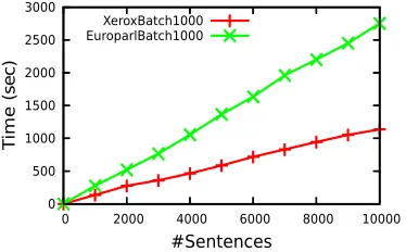
Figure 4

Batch retraining time in seconds as a function of the number of samples presented to the system. Results are shown for the first 10,000 sentences of the XRCE and Europarl training sets. Systems were retrained every 1,000 sentences executing five epochs. Time costs are given in seconds.

10,000 sentences, batch retraining took 19 minutes for the XRCE corpus and 45 minutes for the Europarl corpora. This gives a clear idea of the infeasibility of batch retraining in a sentence-wise updating strategy. Moreover, time costs of batch retraining soon become unaffordable because of their linear growth with the number of translated sentences.

Turning back to the question made at the beginning of this section, experimental results clearly show that it is not possible to obtain the performance of a sentence-wise update strategy if the update frequency is decreased. This constitutes a strong argument in favor of the application of our proposed online learning techniques, which are specifically designed to learn from individual training samples. By contrast, batch learning requires the execution of expensive retraining processes whenever a new sam-ple is presented to the learner. These findings are further supported in the next section, where the performance of batch and online learning systems are compared.

4.6 Batch versus Online Learning, Learning from Scratch

The great impact of frequent updates in the system performance demonstrated in the previous section poses the question of the necessity of replacing conventional batch learning techniques by online learning techniques. EM convergence experiments pro-vided in Section 4.4 showed that the log-likelihood of HMM-based word alignment models using the incremental version of the EM algorithm is competitive with that obtained by using the conventional version. However, it is still unclear if the use of online learning will cause a degradation in the quality of the translations with respect to the use of batch learning.

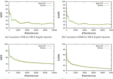
Figure 5 shows the experiments we carried out to demonstrate the effectiveness of online learning. For this purpose, we compared the performance of a batch system executing five training epochs every 10 sentences (Batch10) with that of an online system (Online). Plots show the evolution of the user effort required to obtain correct translations. This effort is measured in terms of cumulative WER and KSMR for the PE and IMT scenarios, respectively. Initial models were empty in all cases. We report the results obtained when translating the first 10,000 sentences of the English–Spanish XRCE (Figures 5a and 5b) and Europarl training corpora (Figures 5c and 5d). Very similar results were obtained for English–French and English–German language pairs.

Figure 5

Comparison between batch and online learning when translating the first 10,000 sentences of the English–Spanish language pair of the XRCE and Europarl corpora. The batch learning system executed five training epochs every 10 sentences. The system was initialized with empty models and default values for the log-linear weights. Plots show the evolution of the user effort in the PE and IMT scenarios measured in terms of cumulative WER and KSMR, respectively.

higher update frequency of online learning, since the SMT models are extended for each individual training pair. It should be noted that the shape of the curves obtained with online learning is very similar to that of batch learning. This implies that incremental EM presents a stable behavior, which contrasts with the instability of the stepwise EM algorithm reported in Blain, Schwenk, and Senellart (2012). Finally, it is also worthy of note that the results also show that the system is able to learn from scratch.

It is also illustrative to carry out a descriptive analysis of the learning times per training sample that were obtained during this experiment. Figure 6 shows a boxplot summarizing the main statistics of the learning times for the XRCE and Europarl corpora. As it can be seen, the boxplot clearly show the small time cost of the learning process for the two different corpora under consideration. Specifically, the learning time was never greater than 1 second, and the median times were 0.03 and 0.16 seconds for the XRCE and the Europarl corpora, respectively. The learning time was greater for the Europarl corpus because of the greater length in words of the sentence pairs with respect to that of the XRCE corpus.

4.7 Ordering Effects

Figure 6

Boxplots of the time cost per each individual training sample required to train the first 10,000 sentences of the XRCE and Europarl training corpora using our proposed online learning techniques. Times are measured in seconds.

its parameters are modified to minimize cumulative prediction error. Hopefully, this modification will allow the system to provide more accurate predictions for similar samples. However, modifying parameters may also produce lateral effects. A lateral effect can cause the system to generate a wrong prediction for a given sample because of undesired changes in the learning algorithm parameters. One possible way to minimize the number of lateral effects is by processing similar samples in consecutive trials.

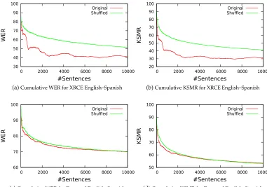
Figure 7 shows the experiments we executed to test the influence of corpus or-dering in both WER and KSMR results when translating the first 10,000 sentences of the English–Spanish XRCE and Europarl training corpora by means of an online SMT system. For both tasks we translated the original portion of the training corpus and the same portion after being randomly shuffled.

As it can be seen in Figure 7, the obtained results were generally better for the original corpora than for the shuffled ones. The reason for the improved results is due to the fact that, in the original corpora, similar sentences appear more or less contiguously (because of the organization of the contents of the printer manuals for the XRCE corpus or to the chronological order of the parliamentary sessions for the Europarl corpus). This circumstance increases the accuracy of online learning, since with the original corpora the number of lateral effects occurred between the translation of similar sentences is decreased. By contrast, the accuracy was worse for shuffled corpora. Shuffling causes similar sentences to no longer appear contiguously and thus, the number of lateral effects that may occur between the translation of similar sentences is increased.

The differences between the results of original and shuffled corpora were much greater for the XRCE corpus than for the Europarl corpus. One possible explanation for this phenomenon is the lower repetition rate of the latter corpus. For low repetition rates, the number of lateral effects between the translation of similar sentences will be lower, since such sentences appear in a small number.

4.8 Learning from Previously Estimated Models

Figure 7

Impact of sentence ordering when translating the first 10,000 sentences of the English–Spanish language pair of the XRCE and Europarl corpora. Such sentences were presented in their original order or randomly shuffled. The system was initialized with empty models and default values for the weights of the log-linear model. The different plots show the evolution of the user effort in the PE and IMT scenarios measured in terms of cumulative WER and KSMR, respectively.

SMT system is a system that is not able to take advantage of user feedback after each translation, whereas the online SMT system uses the new sentence pairs provided by the user to revise the statistical models. Both systems used log-linear models trained in batch mode by means of the XRCE or the Europarl training corpora (five training epochs were executed). The weights of the log-linear model were adjusted for the corresponding development corpora via MERT.

Table 4

BLEU, WER, and KSMR results for the XRCE test corpora using conventional (batch learning without retraining) and online SMT systems. Both systems used MERT to adjust log-linear weights. The average online learning time (LT) in seconds is shown for the online system.

Corpus SMT system BLEU WER KSMR LT (sec)

Eng–Spa conventional_online 58.3_64.0±_±2.4_{2.4 28.1}32.5_±±_1.71.9 _16.619.3_±±_1.11.2 _0.06

-Eng–Fre conventional 32.2±2.2 63.7±2.2 36.7±1.2 -online 43.7±2.3 48.4±2.2 30.3±1.2 0.09

Eng–Ger conventional 20.5±1.9 72.4±1.9 42.9±1.1 -online 28.9±2.1 61.7±2.1 37.0±1.3 0.07

to obtain refined predictions of the impact of online learning in the results. The average learning times allow the system to be used in a real-time scenario.

Additionally, in Table 5 we show a comparison of the KSMR results obtained by our proposed online SMT system, with those obtained by different state-of-the-art IMT systems described in the literature. These IMT systems are based on different trans-lation approaches, including the alignment templates (AT), the stochastic finite-state transducer (SFST), and the phrase-based (PB) approaches to IMT (see Barrachina et al. [2009] for more details). AT and SFST systems follow the word graph-based approach to generate the IMT suffixes, whereas the PB system retranslates the source sentence at each interaction of the IMT process. Experiments reported in Barrachina et al. (2009) showed that word graph–based systems are much faster than systems that retranslate the source sentence at each interaction, but obtain slightly worse results. Because quick response times are critical in an IMT scenario, the majority of the IMT systems reported in the literature, as well as the one proposed here, follow a word graph–based imple-mentation strategy. Our system significantly outperformed the results obtained by the state-of-the-art systems, except those of the PB system for English to Spanish. Even in this case, our system obtained slightly better results.

4.8.2 Europarl Experiments.Table 6 shows the translation results from English to Spanish, French, and German for the Europarl corpus when using conventional and online SMT systems. Again, BLEU, WER, and KSMR measures for conventional and online SMT

Table 5

KSMR results of the comparison of our system with online learning and three different

state-of-the-art IMT conventional systems. The experiments were executed on the XRCE corpora. Best results are shown in bold.

Corpus AT PB SFST Online