GRAph Parallel Actor Language — A
Programming Language for Parallel
Graph Algorithms
Thesis by
Michael deLorimier
In Partial Fulfillment of the Requirements
for the Degree of
Doctor of Philosophy
California Institute of Technology
Pasadena, California
2013
c
2013
Michael deLorimier
Abstract
We introduce a domain-specific language, GRAph PArallel Actor Language, that enables
parallel graph algorithms to be written in a natural, high-level form. GRAPAL is based on
our GraphStep compute model, which enables a wide range of parallel graph algorithms
that are high-level, deterministic, free from race conditions, and free from deadlock.
Pro-grams written in GRAPAL are easy for a compiler and runtime to map to efficient parallel
field programmable gate array (FPGA) implementations. We show that the GRAPAL
com-piler can verify that the structure of operations conforms to the GraphStep model. We
allocate many small processing elements in each FPGA that take advantage of the high
on-chip memory bandwidth (5x the sequential processor) and process one graph edge per clock cycle per processing element. We show how to automatically choose parameters for
the logic architecture so the high-level GRAPAL programming model is independent of the
target FPGA architecture. We compare our GRAPAL applications mapped to a platform
with four 65 nm Virtex-5 SX95T FPGAs to sequential programs run on a single 65 nm
Xeon 5160. Our implementation achieves a total mean speedup of 8x with a maximum speedup of 28x. The speedup per chip is 2x with a maximum of 7x. The ratio of energy used by our GRAPAL implementation over the sequential implementation has a mean of
Contents
Abstract iii
1 Introduction 1
1.1 High-Level Parallel Language for Graph Algorithms . . . 2
1.2 Efficient Parallel Implementation . . . 4
1.3 Requirements for Efficient Parallel Hardware for Graph Algorithms . . . . 8
1.3.1 Data-Transfer Bandwidths . . . 8
1.3.2 Efficient Message Handling . . . 10
1.3.3 Use of Specialized FPGA Logic . . . 10
1.4 Challenges in Targeting FPGAs . . . 11
1.5 Contributions . . . 12
1.6 Chapters . . . 14
2 Description and Structure of Parallel Graph Algorithms 16 2.1 Demonstration of Simple Algorithms . . . 16
2.1.1 Reachability . . . 16
2.1.2 Asynchronous Bellman-Ford . . . 17
2.1.3 Iterative Bellman-Ford . . . 19
2.2 GraphStep Model . . . 21
2.3 Graph Algorithm Examples . . . 23
2.3.1 Graph Relaxation Algorithms . . . 23
2.3.2 Iterative Numerical Methods . . . 25
2.3.3 CAD Algorithms . . . 26
2.3.5 Web Algorithms . . . 27
2.4 Compute Models and Programming Models . . . 27
2.4.1 Actors . . . 28
2.4.2 Streaming Dataflow . . . 28
2.4.3 Bulk-Synchronous Parallel . . . 30
2.4.4 Message Passing Interface . . . 31
2.4.5 Data Parallel . . . 31
2.4.6 GPGPU Programming Models . . . 32
2.4.7 MapReduce . . . 33
2.4.8 Programming Models for Parallel Graph Algorithms . . . 34
2.4.9 High-Level Synthesis for FPGAs . . . 36
3 GRAPAL Definition and Programming Model 38 3.1 GRAPAL Kernel Language . . . 38
3.2 Sequential Controller Program . . . 44
3.3 Structural Constraints . . . 45
4 Applications in GRAPAL 48 4.1 Bellman-Ford . . . 48
4.2 ConceptNet . . . 50
4.3 Spatial Router . . . 53
4.4 Push-Relabel . . . 57
4.5 Performance . . . 59
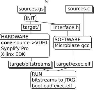
5 Implementation 62 5.1 Compiler . . . 62
5.1.1 Entire Compilation and Runtime Flow . . . 64
5.1.1.1 Translation from Source to VHDL . . . 67
5.1.1.2 Structure Checking . . . 70
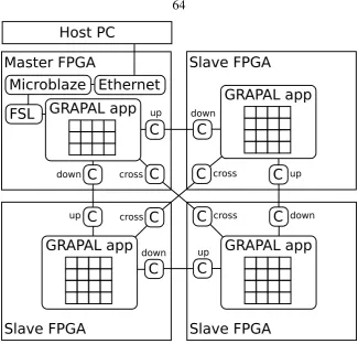
5.2 Logic Architecture . . . 71
5.2.1.1 Support for Node Decomposition . . . 82
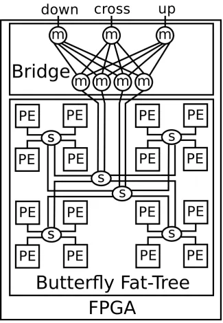
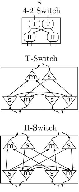
5.2.2 Interconnect . . . 85
5.2.2.1 Butterfly Fat-Tree . . . 88
6 Performance Model 90 6.1 Model Definition . . . 91
6.1.1 Global Latency . . . 92
6.1.2 Node Iteration . . . 95
6.1.3 Operation Firing and Message Passing . . . 95
6.2 Accuracy of Performance Model . . . 97
7 Optimizations 99 7.1 Critical Path Latency Minimization . . . 100
7.1.1 Global Broadcast and Reduce Optimization . . . 100
7.1.2 Node Iteration Optimization . . . 102
7.2 Node Decomposition . . . 102
7.2.1 Choosing∆limit . . . 104
7.3 Message Synchronization . . . 106
7.4 Placement for Locality . . . 108
8 Design Parameter Chooser 115 8.1 Resource Use Measurement . . . 116
8.2 Logic Parameters . . . 117
8.3 Memory Parameters . . . 121
8.4 Composition to Full Designs . . . 123
9 Conclusion 125 9.1 Lessons . . . 125
9.1.1 Importance of Runtime Optimizations . . . 125
9.1.2 Complex Algorithms in GRAPAL . . . 125
9.2 Future Work . . . 126
9.2.1 Extensions to GRAPAL . . . 126
9.2.2 Improvement of Applications . . . 127
9.2.3 Logic Sharing Between Methods . . . 127
9.2.4 Improvements to the Logic Architecture . . . 128
9.2.5 Targeting Other Parallel Platforms . . . 128
Bibliography 129
A GRAPAL Context-Free Grammar 139
B Push-Relabel in GRAPAL 141
Chapter 1
Introduction
My Thesis:GRAPAL is a DSL for parallel graph algorithms that enables them to be written
in a natural, high-level form. Computations restricted to GRAPAL’s domain are easy to
map to efficient parallel implementations with large speedups over sequential alternatives.
Parallel execution is necessary to efficiently utilize modern chips with billions of
tran-sistors. There exists a need for programming models that enable high-level, correct and
ef-ficient parallel programs. To describe a parallel program on a low level, concurrent events
must be carefully coordinated to avoid concurrency bugs, such as race conditions, deadlock
and livelock. Further, to realize the potential for high performance, the program must
dis-tribute and schedule operations and data across processors. A good parallel programming
model helps the programmer capture algorithms in a natural way, avoids concurrency bugs,
enables reasonably efficient compilation and execution, and abstracts above a particular
machine or architecture. Three desirable qualities of a programming model are that it is
general and captures a wide range of computations, high level so concurrency bugs are rare
or impossible, and easy to map to an efficient implementation. However, there is a tradeoff
between a programming model being general, high-level and efficient.
The GRAPAL programming language is specialized to parallel graph algorithms so it
can capture them on a high level and translate and optimize them to an efficient low-level
form. This domain-specific language (DSL) approach, which GRAPAL takes, is a common
approach used to improve programmability and/or performance by trading off generality.
GRAPAL is based on the GraphStep compute model [1, 2], in which operations are
the computation match the structure of the graph. GRAPAL enables programs to be
de-terministic without race conditions or deadlock or livelock. Each run of a dede-terministic
program gets the same result as other runs and is independent of platform details such as
the number of processors. The structure of the computation is constrained by the
Graph-Step model, which allows the compiler and runtime to make specialized scheduling and
implementation decisions to produce an efficient parallel implementation. For algorithms
in GraphStep, memory bandwidth is critical, as well as network bandwidth and network
latency. The GRAPAL compiler targets FPGAs, which have high on-chip memory
band-width (Table 1.1) and allow logic to be customized to deliver high network bandband-width with
low latency. In order to target FPGAs efficiently, the compiler needs the knowledge of the
structure of the computation that is provided by restriction to the GraphStep model.
Graph-Step tells the compiler that operations are local to nodes and edges and communicate by
sending messages along the graph structure, that the graph is static, and that parallel activity
is sequenced into iterations. The domain that GRAPAL supports, as a DSL, is constrained
on top of GraphStep to target FPGAs efficiently. Local operations are feed-forward to make
FPGA logic simple and high-throughput. These simple primitive operations are composed
by GraphStep into more complex looping operations suitable for graph algorithms.
We refer to the static directed multigraph used by a GraphStep algorithm asG= (V, E).
V is the set of nodes andE is the set of edges.(u, v)denotes a directed edge fromutov.
1.1
High-Level Parallel Language for Graph Algorithms
An execution of a parallel program is a set of events whose timing is a complex function of
machine details which include operator latencies, communication latencies, memory and
cache sizes, and throughput capacities. These timing details affect the ordering of
low-level events, making it difficult or impossible to predict the relative ordering of events.
When operations share state, the order of operations can affect the outcome due to write
after read, read after write, or write after write dependencies. When working at a low
level, the programmer must ensure the program is correct for any possible event ordering.
exposed late, when an unlikely ordering occurs or when the program is run with a different
number of processors. Even if all nondeterministic outcomes are correct, it is difficult
to understand program behavior due to lack of repeatability. nondeterminism can raise a
barrier to portability since the machine deployed and the test machine often expose different
orderings.
Deadlock occurs when there is a cycle of N processes in which each process, Pi, is
holding resource,Ri, and is waiting forP(i+1) modN to releaseR(i+1) modN before releasing
Ri. When programming on a primitive level, with locks to coordinate sharing of resources,
deadlock is a common concurrency bug. Good high-level models prevent deadlock or help
the programmer avoid deadlock. Many data-parallel models restrict the set of possible
concurrency patterns by excluding locks from the model, thereby excluding the possibility
of deadlock. In transactional memory the runtime (with possible hardware support) detects
deadlock then corrects it by rolling back and re-executing.
Even if it seems that deadlock is impossible from a high-level perspective, bufferlock,
a type of deadlock, can occur in message passing programs due to low-level resource
con-straints. Bufferlock occurs when there is a cycle of hardware buffers where each buffer is
full and is waiting for empty slots in the next buffer [3]. Since bufferlock depends on
hard-ware resource availability, this is another factor that can limit portability across machines
with varying memory or buffer sizes. For example, it may not work to execute a program
on a machine with more total memory but less memory per processor than the machine it
was tested on.
The GraphStep compute model is designed to capture parallel graph algorithms at a
high level where they are deterministic, outcomes do not depend on event ordering, and
deadlock is impossible. A GraphStep program works on a static directed multigraph in
which state-holding nodes are connected with state-holding edges. First, GraphStep
syn-chronizes parallel operations into iterations, so no two operations that read or write to
the same state can occur in the same iteration. Casting parallel graph algorithms as
iter-ative makes them simple to describe. In each iteration, or graph-step, active nodes start
by performing an update operation that accesses local state only and sends messages on
operation that accesses local edge state only and sends a single message to the edge’s
destination node. Destination nodes then accumulate incoming messages with a reduce
operation and store the result for the update operation in the next graph-step. A global
barrier-synchronization separates thesereduceoperations at the end of one graph-step from
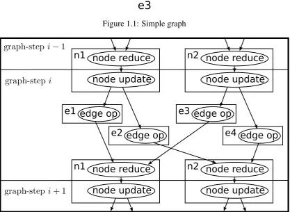
theupdateoperations at the beginning of the next. Figure 1.2 shows the structure of these
operations in a graph-step for the simple graph in Figure 1.1. Since node update and edge
operations act on local state only and fire at most once per node per graph-step, there is
no possibility for race conditions. With the assumption that the reduce operation is
com-mutative and associative, the outcome of each graph-step is deterministic. All operations
are atomic so the programmer does not have to reason about what happens in each
opera-tion, or whether to make a particular operation atomic. There are no dependency cycles, so
deadlock on a high level is impossible. Since there is one message into and one message
out of each edge, the compiler can calculate the required message buffer space, making
bufferlock impossible.
1.2
Efficient Parallel Implementation
Achieving high resource utilization is usually more difficult when targeting parallel
ma-chines than when targeting sequential mama-chines. If the programmer is targeting a range
of parallel machine sizes, then program efficiency must be considered for each possible
number of parallel processors. In a simple abstract sequential model, performance is only
affected by total computation work. That is, if T is the time to complete a computation
andW is the total work of the computation, then T = W. In general, parallel machines vary over more parameters than sequential machines. One of the simplest parallel abstract
machine models is Parallel Random Access Machine (PRAM) [4], in which the only
pa-rameter that varies is processor count, P. In the PRAM model, runtime depends is the
maximum amount of time used by any processor: T = maxP
i=1wi. Minimizing work, W = PP
i=1wi, still helps minimize T, but extra effort must be put into load balancing
Figure 1.1: Simple graph
Figure 1.2: The computation structure of a graph-step on the graph in Figure 1.1 is shown here. In graph-stepi, node update operations at nodes n1 and n2 send to edge operations at edges e1, e2, e3 and e4, which send to node reduce operations at nodes n1 and n2.
most relevant to GraphStep is the bulk-synchronous parallel model (BSP), [5] which has
processor count, a single parameter to model network bandwidth, and a single parameter
to model network latency. To optimize for BSP, computation is divided into supersteps,
and time spent in a superstep, S, needs to be minimized. The time spent in a superstep
performing local operations isw = maxP
i=1wi, wherewi is the time spent by processori.
The time spent communicating between processors ishg, where his the number of
mes-sages andg is the scaling factor for network load. The inverse of network bandwidth is the
primary contributor tog. Each superstep ends with a global barrier synchronization whose
synchronization time:
S =w+hg+l
Now work in each superstep (PP
i=1wi) needs to be minimized and load balanced, and
[image:13.595.147.286.174.429.2]network traffic needs to be minimized.
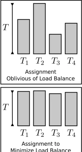
Figure 1.3: Work should be load bal-anced across the 4 processors to min-imize runtime (T = maxP
i=1Ti in the
PRAM model).
Figure 1.4: This linear topology of nodes or operators should be assigned to the 2 processors to minimize network traffic so
h in the BSP model is 1(bottom) not 7
(top).
An efficient execution of a parallel program requires a good assignment of operations to
processors and data to memories. To minimize time spent according to the PRAM model,
operations should be load-balanced across processors (Figure 1.3). In BSP, message
pass-ing between operations can be the bottleneck due to too little network bandwidth, g. To
minimize message traffic, a local assignment should be performed so operations that
com-municate are assigned to the same processor (Figure 1.4). This assignment for locality
should not sacrifice the load-balance, so bothwandhgare minimized. Most modern
paral-lel machines have non-uniform memory access (NUMA) [6] in which the distance between
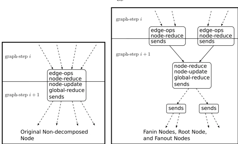
[image:13.595.363.495.199.418.2]mem-Figure 1.5: Decomposition transforms a node into smaller pieces that require less memory and less compute per piece. The commutativity and associativity of reduce operators allows them to be decomposed into fanin nodes. Fanout nodes simply copy messages.
ory which it can access with relatively low latency and high bandwidth compared to other
processors’ memories. In BSP each processor has its own memory and requires message
passing communication for operations at one processor to access state stored at others. For
graph algorithms to use BSP machines efficiently operations on nodes and edges should
be located on the same processor as the node and edge objects. For graph algorithms to
minimize messages between operations, neighboring nodes and edges should be located
on the same processor whenever possible. Finally, load-balancing nodes and edges across
processors helps load-balance operations on nodes and edges. In general, this assignment
of operations and data to processors and memories may be done by part of the program,
requiring manual effort by the programmer, by the compiler, or by the runtime or OS. For a
good assignment either the programmer customizes the assignment for the program, or the
programming model exposes the structure of the computation and graph to the compiler
and runtime.
GraphStep abstracts out machine properties and assignment of operation and data to
processors. The GRAPAL compiler and runtime has knowledge of the parameters of the
machine being targeted so it can customize the computation to the machine. The GRAPAL
runtime uses the knowledge of the structure of the graph to assign operations and data to
processors and memories so machine resources can be utilized efficiently. The runtime
tries to assign neighboring nodes and edges to processors so that communication work,hg,
is minimized. Edge objects are placed with their successor nodes so an edge operation
may get an inter-processor message on its input but never needs to send an inter-processor
inter-processor message, so the runtime minimizes inter-inter-processor edges. For GraphStep
algo-rithms, the runtime knows that the time spent on an active nodevwith indegree∆−(v)and outdegree ∆+(v)is proportional tomax(∆−(v),∆+(v)). Therefore, computation time in
a BSP superstep at processori, wherev(i)is the set of active nodes, is:
wi =
X
v∈v(i)
max(∆−(v),∆+(v))
Load balancing is minimizingmaxPi=1wiso nodes are assigned to processors to balance the
number of edges across processor. For many graphs, a few nodes are too large to be load
balanced across many processors (|E|/P < maxv∈V max(∆−(v),∆+(v))). The runtime
must break nodes with large indegree and outdegree into small pieces so the pieces can be
load balanced (Figure 1.5). Node decomposition decreases the outdegree by allocating
in-termediate fanout nodes between the original node and its successor edges, and fanin nodes
between the original node and predecessor edges. Fanout nodes simply copy messages and
fanin nodes utilize the commutativity and associativity of reduce operations to break the
reduce into pieces. Finally, restriction to a static graph simplifies assignment since it only
needs to be performed once, when the graph is loaded.
1.3
Requirements for Efficient Parallel Hardware for
Graph Algorithms
This section describes machine properties that are required for efficient execution of
Graph-Step algorithms.
1.3.1
Data-Transfer Bandwidths
Data-transfer bandwidths are a critical factor for high performance. In each iteration, or
graph-step, the state of each active node and edge must be loaded from memory, making
memory bandwidth critical. Each active edge which connects two nodes that are assigned
XC5VSX95T 3 GHz Xeon 5160 3 GHz Xeon 5160
FPGA One Core Both Cores
On-chip Memory Bandwidth 4000 Gbit/s 380 Gbit/s 770 Gbit/s
On-chip Communication Bandwidth 7000 Gbit/s N/A 770 Gbit/s
Table 1.1: Comparison of FPGA and Processor on-chip memory bandwidth and on-chip raw communication bandwidth. Both chips are of the same technology generation, with a feature size of 65 nm. The FPGA frequency is 450 MHz, which is the maximum supported by BlockRAMs in a Virtex-5 with speed grade -1 [7]. The processor bandwidth is the maximum available from the L1 cache [8]. All devices can read and write data concurrently at the quoted bandwidths. Communication bandwidth for the FPGA is the bandwidth of wires that cross two halves of the reconfigurable fabric [9, 10]. Communication bandwidth for the dual-core Xeon is the bandwidth between the two cores. Since cores communicate through caches, this bandwidth is the same as on-chip memory bandwidth.
critical (g in the BSP model). For high performance, GraphStep algorithms should be
implemented on machines with high memory and network bandwidth. Table 1.1 shows
on-chip memory and on-chip communication bandwidths for an Intel Xeon 5160 dual core
and for a Virtex-5 FPGA. Both chips are of the same technology generation, with a feature
size of 65 nm. Since the raw on-chip memory and network bandwidths of the FPGA are
[image:16.595.335.527.435.548.2]5times and9times higher, respectively, than the Xeon, our GRAPAL compiler should be able to exploit FPGAs to achieve high performance.
Figure 1.6: A regular mesh with nearest neighbor communication is partitioned into squares with 4 nodes per partition. Each of the 4 partitions shown here is identified with a processor.
1.3.2
Efficient Message Handling
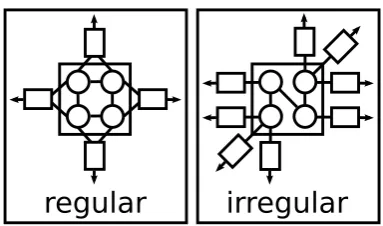
Graph applications typically work on sparse, irregular graphs. These include semantic
net-works, the web, finite element analysis, circuit graphs, and social networks. A sparse graph
has many fewer edges than a fully connected graph, and an irregular graph has no regular
structure of connections between nodes. To efficiently support graphs with an irregular
structure the machine should perform fine-grained message passing efficiently. For regular
communication structures, small values can be packed into large coarse-grained messages.
An example of a regular high-level structure is a 2-dimensional mesh with nodes that
com-municate with their four nearest neighbors. This mesh can be partitioned into rectangles
so nodes in one partition only communicate with nodes in the four neighboring partitions
(Figure 1.6). High-level messages between nodes are then packed into low-level,
coarse-grained messages between neighboring partitions (Figure 1.7). When an irregular
struc-ture is partitioned, each partition is connected to many others so each connection does not
have enough values to pack into a large coarse-grained message. High-level messages in
GraphStep applications usually contain one scalar or a few scalars, so the target machine
needs to handle fine-grained messages efficiently. Conventional parallel clusters typically
only handle coarse-grained communication with high throughput. MPI implementations
get two orders of magnitude less throughput for messages of a few bytes than for kilobyte
messages [11]. Grouping fine-grained messages into coarse-grained messages has to be
described on a low level and cannot be done efficiently in many cases. FPGA logic can
process messages with no synchronization overhead by streaming messages into and out of
a pipeline of node and edge operators. Section 5.2.1 explains how these pipelines handle a
throughput of one fine-grained message per clock cycle.
1.3.3
Use of Specialized FPGA Logic
The structure of the computation in each graph-step is known by the compiler: Node update
operators send to edges, edges operations fire and send to node reduce operators, then node
reduce operators accumulate messages (Figure 1.2). By targeting FPGAs, the GRAPAL
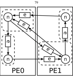
Compo-nents of FPGA logic are often organized as spatial pipelines which stream data through
registers and logic gates. We implement GraphStep operators as pipelines so each operator
has a throughput of one operation per cycle. We group an edge operator, a node reduce
operator, a node update operator, and a global reduce operator into each PE. This means
that the only inter-PE messages are sent from a node update operation to an edge
opera-tion, which results in lower network traffic (hin BSP) than the case where each operator
can send a message over the network. Since memory bandwidth is frequently a bottleneck,
we allocate node and edge memories for the operators so they do not need to compete for
shared state. Section 5.2.1 explains how PEs are specialized so each active edge located at
a PE uses only one of the PE pipeline’s slots in a graph-step. In terms of active edges per
cycle, specialized PE logic gives a speedup of30times over a sequential processor that is-sues one instruction per cycle: Sequential code for a PE executes30instructions per active edge (Figure 5.8). Further, by using statically managed on-chip memory there are no stalls
due to cache misses.
Like BSP, GraphStep performs a global barrier synchronization at the end of each
graph-step. This synchronization detects when message and operation activity has
qui-esced, and allows the next graph-step after quiescence. We specialize the FPGA logic to
minimize the time of the global barrier synchronization,l. By dedicating special logic to
detect quiescence and by dedicating low-latency broadcast and reduce networks for the
global synchronization signals we reducelby55%.
1.4
Challenges in Targeting FPGAs
High raw memory and network bandwidths and customizable logic give FPGAs a
perfor-mance advantage. In order to use FPGAs, the wide gap between the high-level GraphStep
programs and low-level FPGA logic must be bridged. In addition to capturing parallel
graph algorithms on a high-level, GRAPAL constrains program to a domain of
computa-tions that are easy to compile to FPGA logic. Local operacomputa-tions on nodes and edges are
feed forward so they don’t have loops or recursion. This makes it simple to compile
cycle. The graph is static so PE logic is not made complex by the need for allocation,
deletion, and garbage collection functionality. GRAPAL’s restriction that there is at most
one operation per edge per graph-step allows the implementation to use the FPGA’s small,
distributed memories to perform message buffering without the possibility of bufferlock or
cache misses.
Each FPGA model has a unique number of logic and memory resources, and a compiled
FPGA program (bitstream) specifies how to use each logic and memory component. The
logic architecture output by the GRAPAL compiler has components, such as PEs, whose
resource usage is a function of the input application. To keep the programming model
ab-stract above the target FPGA, the GRAPAL compiler customizes the output architecture to
the amount of resources on the target FPGA platform. Unlike typical FPGA programming
languages (e.g. Verilog), where the program is customized by the programmer for the target
FPGA’s resource count, GRAPAL supports automated scaling to large FPGAs. Chapter 8
describes how the compiler chooses values for logic architecture parameters for efficient
use of FPGA resources.
1.5
Contributions
• GraphStep compute model: We introduce GraphStep as a minimal compute model
that supports a wide range of high-level parallel graph algorithms with highly efficient
implementations. We chose to make the model iterative so it is easy to reason about
tim-ing behavior. We chose to base communication on message passtim-ing to make execution
efficient and so the programmer does not have to reason about shared state. GraphStep
is interesting to us because we think it is the simplest model that is based on iteration
and message passing and captures a wide range of parallel graph algorithms. Chapter 2
explains why GraphStep is a useful compute model, particularly how it is motivated by
parallel graph algorithms and how it is different from other parallel models. This work
explores the ramifications of using GraphStep: how easy it is to program, what kind of
• GRAPAL programming language:
We create a DSL that exposes GraphStep’s graph concepts and operator concepts to the
programmer. We identify constraints on GraphStep necessary for a mapping to simple,
efficient, spatial FPGA logic, and include them in GRAPAL. We show how to statically
check that a GRAPAL program conforms to GraphStep so that it has GraphSteps’s safety
properties.
• Demonstration of graph applications in GRAPAL: We demonstrate that GRAPAL
can describe four important parallel graph algorithm benchmarks: Bellman-Ford to
com-pute single-source shortest paths, the spreading activation query for the ConceptNet
se-mantic network, a parallel graph algorithm for the netlist routing CAD problem, and the
Push-Relabel method for single-source, single-sink Max Flow/Min Cut.
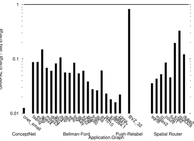
• Performance benefits for graph algorithms in GRAPAL:We compare our benchmark
applications written in GRAPAL and executed on a platform of4FPGAs to sequential versions executed on a sequential processor. We show a mean speedup of8times with a maximum speedup of28times over the sequential programs. We show a mean speedup per chip of2times with a maximum speedup of7times. We also show the energy cost of GRAPAL applications compared to sequential versions has a mean ratio of1/10with a minimum of1/80.
• Compiler for GRAPAL:We show how to compile GRAPAL programs to FPGA logic.
Much of the compiler uses standard compilation techniques to get from the source
pro-gram to FPGA logic. We develop algorithms specific to GRAPAL to check that the
structure of the program conforms to GraphStep. These checks prevent race conditions
and enable the use of small-distributed memories without bufferlock.
• Customized logic architecture: We introduce a high-performance, highly customized
FPGA logic architecture for GRAPAL. This logic architecture is output by the compiler
and is specialized to GraphStep computations in general, and also the compiled
GRA-PAL program in particular. We show how to pack many processing elements (PEs) into
an FPGA with a packet-switched network. We show how to architect PE logic to input
messages, perform node and edge operations, and output messages at a high throughput,
fine-grained messages with no overhead. We show how to use small, distributed memories at
high throughput.
• Evaluation of optimizations: We demonstrate optimizations for GRAPAL that are
en-abled by restrictions to its domain. We show a mean reduction of global barrier
synchro-nization latency of55% by dedicating networks to global broadcast and global reduce. We show a mean speedup of1.3due to decreasing network traffic by placing for locality. We show a mean speedup of2.6due to improving load balance by performing node de-composition. We tune the node decomposition transform and show that a good target size
for decomposed nodes is the maximum size that fits in a PE. We evaluate three schemes
for message synchronization that trade off between global barrier synchronization costs
(l) on one hand and computation and communication throughput costs (w+hg) on the other. We show that the best synchronization scheme delivers a mean speedup of4over a scheme that does not use barrier synchronization. We show that the best synchronization
scheme delivers a mean speedup of1.7over one that has extra barrier synchronizations used to decreasew+hg.
• Automatic choice of logic parameters: We show how the compiler can automatically
choose parameters to specialize the logic architecture of each GRAPAL program to the
target FPGA. With GRAPAL, we provide an example of a language that is abstract above
a particular FPGA device while being able to target a range of devices. We show that
our compiler can achieve a high utilization of the device, with95%to97%of the logic resources utilized and 89% to 94% of small BlockRAM memories utilized. We show that the mean performance achieved for the choices made by our compiler is within1%
of the optimal choice.
1.6
Chapters
The rest of this thesis is organized as follows: Chapter 2 gives an overview of parallel graph
algorithms, shows how they are captured by the GraphStep compute model, and compares
GraphStep to other parallel compute and programming models. Chapter 3 explains the
Chap-ter 4 presents the example applications in GRAPAL, and evaluates their performance when
compiled to FPGAs compared to the performance for sequential versions. Chapter 5
ex-plains the GRAPAL compiler and the logic architecture generated by the compiler.
Chap-ter 6 gives our performance model for GraphStep, which is used to evaluate bottlenecks in
GRAPAL applications and evaluate the benefit of various optimizations. Chapter 7
evalu-ates optimizations that improve the assignment of operations and data to PEs, optimizations
that decrease critical path latency, and optimizations that decrease the cost of
synchroniza-tion. Chapter 8 explains how the compiler chooses values for parameters of its output logic
architecture as a function of the GRAPAL application and of FPGA resources. Finally
Chapter 2
Description and Structure of Parallel
Graph Algorithms
This chapter starts by describing simple representative examples of parallel graph
algo-rithms. We use the Bellman-Ford single-source shortest paths algorithm [12] to motivate
the iterative nature of the GraphStep compute model. GraphStep is then described in detail.
An overview is given of domains of applications that work on parallel graph algorithms.
The GraphStep compute model is compared to related parallel compute models and
perfor-mance models.
2.1
Demonstration of Simple Algorithms
First we describe simple versions of Reachability and Bellman-Ford in which parallel
ac-tions are asynchronous. Next, the iterative nature of GraphStep is motivated by
show-ing that the iterative form Bellman-Ford has exponentially better time-complexity than the
asynchronous form.
2.1.1
Reachability
Source to sink reachability is one of the simplest problems that can be solved with parallel
graph algorithms. A reachability algorithm inputs a directed graph and a source node then
labels each node for which there exists a path from the source to the node. Figure 2.1
class node
boolean reachable set<node> neighbors setReachable()
if not reachable reachable := true
for each n in neighbors n.setReachable()
setAllReachable(node source) for each node n
n.reachable := false source.setReachable()
Figure 2.1: Reachability pseudocode
activity by calling the setReachablemethod at the source node. When invoked on a
node not yet labeled reachable,setReachablepropagates itself to each successor node.
If the node is labeled reachable thensetReachable doesn’t need to do anything. This
algorithm can be interpreted as a sequential algorithm, in which case setReachable
blocks on its recursive calls. It can also be interpreted as an asynchronous parallel
algorithm, where calls are non-blocking. In the asynchronous case, setReachable
should be atomic to prevent race conditions between the read ofreachableinif not
reachableand the reachable := truewrite. Although this algorithm is correct
ifsetReachableis not atomic, without atomicity time is wasted when multiple threads
enter theifstatement at the same time and generate redundant messages. Activity in the
asynchronous case propagates along graph edges eagerly, and the only synchronization
between parallel events is the atomicity ofsetReachable.
2.1.2
Asynchronous Bellman-Ford
Bellman-Ford computes the shortest path from a source node to all other nodes. The input
graph is directed and each edge is labeled with a weight. The distance of a path is the sum
over its edges’ weights. Bellman-Ford differs from Dijkstra’s shortest paths algorithm in
that it allows edges with negative weights. Bellman-Ford is slightly more complex than
reachability and is one of the simplest algorithms that has most of the features we care
class node
integer distance
set<edge> neighboringEdges setDistance(integer newDist)
if newDist < distance distance := newDist
neighboringEdges.propagateDistance(newDist)
class edge
integer weight node destination
propagateDistance(integer sourceDistance)
destination.setDistance(sourceDistance + weight)
bellmanFord(node source) for each node n
n.distance := infinity source.setDistance(0)
Figure 2.2: Asynchronous Bellman-Ford
Figure 2.2 describes Bellman-Ford in an asynchronous style, analogous to the
Reacha-bility algorithm in Figure 2.1. An edge class is included to hold each edge’sweightstate
and propagateDistancemethod. This method is required to add the edge’s weight
to the message passed along the edge. Like the Reachability algorithm this algorithm is
sequential when calls are blocking and parallel when calls are non-blocking.
The problem with the asynchronous attempt at Bellman-Ford algorithm is that the
num-ber of operations invoked can be exponential in the numnum-ber of nodes. An example graph
with exponentially bad worst-case performance is the ladder graph in Figure 2.3. Each
edge is labeled with its weight, the source is labeled with s and the sink is labeled with
t. Each path from the source to sink can be represented by a binary number which lists
the names of its nodes. The path “111” goes through all nodes labeled 1, and “110” goes
through the first two nodes labeled 1 then the last node labeled 0. The distance of each path is the numerical value of its binary representation: The distance of “111” is7and the distance of “110” is 6. An adversary scheduling the order of operations will order paths discovered fromstotby counting down from the highest “111” to the lowest “000”. In the
Figure 2.3: Ladder graph to illustrate pathological operation ordering for asynchronous Bellman-Ford
than a schedule ordered by breadth-first search, which requires only4ledge traversals (one for each edge).
2.1.3
Iterative Bellman-Ford
To avoid a pathological ordering, firings of thesetDistancemethod can be sequenced
into an iteration overgraph-steps: At each node,setDistance is invoked at most once
per graph-step. In the asynchronous algorithm the node method,setDistance, first
re-ceives a single message, then sends messages. Now a single invocation ofsetDistance
needs to input all messages from the previous graph-step. To do this, setDistance
is split into two parts where the first receives messages and the second sends messages.
Figure 2.4 shows the iterative version of Bellman-Ford. reduce setDistance
re-ceives messages from the previous graph-step, andupdate setDistancesends
mes-sages after all receives have completed. All of the mesmes-sages destined to a particular
node are reduced to a single message via a binary tree, with the binary operatorreduce
setDistance. To minimize latency and required memory capacity, this binary operator
is applied to the first two messages to arrive at a node and again each time another message
arrives. Sinceupdate setDistancefires only once per graph-step, it is in charge of
reading and writing node state.
Synchronizing update operations into iterations is not the only way to prevent
class node
integer distance
set<edge> neighboringEdges
// The reduce method to handle messages when they arrive. reduce setDistance(integer newDist1, integer newDist2)
return min(newDist1, newDist2)
// The method to read and write state and send messages is // the same as asynchronous setDistance.
update setDistance(integer newDist) if newDist < distance
distance := newDist
neighboringEdges.propagateDistance(newDist)
class edge
integer weight node destination
propagateDistance(integer sourceDistance)
destination.setDistance(sourceDistance + weight)
bellmanFord(node source) for each node n
n.distance := infinity source.setDistance(0)
// An extra command is required to say what to do once all
// messages have been received.
iter_while_active()
Figure 2.4: Iterative Bellman-Ford
negative weights, in which all synchronization is local to nodes. This distributed algorithm
is more complex than the iterative Bellman-Ford since it requires reasoning about
com-plex orderings of events. The iterative nature of GraphStep gives the programmer a simple
model, while preventing pathological operation orderings.
Iterative Bellman-Ford leaves it to the language implementation to first detect when
all messages have been received by thereducemethod at a node so theupdatemethod
can fire. The implementation uses a global barrier synchronization to separatereduceand
updatemethods. This global barrier synchronization provides a natural division between
graph-steps. The commanditer while activedirects the machine to continue on the
next graph-step whenever some message is pending at the end of a graph-step.
Continuing with iterations whenever there is a message pending is fine if there are no
negative cycles in the graph. If a negative cycle exists then, this algorithm will iterate
// Return true iff there is a negative loop. boolean bellmanFord(graph g, node source)
for each node n
n.distance := infinity source.setDistance(0) active = true
for (i = 0; active && i < g.numNodes(); i++) active := step()
return active
Figure 2.5: Iterative Bellman-Ford loop with negative cycle detection
length of a minimum path in a graph without negative cycles is the number of nodes,n, we
can always stop after n steps. Figure 2.5 has a revisedbellmanFord loop which runs
for a maximum ofn steps and returns true iff there exists a negative cycle. The command
stepperforms a graph-step and returns true iff there were any active messages at the end
of the step.
2.2
GraphStep Model
The GraphStep model [1, 2] generalizes the iterative Bellman-Ford algorithms in
Fig-ures 2.4 and 2.5. Just like Bellman-Ford, the computation follows the structure of the
graph and operations are sequenced into iterative steps. Since most iterative graph
algo-rithms need to broadcast from a sequential controller to nodes and reduce from nodes to
a sequential controller, GraphStep also includes these global broadcast and reduce
opera-tions.
The graph is a static directed multigraph. Each directed edge with source node iand
destination nodej is called a successor edge of i and predecessor edge of j. If an edge
from ito j exists then node j is a successor of i and iis a predecessor of j. Each node
and each edge is labeled with its state. Operations local to nodes and edges read and write
local state only. An operation at a node may send messages to its successor edges, and an
operation at an edge may send a message to its destination node.
Computation and communication is sequenced intograph-steps. A graph-step consists
1. reduce: Each node performs a reduce operation on the messages from its predecessor
edges. This reduction should be commutative and associative.
2. update: Each node that received any reduce messages performs an update operation
which inputs the resulting value from the reduce, reads and writes node state, then
pos-sibly sends messages to some of its successor edges.
3. edge: Each edge that received a message performs an operation which inputs it, reads
and writes local state, then possibly sends a message to its destination node.
For each graph-step, at most one update operation occurs on each node and at most one
operation occurs on each edge. A global barrier between graph-steps guarantees that each
reduce operation only sees messages from the previous graph-step. In the reduce phase,
reduce operations process all their messages before the update phase. The programmer
is responsible for making the reduce operation commutative and associative so message
ordering does not affect the result. Since there is at most one operation per node or edge
per phase and inputs to an operation do not depend on message timing there are no race
conditions or nondeterminism. This way, the programmer does not need to consider the
possible timings of events that could occur across different machine architectures or
opera-tion schedules. Since there is at most one operaopera-tion per node or edge per phase, the amount
of memory required for messages is known at graph-load time. This way, the programmer
only needs to consider whether the graph fits in memory and does not need to consider
whether message passing can cause deadlock due to filling memories.
An ordinary sequential process controls graph-step activity by broadcasting to nodes,
issuing step commands and reducing from nodes. These broadcast, step, and reduce
com-mands are atomic operations from the perspective of the sequential process. The GraphStep
program defines operators of each kind: reduce, update and edge. For each operator kind,
multiple operators may be defined so different operators are invoked on different nodes
or at different times. The global broadcast determines which operators are invoked in the
next graph-step. The sequential controller uses results from global reduces to determine
whether to issue another step command, issue a broadcast command, or finish. For
exam-ple, the controller for Bellman-Ford in Figure 2.5 uses iteration count to determine whether
step command, to indicate that node updates have not yet quiesced. Other graph algorithms
need to perform a global reduction across node state. For example, Conjugate Gradient
(Section 2.3.2) uses a global reduction to determine whether the error is below a threshold,
and CNF SAT uses a global reduction to signal that variables are overconstrained.
A procedure implementing the general GraphStep algorithm is in Figure 2.6. In this
formulation, the sequential controller calls thegraphStepprocedure to broadcast values
to nodes, advance one graph-step, and get the result of the global reduce.
2.3
Graph Algorithm Examples
In this section we review applications and classes of applications which use parallel graph
algorithms.
2.3.1
Graph Relaxation Algorithms
Both Reachability and Bellman-Ford are examples of a general class of algorithms that
perform relaxation on directed edges to compute a fixed point on node values. Given an
initial labeling of nodes,l0 ∈ L, a fixed point is computed on a function from labelings to
labelings: f : L→ L. A labeling is a map from nodes,V, to some values in the setA, so the set of labelings is L = V → A. f updates each node’s label based on its neighbors’ labels:
f(v) = _{propagate(l, u, v) :u∈predecessors(v)}
The lattice meet operator,W
, propagate, and the initial labeling define the graph relaxation
algorithm. W
∈P(L)→Ldoes an accumulation over the binary operator∨ ∈L×L→L.
(L,∨)is a semi-lattice where l1∨l2 is the greatest lower bound ofl1 andl2. Propagate is
a monotonic function which propagates the label of source node along an edge and can
read but not write a value at the edge. For Bellman-Ford∨= minand propagate adds the source’s label to the edge’s weight.
per-GlobalVariable messagesToNodeReduce
(boolean, globalReduceValue) graphStep(doBcast, bcastNodes, bcastArg, nodeReduce, nodeUpdate, edgeUpdate, globalReduce, globalReduceId) g := globalReduceId
edgeMessages := {} for each node n
Variable nodeUpdateArg, fireUpdate if doBcast then
nodeUpdateArg = bcastArg fireUpdate = n ∈ bcastNodes else
nodeMessages = {m ∈ messagesToNodeReduce : destination(m) = n} nodeUpdateArg = reduce(nodeReduce, nodeMessages)
fireUpdate = 0 < |nodeMessages| if fireUpdate then
(s, x, y) = nodeUpdate(state(n), nodeUpdateArg) state(n) := s
g := globalReduce(g, x)
edgeMessages := union(edgeMessages, (e, y) : e ∈ successors(n)) finalMessages := {}
for each (e, y) ∈ edgeMessages (s, z) = edgeUpdate(state(e), y) state(e) := s
finalMessages := union(finalMessages, (destination(e), z)) active = 0 < |edgeMessages|
messagesToNodeReduce = finalMessages return (active, g)
Figure 2.6: Here the GraphStep model is described as a procedure implementing a sin-gle graph-step, parameterized by the operators to use for node reduce, node update and edge update. This graphStep procedure is called from the sequential controller. If
doBcast is true, graphStep starts by giving bcastArg to the nodeUpdate
op-erator for each node in bcastNodes. Otherwise nodeReduce reduces all message to each node and gives the result to nodeUpdate. Messages used by nodeReduce are from edgeUpdates in the previous graph-step and are stored in the global variable
messagesToNodeReduce. TheglobalReduceoperator must also be supplied with
Algorithm Label Type Node Initial Value Meet Propagateutov
Reachability B l(source) =T,l(others) =F or l(u)
Bellman-Ford Z∞ l(source) = 0,l(others) =∞ min l(u) +weight(u, v)
DFS N∞list l(root) = [],l(others) = [∞] lexicographic min l(u) :branch(u, v)
SCC N l(u) =u min l(u)
Table 2.1: How various algorithms fit into graph-relaxation model
forms∨ on the value it got fromreduceand its current label to compute its next label. If the label changed thennode update sends its new label to all successor nodes. The
fixed point is found when the last graph-step has no message activity.
Other graph relaxation algorithms include depth-first search (DFS) tree construction,
strongly connected component (SCC) identification, and compiler optimizations that
per-form dataflow analysis over a control flow graph [14]. In DFS tree construction, the value
at each node is a string encoding the branches taken to get to the node from the root. The
meet function is the minimum string in the lexicographic ordering of branches. In SCCs,
nodes are initially given unique numerical values. The value at each node is the component
it is in. For SCC, each node needs a self edge, and the meet function is minimum. The
algo-rithm reaches a fixed point when all nodes in the same SCC have the same value. Table 2.1
describes Reachability, Bellman-Ford, DFS, and SCC in terms of their graph relaxation
functions.
2.3.2
Iterative Numerical Methods
Iterative numerical methods solve linear algebra problems, which includes solving a
sys-tem of linear equations (findxinAx=b), finding eigenvalues or eigenvectors (findxorλ
inAx= λx), and quadratic optimization (minimizef(x) = 12xTAx+bTx). One primary
advantage of iterative numerical methods, as opposed to direct, is that the matrix can be
represented in a sparse form, which minimizes computation work and minimizes memory
requirements. One popular iterative method is Conjugate Gradient [15], which works when
the matrix is symmetrical positive definite and can be used to solve a linear system of
equa-tions or perform quadratic optimization. Lanczos [16] finds eigenvalues and eigenvectors
matrix is diagonally dominant. MINRES [18] solves least squares (findsxthat minimizes
Ax−b).
Ann×nsquare sparse matrix corresponds to a sparse graph withnnodes with an edge from nodejto nodeiiff there is a non-zero at rowiand columnj. The edge(j, i)is labeled with the non-zero valueAij. A vector a can be represented with node state by assigning
ai to node i. When the graph is sparse, the computationally intensive kernel in iterative
numerical methods is sparse matrix-vector multiply (x =Ab), whereAis a sparse matrix,
b is the input vector and x is the output vector. When a GraphStep algorithm performs
matrix-vector multiply, an update method at node j sends the value bj to its successor
edges, the edge method at (j, i) multiplies Aijbj, then the node reduce method reduces
input messages to getxi = Pnj=1Aijbj. Iterative numerical algorithms also compute dot
products and vector-scalar multiplies. To perform a dot product (c = a·b) whereai and bi are stored at nodei, an update method computesci = aibi to send to the global reduce,
which accumulates c = Pn
i=1ci. For a scalar multiply (ka) where node i stores ai, k is
broadcast from the sequential controller to all nodes to compute at each nodekai with an
update method.
2.3.3
CAD Algorithms
CAD algorithms implement stages of a compilation of circuit graphs from a high-level
cir-cuit described in a Hardware Description Language to an FPGA or a custom VLSI layout,
such as a standard cell array. The task for most CAD algorithms usually is to find an
ap-proximate solution to an NP-hard optimization problem. An FPGA router assigns nets in
a netlist to switches and channels to connect logic elements. Routing can be solved with a
parallel static graph algorithm, where the graph is the network of logic elements, switches
and channels. Section 4.3 describes a router in GRAPAL, which is based on the hardware
router described in [19]. Placement for FPGAs maps nodes in a netlist to a 2-dimensional
fabric of logic elements. The placer in [20] uses hardware to place a circuit graph, which
could be described using the GraphStep graph to represent an analogue of the hardware
re-duces to Bellman-Ford. Section 4.1 describes the use of Bellman-Ford in register retiming.
2.3.4
Semantic Networks and Knowledge Bases
Parallel graph algorithms can be used to perform queries and inferences on semantic
net-works and knowledge bases. Examples are marker passing [21, 22], subgraph
isomor-phism, subgraph replacement, and spreading activation [23].
ConceptNet is a knowledge base for common-sense reasoning compiled from a
web-based, collaborative effort to collect common-sense knowledge [23]. Nodes are concepts
and edges are relations between concepts, each labeled with a relation-type. The spreading
activation query is a key operation for ConceptNet used to find the context of concepts.
Spreading activation works by propagating weights along edges in the graph. Section 4.2
describes our GRAPAL implementation of spreading activation for ConceptNet.
2.3.5
Web Algorithms
Algorithms used to search the web or categorize web pages are usually parallel graph
algo-rithms. A simple and prominent example is PageRank, used to rank web pages [24]. Each
web page is a node and each link is an edge. PageRank weights each page with the
prob-ability of a random walk ending up at the page. PageRank works by propagating weights
along edges, similar to spreading activation in ConceptNet. PageRank can be formulated as
an iterative numerical method (Section 2.3.2) on a sparse matrix. Ranks are the eigenvector
with the largest eigenvalue of the sparse matrixA+I×E, whereAis the web graph,I is the identity matrix, andEis a vector denoting source of rank.
2.4
Compute Models and Programming Models
This section describes how graph algorithms fit relevant compute models and how
Graph-Step compares to related parallel compute models and performance models. The primary
to its domain, so parallel graph algorithms are high level, and the compiler and runtime
have knowledge of the structure of the computation.
2.4.1
Actors
Actors languages are essentially object-oriented where the objects (i.e. actors) are
concur-rently active and communication between methods is performed via non-blocking message
passing. Actors languages include Act1 [25], ACTORS [26]. Pi-calculus [27] is a
mathe-matical model for general concurrent computation, analogous to lambda calculus. Objects
are first-class in actors languages.
Like GraphStep, all operations are atomic, mutate local object state only, and are
trig-gered by and produce messages. Like algorithms in GraphStep, it is natural to describe a
computation on a graph by using one actor to represent a graph node and one actor for each
directed edge. Unlike GraphStep, actors languages are for describing any concurrent
com-putation pattern on a low level, rather than being high level for a particular domain. Nothing
is done to prevent race conditions, nondeterminism or deadlock. There is no primitive
no-tion of barrier synchronizano-tions or commutative and associative reduces for the compiler
and runtime to optimize. Since objects are first-class, the graph structure can change, which
makes processor assignment to load balance and minimize inter-processor communication
difficult.
2.4.2
Streaming Dataflow
Streaming, persistent dataflow programs describe a graph of operators that are connected
by streams (e.g. Kahn Networks [28], SCORE [29], Ptolemy [30], Synchronous Data
Flow [31], Brook [32], Click [33]). These languages are suitable for high-performance
applications such as packet switching and filtering, signal processing and real-time control.
Like GraphStep, streaming dataflow languages are often high-level, domain-specific, and
the static structure of a program can be used by the compiler. In particular, many streaming
languages are suitable for or designed for compilation to FPGAs. The primary difference
rather than being data input at runtime. A dataflow program specifies an operator for each
node and specifies the streams connecting nodes. Data at runtime is in the form of tokens
that flow along each stream. There is a static number of streams into each operator, which
are usually named by the program, so it can use inputs in a manner analogous to a procedure
using input parameters. Some streaming models are deterministic (e.g. Kahn Networks,
SCORE, SDF), and other allow nondeterminism via nondeterministic merge operators (e.g.
Click). Bufferlock, a special case of deadlock, can occur in streaming languages if buffers
in a cycle fill up [3]. Some streaming models prevent deadlock by allowing unbounded
length buffers (e.g. Kahn Networks, SCORE), others constrain computations so needed
buffer size is statically known (e.g. SDF), and in others the programmer must size buffers
correctly to prevent deadlock. GraphStep’s global synchronization frees the
implementa-tion from the need to track an unbounded length sequence of tokens, in the case of a model
with unbounded buffers, or frees the programmer from sizing streams to prevent bufferlock,
in the case of a model with bounded buffers.
The graph of operators could be constructed to match an input data graph either by
using a language with a dynamic graph or by generating the program as a function of the
graph. The most straight forward description of graph algorithms in this case has nodes
ea-gerly send messages just like the initial asynchronous Bellman-Ford (Figure 2.2), leading
to exponentially bad worst-case performance. In a more complex, iterative
implementa-tion, nodes firings could synchronize themselves into graph-steps by counting the number
of messages received so far. First, nil-messages are used so all edges can pass one
mes-sage on each graph-step. Second, each node knows the number of predecessor edges and
it counts received messages up to its predecessor count before performing the update
oper-ation and continuing to the next iteroper-ation. This means the number of messages passed per
graph-step equals the number of edges in the graph, which is usually at least an order of
magnitude higher than in GraphStep’s barrier-synchronized approach. In languages with
nondeterministic merges (e.g. Click) the programmer can describe barrier synchronization,
like GraphStep’s implementation, to allow sparse activation with fewer messages. In this
case the programmer will have to describe the same patterns for each graph algorithm,
specialized to GraphStep, it would have to allow an unbounded length sequence of tokens
along each edge. Also, the implementation would not be able to do GraphStep specific
optimizations, such as node decomposition.
2.4.3
Bulk-Synchronous Parallel
Bulk-synchronous parallelism (BSP) is a bridging model between parallel computer
hard-ware and parallel programs [5]. BSP abstracts important performance parameters of
paral-lel hardware to provide a simple performance model for paralparal-lel programs to target. BSP
is also a compute model, where computation and communication are synchronized into
supersteps, analogous to graph-steps. There are libraries for BSP, such as BSPlib [34] and
BSPonMPI [35] for C and BSP ML [36] for Ocaml.
In each superstep, a fixed set of processors performs computation work and sends and
receives messages. The time of each superstep isw+hg+l, wherewis the maximum se-quential computation work over processors,his the maximum of total message sends and
total message receives,gis the scaling factor for network load, andlis the barrier
synchro-nization latency. The scaling factor g is platform dependent and is primarily determined
by the inverse of network bandwidth. GraphStep can be thought of as a specialized form
of BSP and the performance model is similar to GraphStep’s performance model
(Chap-ter 6). Like GraphStep, BSP’s synchronized activity into supersteps makes it easy to reason
about event timing. GraphStep is higher level, with program nodes and edges as the units of
concurrency, rather than processors. A compiler and runtime for BSP programs cannot
per-form the optimizations that are perper-formed for GraphStep since it does not have knowledge
of the computation and graph structure. Our customization of FPGA logic (Section 5.2) to
the structure of message passing between operations in a graph-step cannot be performed
on ordinary processes. The knowledge of the graph structure and knowledge that reduce
operations are commutative and associative allow GraphStep runtime optimizations that
load balance data and operations (Section 7.2) and assign nodes to edges for locality
2.4.4
Message Passing Interface
Message Passing Interface (MPI) [37] is a popular standard for programming parallel
clus-ters. Processes are identified with processors and communicate by sending coarse-grained
messages. MPI is an example of a low-level model that presents difficulties to the
program-mer that GraphStep is designed to avoid. An MPI programprogram-mer must be careful to avoid
race-conditions and deadlock. The programmer must decide how to assign operations and
data to processors. Further, graph algorithms’ naturally small messages are a mismatch
for MPI’s coarse-grained messages. For example, Bellman-Ford sends one scalar,
rep-resenting distance, per message. MPI implementations get two orders of magnitude less
throughput for messages of a few bytes than for kilobyte messages [11]. If Bellman-Ford’s
message contains a 4 byte scalar then the Bellman-Ford implementation must pack at least
256 fine-grained messages into one coarse-grained message. Extra effort is required by
the programmer and at runtime to decide how to pack messages. Fragmentation may lead
to too few fine-grained messages per coarse-grained message to utilize potential network
bandwidth.
2.4.5
Data Parallel
Parallel activity can be described in a data parallel manner, in which operations are applied
in parallel to elements of some sort of data-structure [38, 39, 40, 41]. The simplest data
par-allel operation ismap, where an operation is applied to each element independently. Many
data parallel languages include reduce or parallel-prefix operations [42, 41]. Some data
parallel languages include the filter operator, which uses a predicate to remove elements
from a collection. SIMD or vector languages use vectors as the parallel data structures,
where each vector element is a scalar. NESL [38] and *Lisp [40] use nested vectors, where
each vector element can be a scalar or another vector. Map can be applied at any level in
the nested structure, and there is a concatenation operation for flattening the structure.
GraphStep is data parallel on nodes and edges and can be thought of as a data parallel
language with a graph as the parallel structure rather than a vector. Like graph algorithms
to vector (or SIMD) machines. In data parallel languages the graph structure is not exposed
so the computation cannot be specialized for graph algorithms. Further, most data parallel
implementations are optimized for regular structures, not irregular structures.
2.4.6
GPGPU Programming Models
Programming models have been developed to provide efficient execution for
General-Purpose Graphics Processing Units (GPGPUs) and to abstract above the particular device.
OpenCL [43] and CUDA [44] capture the structure of GPGPUs where SIMD scalar
pro-cessors are grouped into MIMD cores. Each core has one program counter which controls
multiple SIMD scalar processors. OpenCL and CUDA make the memory hierarchy
ex-plicit, so the program explicitly specifies whether a data item goes in memories local to
cores or memories shared between cores. To write an efficient program, the programmer
uses a model of the architecture, including the number of SIMD scalar processors in each
core and the sizes of memories in the hierarchy. OpenCL is general enough for programs to
run on a wide range of architectures, including GPGPUs, the Cell architecture and CPUs,
but requires programs to be customized to specific machines to be efficient. Although
CUDA hides the number of SIMD scalar processors in each core with its Single Instruction
Multiple Thread (SIMT) model, the programmer must be aware of this number in the
tar-get machine to write efficient programs. Unlike OpenCL and CUDA, GraphStep captures
a class of algorithms so the programmer can write at a high level and the compiler can
customize the program to target architecture.
Although parallel graph algorithms implemented on a single chip are memory
band-width dominated, GPGPUs are usually unable to achieve a bandband-width close to peak for
parallel graph algorithms. Contemporary GPGPUs do not efficiently handle reads and
writes of irregular data to memory. Usually the graph structure is irregular and optimized
implementations achieve about 20% of peak memory bandwidth. Conjugate Gradient is a heavily studied sparse graph algorithm implemented on GPGPUs. Conjugate
Gradi-ent (Section 2.3.2) uses Sparse Matrix Vector Multiply as its main kernel and can be
Cruncher [45] achieves 20% of peak memory bandwidth and a multi-GPU implementa-tion [46] achieves22%of peak memory bandwidth.
GraphStep enables the logic architecture to couple data with compute, so nodes and
edge data is located in the same PE that performs operations on nodes and edges. Coupling
data with compute allows GraphStep implementations to use small, local memories with
higher peak bandwidth than off-chip main memory.
2.4.7
MapReduce
MapReduce [41] is a simple model with data parallel operators on a flat structure. Example
uses are distributed grep, URL access counting, reversing web-links, word counting, and
distributed sort. In MapReduce, the central data structure is a collection of key, value pairs.
First, an operator is mapped to each pair to generate a collection of intermediate key, value
pairs. Second, a reduce operator is applied to all intermediate values associated with each
key to produce one value per key. MapReduces are chained together like graph-steps.
Like GraphStep, MapReduce gives the programmer a simple, high-level, specialized
model that avoids race conditions, nondeterminism and deadlock. This simple model helps
MapReduce implementers achieve fault-tolerance on large-scale machines. Although it is
possible to describe parallel graph algorithms with MapReduce, MapReduce is not
special-ized for graph algorithms, so it is not convenient for describing graph algorithms and does
not get good performance for graph algorithms. GraphLab [47], a framework for parallel
graph algorithms similar to GraphStep, outperformed the Hadoop [48] implementation of
MapReduce by 20 to 60 times [47].
An additional combiner operator may be specified by the programmer to perform the
same function as the reduce operator, except on the processor generating intermediate key,
value pairs. The combiner then sends a single key, value pair per processor per key. A
combiner, reducer pair of operators in MapReduce is analogous to a node reduce method
in GraphStep: In both cases the reduce function should be commutative and associative to
allow it to be split into pieces located at different processors. Section 7.2 explains how this